Theory and Algorithms for Hypothesis Transfer Learning

(1)

POUR L'OBTENTION DU GRADE DE DOCTEUR ÈS SCIENCES

acceptée sur proposition du jury: Prof. J.-Ph. Thiran, président du jury Prof. H. Bourlard, Prof. B. Caputo, directeurs de thèse

Prof. J. Suykens, rapporteur Prof. A. Habrard, rapporteur Dr M. Salzmann, rapporteur

Theory and Algorithms for Hypothesis Transfer Learning

THÈSE N

O

_{8011 (2018)}

ÉCOLE POLYTECHNIQUE FÉDÉRALE DE LAUSANNE

PRÉSENTÉE LE 27 FÉVRIER 2018

À LA FACULTÉ DES SCIENCES ET TECHNIQUES DE L'INGÉNIEUR LABORATOIRE DE L'IDIAP

PROGRAMME DOCTORAL EN GÉNIE ÉLECTRIQUE

Suisse 2018 PAR

(2)

(3)

Acknowledgments

I would like to start by expressing sheer gratitude to my advisor Barbara Caputo. Thank you, Barbara, for many years of support and for your open mind that granted me the freedom of learning and the possibility to work on exciting problems.

I am also deeply indebted to Francesco Orabona who helped me to spark an interest in theoretical research, taught me ways of thinking about algorithms and proofs, for his patience, and for hosting me at TTI in Chicago. I will always admire your honesty, your advice, and I will always check my proofs! A very special thanks to Nicolò Cesa-Bianchi. Thank you, Nicolò, for being an inspiring teacher, for your patience, and for our amazing collaboration.

I have also spent several wonderful months in Vienna, and I would like to extend my gratitude to Christoph Lampert, who generously hosted me at IST Austria, and also for granting me the freedom in my research, and for always having time for stimulating discussions.

I would also like to thank my thesis director Prof. Hervé Bourlard, as well as, Prof. Johan Suykens, Prof. Amaury Habrard, Dr. Mathieu Salzmann, and Prof. Jean-Philippe Thiran for kindly agreeing to read my thesis and for their useful comments.

During the years of my studies I have been very lucky to meet many great friends and bright colleagues. Life is hardly the same after leaving Idiap about three years ago. Thank you my friends, Arjan, Nikos, Cijo, Marco, Tatiana, and many others, who made years in Martigny fun and memorable.

While living in Rome, I met many friends, whom I will deeply miss. From the bottom of my heart I would like to thank Vane for our one-of-a-kind friendship and for teaching me ways of life. Thank you, Ale, for being true friend and for your inspiring easy-going attitude.

Life in Rome would miss out a lot of joy if not for my labmates and friends. Thank you Fabio, Fra, Vale, Arjan, Nizar, Martina, Paolo, Novi, Antonio, Massimilano, and other Vandals. It will be hard to find such mixture of fun, enthusiasm, and passion for research as among you, guys.

While staying in Vienna, I was fortunate to meet new colleagues and friends. Thank you, Asya, Alex K, Alex Z, Amelie, Mary, Michael, Georg, and others. I will never forget our lunches, table soccer matches, pool games, stimulating talks, and nightly adventures in Genova...

I also would like to thank my old mates, whom I deeply respect and admire. Thank you Slava, Vitia, Tania, Sania, and Alex. Thank you for your wit and cheer, philosophy and passion for art, your friendly critique and ambition, your passion for travel, and for being amazing pen-pals.

Finally, I am very grateful to my family who made these endeavors possible through their unconditional support and love.

(4)

(5)

Abstract

The design and analysis of machine learning algorithms typically considers the problem of learning on a single task, and the nature of learning in such scenario is well explored. On the other hand, very often tasks faced by machine learning systems arrive sequentially, and therefore it is reasonable to ask whether a better approach can be taken than retraining such systems from scratch given newly available data. Indeed, by drawing analogy from human learning, a novel skill could be acquired more easily whenever the learner shares a relevant past experience. In response to this observation, the machine learning community has drawn its attention towards a form of learning known astransfer learning– learning a novel task by leveraging upon auxiliary information extracted from previous tasks. Tangible progress has been made in both theory and practice of transfer learning; however, many questions are still to be addressed.

In this thesis we will focus on an efficient type of transfer learning, known as theHypothesis Transfer Learning (HTL), where auxiliary information is retained in a form of previously induced hypotheses. This is in contrast to the large body of work where one transfers from the data associated with previ-ously encountered tasks. In particular, we theoretically investigate conditions when HTL guarantees improved generalization on a novel task subject to the relevant auxiliary (source) hypotheses. We investigate HTL theoretically by considering three scenarios – HTL through regularized least squares with biased regularization, through convex empirical risk minimization, and through stochastic opti-mization, which also touches the theory of non-convex transfer learning problems. In addition, we demonstrate the benefits of HTL empirically, by proposing two algorithms tailored for real-life situa-tions with application to visual learning problems – learning a new class in a multi-class classification setting by transferring from known classes, and an efficient greedy HTL algorithm for learning with large number of source hypotheses.

From theoretical point of view this thesis consistently identifies the key quantitative characteristics of relatedness between novel and previous tasks, and explicitates them in generalization bounds. These findings corroborate many previous works in the transfer learning literature and provide a theoretical basis for design and analysis of new HTL algorithms.

Key words: transfer learning, domain adaptation, statistical learning theory, stochastic optimization, visual recognition

(6)

(7)

Résumé

La conception et l’analyse des algorithmes d’apprentissage machine considèrent généralement le problème de l’apprentissage sur une seule tâche et la nature de l’apprentissage dans un tel scénario est bien explorée. D’autre part, très souvent, les tâches auxquelles sont confrontées par les systèmes d’ap-prentissage par machine arrivent séquentiellement et, par conséquent, il est raisonnable de demander si une meilleure (approche) methode peut être (prise) effectue que de recycler ces systèmes à partir de zéro, a grace des nouvelles données disponibles. En effet, en tirant l’analogie de l’apprentissage hu-main, une nouvelle habileté pourrait être acquise plus facilement chaque fois que l’apprenant partage une expérience passée pertinente. En réponse à cette observation, la communauté de l’apprentissage par machine a attiré son attention vers une forme d’apprentissage connue sous le nom d’apprentissage par transfert, en apprenant une nouvelle tâche en tirant parti des informations auxiliaires extraites des tâches précédentes. Des progrès tangibles ont été réalisés à la fois dans la théorie et dans la pratique de l’apprentissage par transfert ; Cependant, de nombreuses questions doivent encore être traitées. Dans cette thèse, nous nous concentrerons sur un type efficace d’apprentissage par transfert, connu sous le nom de Hypothesis Transfer Learning (HTL), où l’information auxiliaire est retenue sous forme d’hypothèses précédemment induites. Cela contraste avec le grand nombre de travaux où l’on transfère des données associées aux tâches précédemment rencontrées. En particulier, nous étudions théoriquement les conditions lorsque HTL garantit une généralisation améliorée sur une nouvelle tâche soumise aux hypothèses auxiliaires (sources) pertinentes. Nous étudions HTL théoriquement en considérant trois scénarios - HTL à travers des moindres carrés réguliers avec une régularisation biaisée, grâce à une réduction convexe du risque empirique et à une optimisation stochastique, qui touche également la théorie des problèmes d’apprentissage sans transfert convexe. En outre, nous proposons deux algorithmes adaptés aux situations de la vie réelle avec une application aux problèmes d’apprentissage visuel : apprendre une nouvelle classe dans un classement multi-classe en transférant des classes connues et un algorithme HTL gourmand efficace Pour apprendre avec un grand nombre d’hypothèses sources.

Du point de vue théorique, cette thèse identifie systématiquement les principales caractéristiques quantitatives de la relation entre la tâche nouvelle et la précédente, et les explicite dans les limites de généralisation. Ces résultats corroborent de nombreux travaux antérieurs dans la littérature d’appren-tissage par transfert et fournissent une base théorique pour la conception et l’analyse de nouveaux algorithmes HTL.

Mots clefs : transfert d’apprentissage, adaptation de domaine, théorie de l’apprentissage statistique, optimisation stochastique, reconnaissance visuelle

(8)

(9)

List of Figures

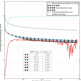
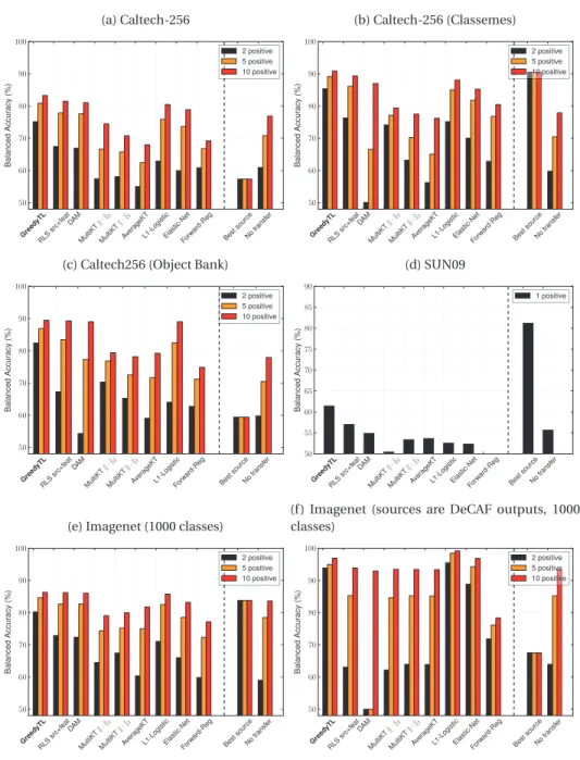
5.1 Empirical tightness of data-dependent and uniform generalization bounds evaluated by training a convolutional neural network. . . 41 6.1 Performance on Caltech-256, subsets of Imagenet (1000 classes) and SUN09 (819 classes).

Averaged class-balanced accuracies in the leave-one-class-out setting. . . 55 6.2 Baselines and number of additional noise dimensions sampled from a standard

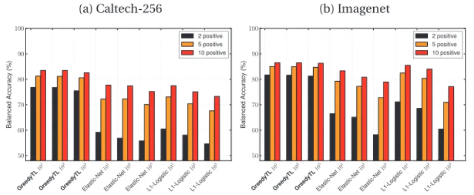
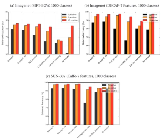
dis-tribution. Averaged class-balanced recognition accuracies in the leave-one-class-out setting. . . 56 6.3 Comparison of the approximated GreedyTL: GreedyTL-59 to GreedyTL with

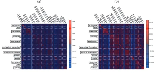
exhaus-tive search and most competiexhaus-tive baselines on three largest datasets considered in our experiments. . . 57 6.4 Semantic transferrability matrix for GreedyTL evaluated on Imagenet (DECAF7 features).

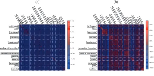
Columns correspond to targets and rows to sources. Stronger color intensity means larger source weight. 6.4a corresponds to learning from 2 positive and 10 negative examples, while 6.4b, with 10 positive. . . 58 6.5 Semantic transferrability matrix for RLS (src+feat) evaluated on Imagenet (DECAF7

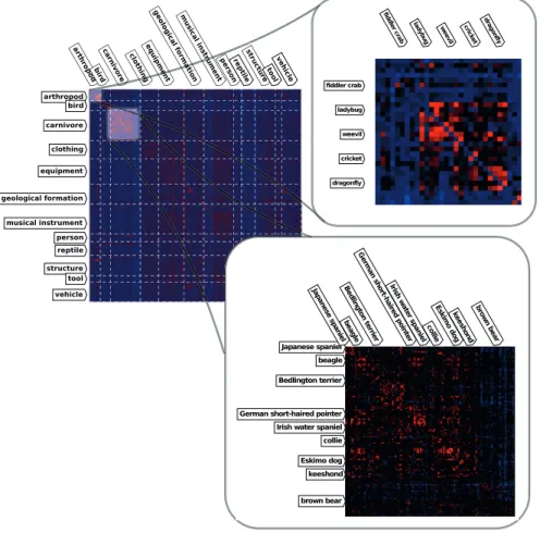
features). . . 59 6.6 GreedyTL evaluated on Imagenet (DECAF7 features): a closer look at some strongly

related sources and targets. . . 59 6.7 Semantic transferrability matrix for the approximated GreedyTL evaluated on Imagenet

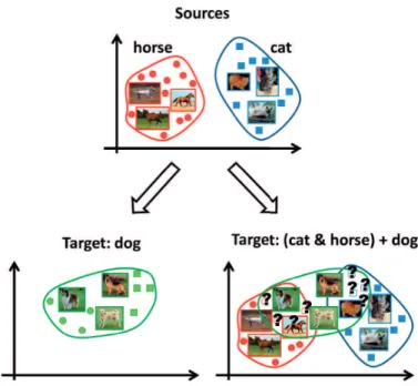
(DECAF7 features). . . 60 7.1 Binary (left) versusK _ÝÑK_`1 transfer learning (right). In both cases, transfer learning

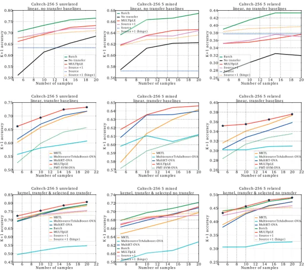
implies that the target class is learned close to where informative sources models are. This is likely to affect negatively performance in theK_ÝÑK_`1 case, where one aims for optimal accuracy on the sources and target classes simultaneously. . . 62 7.2 Experimental results forK_`1_“5, Caltech-256. From left to right, columns report results

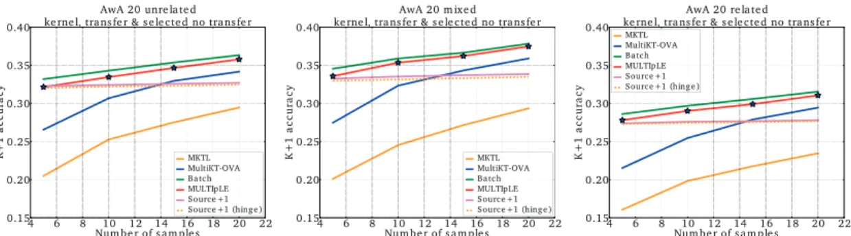
for the unrelated, mixed and related settings. Top row: no transfer baselines, linear case. Middle row: transfer learning baselines, linear case. Bottom row: transfer and competitive no transfer baselines, average of Radial Basis Function (RBF) kernels over all features. Stars represent statistical significance of MULticlass Transfer Incremental LEarning (MULTIpLE) over MultiKT-OVA,p_ă0.05. . . 70 7.3 Results forK_`1_“20, AwA, transfer and competitive no transfer baselines, average

of RBF kernels, all features. Left to right: unrelated, mixed and related settings. Stars represent statistical significance of MULTIpLE over MultiKT-OVA. . . 71

(14)

List of Figures

7.4 Results forK_`1_“20, AwA, unrelated: accuracy over theK sources (left) and over the `1 target (right). . . 73

(15)

List of Tables

6.1 Training time in seconds for transferring to a single target class. Results are averaged over 10 splits. . . 58

(16)

(17)

Acronyms

DA Domain Adaptation

ERM Empirical Risk Minimization

FR Forward Regression

GLS General Learning Setting

HTL Hypothesis Transfer Learning

LOO Leave-One-Out

LSSVM Least-Squares Support Vector Machine

MKL Multiple Kernel Learning

MULTIpLE MULticlass Transfer Incremental LEarning

OVA One-Versus-All

PAC Probably Approximately Correct

PSD Positive Semi-Definite

RBF Radial Basis Function

RKHS Reproducing kernel Hilbert space

RLS Regularized Least Squares

SGD Stochastic Gradient Descent

SVM Support Vector Machine

TL Transfer Learning

UC Uniform Convergence

(18)

Notation

rn_s the sett1, . . . ,nuforn_PN

x,v,u column vectors A,M matrices, e.g.A_{“ r}a1, . . . ,ads }x_}p “´řdi“1|xi|p ¯1 p ,Lp-norm ofx }A_}2 _“sup_}_u_} 2“1}Au}2, spectral norm ofA X Input (instance) space

Y Output (label) space Z Example space,Z_“X_ˆY

D _{Unknown probability distribution over}Z

m Training set size

S “ tziumi“1, a training set drawn iid fromDm H _{Hypothesis space, e.g.}H_“YX _orH _Ď_Rd ℓ Non-negative loss functionH_ˆZ_ÞÑ_R_` }h_}₈ _“sup_x_PXhpxq

}ℓ_}₈ _“sup_w_PH_,_z_PZℓpw,zq

RDphq “E_z_„Drℓph,zqs, risk

RSphq “m´1řim“1ℓph,ziq, empirical risk

RD‹pHq “infhPHRDphq, risk of the best-in-the-class

Tαpxq “maxt´α, mintα,xuu,α-truncation

U_pt1, . . . ,n_uq uniform distribution over 1, . . . ,n

f _“O_p_g_q _D_x₀_,_α_P_R_`_{, such that}_@_x_ą_x₀_,_f_p_x_{q ď}_α_g_p_x_q

f _“O˜_p_g_q _D_k_P_N_{such that}_f _“O_p_logk_p_g_p_x_qq_g_p_x_qq

∇2f_px_q Hessian matrix of a differentiable multi-variate functionf

supp_px_q _{“ t}i_{P r}d_s:xi‰0u

(19)

1 Introduction

The field of machine learning has undergone remarkable advancements in recent years, getting better at addressing rich and highly structured problems, in domains such as computer vision [72, 60], speech recognition [119], machine translation [143], and reinforcement learning [98]. From the algorithmic point of view this is largely a consequence of our increasing capacity to train effective models of high complexity, such as in deep learning. Yet, these qualitative gains usually come at the high price of a tremendous amount of annotated data required to obtain a model of high effectiveness.

This raises a question attractive from both theoretical and practical point of view: how to reduce the sample complexity of an algorithm by exploiting some form of a non-trivial prior knowledge? In the machine learning literature this direction is collectively known astransfer learning. Of course one could argue that it is always possible to simply add more data while increasing the capacity of the model, so why should we bother? There are few counter-arguments to this criticism. First, some problems might come with a small amount of annotated data, thus impeding the use of data-hungry learning, such as deep learning. Indeed, in many applied areas, such as in visual detection, transfer learning is already used in the form of fine-tuning [51] and extraction of feature representations from intermediate layers of neural networks [64]. Second, transfer learning can facilitate training of models with even higher accuracy than those without, at the matching or lower computational cost. Obviously, in such a scenario one can only expect improvements from additional training data. An example is class-incremental transfer learning, where new classes are incorporated into the recognition system, yet every new class could be learned with fewer examples due to some shared similarities with previously observed ones. Finally, it is also conceivable that sample complexity of some learning problems is so high, that practically (w.r.t. available computational resources) we can achieve an acceptable degree of accuracy only through transfer learning. An example of such problem appears in reinforcement learning, where exploration of the vast state-action spaces is intractable, yet due to prior knowledge a successful agent can still be trained. For example, one of the few crucial components in a famous AlphaGo program [126] was based on a neural network pre-trained on a large dataset of human-played games, a form of transfer learning.

In this thesis we focus on theHypothesis Transfer Learning (HTL), a type of efficient transfer learning where information about previously encountered tasks is retained in the form of pre-trained models, or

source hypotheses[76, 77, 80]. This is in contrast to many previous approaches in transfer learning that assume access to the data from another tasks. The critical advantage of HTL is in the computational

(20)

Chapter 1. Introduction

scalability, which from the transfer learning point of view is constrained only by the amount of source hypotheses and by their computational complexity.

1.1 Contributions and Organization

A large part of this thesis concerns the development of an intuitive and practical explanation for established transfer learning algorithms. The first part of this thesis lays out the theoretical foundations of Hypothesis Transfer Learning (HTL) in two learning settings – through Empirical Risk Minimization (ERM) and through stochastic optimization. In Chapter 3 we consider a generalization of a basic yet powerful approach to HTL known as thebiased regularization, related to the Bayesian transfer learning. In particular, we analyze the Regularized Least Squares (RLS) as a hypothesis transfer learning algorithm, and show that its generalization ability critically depends on the quality of the source hypothesis, that is a form of prior knowledge. In this chapter we identify the key quantitative characteristic of relatedness between novel and previous tasks – the expected loss of the source hypothesis on the novel task, and develop generalization bounds explicitating this quantity. This supports theoretically many previous works in the transfer learning literature. In Chapter 4 we further generalize arguments of Chapter 3 and show that the same message holds for ERM approach with respect to any strongly-convex and smooth loss function, with high probability. This chapter also goes beyond generalization analysis and shows that the quality of the source knowledge can accelerate the convergence of the solution to the optimal one within the given set of predictors. Next, in Chapter 5 we consider a different approach to HTL, namely by learning through stochastic optimization. We prove novel data-dependent generalization bounds for Stochastic Gradient Descent (SGD), a popular optimization algorithm used to train deep neural networks and in large-scale learning in general. These bounds allow us to study the generalization ability of HTL through SGD on both convex and non-convex smooth problems. Importantly, this analysis extends the arguments and messages of Chapters 3 and 4 to non-convex problems, such as deep learning. On non-convex problems, in addition to previously established measures of source quality, this analysis identifies the expected curvature at the initialization point as another characteristic that governs success of the transfer learning.

On a more practical side, backed up by theoretical results, the second part of the thesis presents HTL algorithms for binary classification with applications in computer vision. First, in Chapter 6 we present algorithms that address transfer learning with a large number of source hypotheses where the goal is to pick a subset that improves performance on the novel task. Concretely, we propose greedy algorithms for picking such a subset, and in particular a randomized variant with computational complexity independent from the number of source hypotheses. We also show the potential of these algorithms theoretically and experimentally. Generalization bounds corroborate these results, demonstrating that under reasonable assumptions on the source hypotheses these algorithms are able to learn effectively with very limited data. We also investigate HTL beyond the binary classification setting. In Chapter 7 we propose a multiclass classification scenario, where a novel class is learned from few examples by transferring from previously observed classes. This is particularly relevant in lifelong learning, where tasks, e.g. visual categories, faced by the system arrive sequentially. Here, the main algorithmic idea is based upon the biased regularization investigated theoretically in Chapter 3. Again, we demonstrate the transfer learning potential of an algorithm on a visual recognition dataset. Finally, we conclude and present future directions in Chapter 8.

(21)

2 Definitions and Background

The primary goal of this thesis is to provide theoretical foundations for the Hypothesis Transfer Learning (HTL), a successful framework that enables machine learning algorithms to learn from fewer examples on a novel task by leveraging upon auxiliary hypotheses. To accomplish this goal we use tools from statistical learning theory and compare our results to existing theories of learning in a standard non-transfer setting. This chapter introduces necessary definitions, notions, and tools to comprehend the following material. Next, we introduce the learning setting and standard bounds on the performance of learning algorithms. In this thesis we largely follow a constructive theoretical analysis, that is we analyze concrete algorithms and formulations, which is in contrast to the usual uniform convergence argument [141] prevalent in the statistical learning literature. We finalize this chapter by introducing required concepts necessary for this type of analysis.

2.1 Basic notions

Suppose that we have been tasked to design a visual recognition module for a self-driving car that given an image from the camera could tell whether there is a pedestrian in sight. One could try to manually write down the set of all possible visual features characterizing an object in question and try to recognize an object by detecting them. However, due to high natural visual variation this approach would be brittle to unanticipated conditions and most likely would fail. Alternatively one could try to design an algorithm which given a large collection of images under a variety of conditions, with an object and without one, couldlearnthese discriminative characteristics. Thus, the goal of such a

supervised machine learningalgorithm is, given a set of examples, to come up with a hypothesis (a function) able to give correct predictions on yet unseen instances. This is of course only possible by making appropriate assumptions on the environment generating these examples and on the algorithm itself. In this thesis we follow the framework of a statistical learning formalizing such problems, and next we briefly summarize its notions.

In the following we will indicate the space of examples byZ _{and its member by}_z_PZ_{. For instance,} in a supervised settingZ_“X_ˆY_{, such that}X _{is the input and}Y _{is the output space of a learning} problem. In our object recognition case,X _{would stand for the set of all possible images of a certain} size andY would describe all possible annotations, e.g.Y _{“ t}pedestrian, no pedestrian_u. In what follows, without loss of generality we assume that the input spaceX _{is a unit-radius}_L_{2 ball. In addition}

(22)

Chapter 2. Definitions and Background

we introduce a hypothesis classH_{, a set of all admissible hypotheses that the algorithm is allowed to} generate. Thus, formally we define a learning algorithm as a map

A :

8

ď

m“1

Zm_ÞÑH (2.1)

and for brevity we will use the notationAS“ApSq, whereSis a training set. To measure the accuracy

of a learning algorithm, we have a non-negativelossfunctionℓ :H_ˆZ _ÞÑ_R_`, which measures the cost incurred by predicting with some hypothesis fromH _{on an example from}Z_{. We will make use of} the following properties of the loss function as necessary.

Definition 1(L-Lipschitzℓ). A loss functionℓis L-Lipschitz if_}∇ℓ_pw,z_{q} ď}L,_@w_PH and_@z_PZ. Note that this also implies that

|ℓpw,zq ´ℓpv,zq| ďL}w´v}.

Definition 2(β-smoothℓ). A loss function isβ-smooth if_@w,v_PH and_@z_PZ, }∇ℓ_pw,z_{q ´}∇ℓ_pv,z_{q} ď}β_}w_´v_},

which also implies

ℓ_pw,zq ´ℓ_pv,zq ď∇ℓ_pv,zqJpw´vq `β

2}w´v} 2_.

Definition 3(ρ-Lipschitz Hessian ofℓ). A loss function f has aρ-Lipschitz Hessian if_@w,v_PH _and @z_PZ,

}∇2ℓ_pw,z_{q ´}∇2ℓ_pv,z_q}2_ďρ_}w_´v_}.

The last condition is occasionally used in analysis of optimization algorithms and holds wheneverℓ has a bounded third derivative [48].

Intuitively, the prediction should only be possible whenever examples used for training and yet unseen ones share some regularities. The framework of statistical learning captures these regularities by assuming that both training and unseen, or testing data are drawn independently from the same unknown distributionD_{over the example space}Z_{. Then, formally we will denote the training set as}

S_{“ t}ziumi“1 iid

„Dm_{. The distribution}D_{plays a central role in the statistical learning theory, and in some} contexts it is also referred to as thetask. Ultimately we are interested in the performance of a learning algorithm on the testing data sampled from the same task as the training data. This performance is captured by the expected loss or theriskof hypothesish, with respect toD,

RDphq “ E

z„Drℓph,zqs,

and typically we will simply indicateRphq “RDphqwheneverDis clear from the context. Naturally,

(23)

2.2. PAC learning

counterpart measured on the training set, or theempirical riskdefined as

RSphq “ 1 m m ÿ i“1 ℓ_ph,ziq.

2.2 PAC learning

The risk of an algorithm,R_pASq, is a random variable with randomness arising due to the stochastic

origin of the training set (assuming that Ais deterministic). Therefore, risk cannot be computed directly from data, but rather can be estimated using probabilistic bounds. One of the major topics of study in the statistical learning theory is stating such bounds on thegeneralization error, defined as the difference between the risk and the empirical risk of a hypothesis generated by an algorithmA

given a training setS, that is

RDpA_Sq ´R_SpA_Sq. (2.2)

On an intuitive level, if we can describe generalization error in terms of quantities controlled by the algorithm and supplied by the user, such as the training setSand the hypothesis classH_{, then we} can characterize how close the empirical risk will be to the actual performance on unseen data. Thus, whenever generalization error is small or decreases with the size of the training set, we say that the learning algorithmgeneralizes. This is typically sufficient for design of learning algorithms because these bounds point out the ingredients that control generalization. In this thesis we will primarily focus on the generalization bounds.

However, from a theoretical point of view, we sometimes desire to know how optimal the algorithm is, where by optimality we mean the ability of an algorithm to recover the best hypothesis in a given class of functions. To capture this particular notion of optimality1we define the risk of thebest-in-the-class

as

RD‹pHq “ inf

hPHRDphq,

and the optimality of an algorithm is then represented by anestimation error

RDpASq ´RD‹pHq. (2.3)

An estimation error is one of the central notions in statistical learning theory since it formally charac-terizeslearnabilityin a Probably Approximately Correct (PAC) model of learning proposed by Valiant. Here we present its slight extension due to [59].

Definition 4(Agnostic PAC learnability with General Loss Functions). A hypothesis classH is agnostic PAC learnable w.r.t. example spaceZ _{and a loss function}_ℓ _: H _ˆZ_ÞÑ_R_`_{if there exists a function}

mH :p0, 1q2ÞÑNand a learning algorithm A such that for everyǫ,δP p0, 1qand for every distributionD

overZ and every m_ěmHpǫ,δq, with probability at least1´δover a training set Siid„Dm,

RDpASq ´RD‹pHq ďǫ.

(24)

In other words, agnostic PAC learnability formally captures the computational feasibility to address any statistical learning problem by a given class of functions up to certain precision and probability. Another important concept of statistical learning theory, related to PAC learnability, is the uniform convergence.

Definition 5(Uniform Convergence). A hypothesis classH _{has a uniform convergence property w.r.t.}

example spaceZand a loss functionℓ : H_ˆZ_ÞÑ_R_`if there exists a function mUC_H :_p0, 1_q2_ÞÑNsuch that for everyǫ,δ_{P p}0, 1_qand for every distributionD_overZ_{, and every m}_ě_mHpǫ,δq, with probability

at least1_´δover a training set Siid_„Dm,

sup hPH ˇ ˇRDphq ´R_Sphq ˇ ˇ_ďǫ.

Uniform Convergence (UC) goes beyond claims about generalization ability of concrete algorithms and enables analysis of a generalization error for the entire hypothesis classH (that is foranyhypothesis inH_{). An important property of UC is that it is known to imply PAC learnability, see e.g. [123, Corollary} 4.4]. Thus, if one could state a generalization bound for a classH following a UC argument, and then design an algorithm that outputs hypotheses in restriction to that class, then this would imply generalization bound for the algorithm.

Proving the generalization bound for a single fixed hypothesis is straightforward through the standard concentration argument, e.g. using Chernoff bound or a similar one. If we consider more than one hypothesis, forming a finite class, then we could extend this argument by applying union bound, and now our generalization bound would depend on the cardinality of the class. However, since in UC setting we are interested in generalization w.r.t. all hypotheses in a potentially infinitely uncountable class, this approach needs extension towards a more sophisticated way of capturing the capacity of the class.

One popular way to prove UC bounds is through Rademacher complexity analysis, which can be used to prove bounds for both parametric and non-parametric hypothesis classes, e.g. when the class is a subset of a Reproducing kernel Hilbert space (RKHS). This makes its applicability more general than classical combinatorial class capacity measures such as VC-dimension.

Definition 6(Rademacher complexity). LetH _{be a class of functions mapping from}X _toY _and

Siid_„Dm_{. Then Rademacher complexity is defined as}

R_m_pH_{q “} _E S,σ « sup hPH 1 m m ÿ i“1 σihpxiq ﬀ , (2.4) whereσ_{“ r}σ₁, . . . ,σ_m_sJ, withσ_i_„Upt´1,`1uq.

Then one can show [70, 6] the following basic probabilistic UC bound on the generalization error.

Theorem 1. Assume that the loss function is L-Lipschitz and satisfies_}ℓ_}₈_ď1, and that_}h_}₈_{ă 8}. Then with probability at least1´e´2ηover a training set Siid„Dm_{, for every h}_PH _{we have}

R_ph_{q ´}RSphq ď2LRmpHq `

c

η

(25)

2.3. Learning and algorithmic stability

Then stating a generalization bound boils down to actually analyzing the Rademacher complexity of that class. The following lemma states the bound on the Rademacher complexity whenH is anL2 ball.

Lemma 1(Lemma 22 in [6], Theorem 1 in [66]). LetX be a unit L2ball, and let the hypothesis class be

H_τ_{“ t}x_{ÞÑ x}w,x_y :_}w_}2_ďτ_u.

Then Rademacher complexity obeys

R_m_pH_τ_{q ď}_?τ

m .

Theorem 1 in combination with Lemma 1 can be used to state a generalization bound for an algorithm

AS“arg min

}w}2 2ďτ2

RSpwq, (2.6)

which is a special case of theregularized ERM. For example, a particular instance of this algorithm is a well-known Support Vector Machine (SVM).

The bound of Theorem 1 can further be improved to theoptimisticone, which exhibits fastO_p₁_{_m_q_rate of convergence rather than typicalO_p₁_{?_m_q_{subject to some conditions. One example of such bound} presented next guarantees faster generalization subject to the vanishing empirical risk. Practically speaking, whenever a learning algorithm is initialized close to a minimizer of an empirical risk or approached it sufficiently close, the learning switches to the fast rate of convergence.

Theorem 2(Theorem 1 in [129]). Let the non-negative loss function beβ-smooth and let_}ℓ_}₈_ď1. Then with high probability over a training set Siid_„Dm_{, for every h}_PH _{we have}

Rphq ´RSphq “O˜ ¨ ˝τ d βRSphq m ` 1_`βτ m ˛ ‚. (2.7)

2.3 Learning and algorithmic stability

As discussed in the previous section, statistical learning theory usually studies probabilistic bounds on the generalization error that hold for all hypotheses in a given class, that is for any distributionD_with probability at least 1_´δforδ_{P p}0, 1_q,

sup

hPH|

R_ph_{q ´}RSpgq| ďFp1{δ,m, sizepHqq, (2.8)

whereFis a polynomial function of 1_{δ, the number of training examplesm, and some notion of “size” of a class, such as VC-dimension or Rademacher complexity. These bounds are independent from the choice of a learning algorithm.

However, very often we design a concrete learning algorithm and only then analyze its generalization ability. It is also possible that the classH _{is so large that our algorithm explores only a small subset} of it, and therefore UC type of analysis can be too general and would not necessarily lead to good

(26)

estimates. Therefore in many situations it would be sufficient to claim that for any distributionD_with probability at least 1_´δ,

|R_pASq ´RSpASq| ďFp1{δ,m,Aq, (2.9)

whereFis a function polynomial in 1_{δ,m, and some property ofA. Sometimes it is even sufficient to state a deterministic generalization bound

E S “ R_pASq ´RSpASq ‰ ďF_pm,D_,_A_q_. _(2.10)

In contrast to the PAC learnability, this type ofconstructiveanalysis is captured by the General Learning Setting (GLS) due to Vapnik, and the following notion of learnability [124].

Definition 7(Learnability in General Learning Setting). A hypothesis classH _{is learnable w.r.t. example}

spaceZ _{and a loss function}_ℓ _: H_ˆZ _ÞÑ_R_`_{if there exists a learning rule A and a monotonically}

decreasing sequenceǫcons_m , such thatǫcons_m Ñ0as mÑ 8, and @D, E

S„DmrRpASq ´R ‹

DpHqs ďǫconsm . (2.11)

Shalev-Shwartzet al.[124] argued that GLS includes most of statistical learning problems, however for some of them UC actually does not hold. Instead they identified a different well-known property of learning algorithms known as theuniform stability[17] as necessary and sufficient condition for learnability in GLS. Algorithmic stability will be instrumental in constructive analysis of algorithms in this thesis and next we introduce the necessary background.

On an intuitive level, a learning algorithm is said to bestablewhenever a small perturbation in the training set does not affect its outcome too much. Of course, there is a number of ways to formalize the perturbation and the extent of the change in the outcome, and we will discuss some of them below. The most important consequence of a stable algorithm is that itgeneralizesfrom the training set to the unseen data sampled from the same distribution. In other words, the generalization error of an algorithm is controlled by the quantity that captures how stable the algorithm is. So, to observe good performance, or a decreasing risk, we must have a stable algorithmanddecreasing empirical risk (training error), which usually comes by design of the algorithm.

First we consider the following (weak) notion of stability which is known to imply generalization in expectation whenever an algorithm is insensitive to re-sampling of one point in the training set.

Definition 8(On-average stability). Let iiid_„U_prm_sq. Then, a deterministic algorithm A isǫm-on-average

stable if it is true that

E

S,z,irℓpASpiq,ziq ´ℓpAS,ziqs ďǫm. (2.12)

where Siid_„Dm_{and S}piq_{is its copy with i -th example replaced by z}iid_„D_.

Theorem 3(Theorem 13.2 in [123]). Let algorithm A beǫm-on-average stable. Then,

E S “ R_pASq ´RSpASq ‰ ďǫm. (2.13)

(27)

2.3. Learning and algorithmic stability Proof. E S “ RpASq ´RSpASq‰“ E S,z,irℓpAS,zq ´ℓpAS,ziqs (2.14) “ E

S,z,irℓpASpiq,ziq ´ℓpAS,ziqs (Swapzandzisincez,zi

iid „D_.)

ďǫm. (2.15)

As an instructive example consider again a regularized ERM problem (note that this is equivalent to (2.6) wheneverH _Ď_Rd, for some mapping betweenλandτ)

Aλ_S_“arg min wPRd RSpwq `λ}w}2 ( . (2.16)

ThenAλ_Scan be shown to beǫm-on-average stable by appealing to the strong convexity and smoothness

of the objective function.

Theorem 4(Corollary 13.7 in [123]). Assume that the loss function isβ-smooth and non-negative. Then algorithm Aλ_S, assuming thatλ_ě2_mβ, satisfies

ǫm“ 48β mλES “ RSpASq ‰ . (2.17)

This immediately implies a generalization bound in expectation due to Theorem 3. Despite that this bound holds in expectation, other forms of generalization bounds, such as high-probability ones, can be derived from the above [124]. The theorem above can also be used to state a bound on the estimation error and thus prove learnability in GLS.

Corollary 1. Letℓbeβ-smooth and convex w.r.t. hypothesis classH _{and example space}Z _with }ℓ_}₈_ď1. Then settingλ_“

b 150β

9m , we have that for every distributionD,

E

SrRpASqs ´wminPHRpwq ď

c 150β

m . (2.18)

On-average stability discussed above captures sensitivity of an algorithm with respect to a concrete distributionD_{. Therefore we can say that this on-average stability is}_{data-dependent}_{. The following} notion of stability is much more restrictive because it holds uniformly for the choice of any data and characterizes stability as a property of a learning algorithm.

Definition 9(Uniform stability). A deterministic algorithm A isǫuni_m -uniformly stable if for all datasets S,Spiq_PZm_{such that S and S}piq_{differ in the i -th example, we have}

sup

zPZ,iPrmst

ℓ_pA_Spiq,zq ´ℓpAS,zqu ďǫunim . (2.19)

Although more restrictive than on-average stability, uniform stability is usually easier to work with, because one can completely rely on a geometrical argument and tools from optimization leaving out

(28)

probabilistic details. The following theorem implies that uniform stability implies generalization with high probability.

Theorem 5(Theorem 12 in [17]). Assume that the loss function satisfies}ℓ_}₈_ďM . Then with proba-bility at least1_´e´2ηover a training set Siid_„Dm_{, for algorithm A we have that}

R_pASq ´RSpASq ď2ǫunim ` p2mǫunim `Mq

c

η

m . (2.20)

Naturallyǫmďǫunim , and by Theorem 4 we get that

ǫuni_m _ď48Mβ

(29)

Part I

(30)

(31)

3 Hypothesis Transfer Learning through

Regularized Least Squares

The material of this chapter is based on the publication:

I. Kuzborskij and F. Orabona. Stability and Hypothesis Transfer Learning.

InProceedings of the International Conference on Machine Learning (ICML), 2013.

The doctoral candidate formalized the problem, proved the results, and wrote most of the publica-tion.

3.1 Overview

The standard assumption made during design of supervised machine learning algorithms is to have models trained and tested on samples drawn from the same probability distribution, ordomains. However, this assumption is often violated in practical applications.

A more general setting is the one in which the marginal distributions associated with training and testing domains are different but related. This is the problem of Domain Adaptation (DA), where a successful scheme typically utilizes large unlabeled samples from both domains to adapt a source hypothesis to the target domain. Previous work has addressed in detail the theory of DA and proposed algorithms that critically depend on optimal weighting parameters given by the theoretical analysis [8, 9, 93, 27]. However, in practice, the learner needs access to sufficient unlabeled samples from both domains to estimate these parameters. Even if unlabeled data are abundant, the estimation of these parameters can be computationally prohibitive in some scenarios. A hypothetical example is a large number of domains involved or, for instance, when one acquires new domains incrementally. Here, keeping unlabeled data from all the domains and re-estimating parameters is a necessity.

To overcome this practical limitation, a new framework has been analyzed by a number of works [45, 145, 103, 94, 136, 78]. In this framework, that we will call Hypothesis Transfer Learning (HTL), unlike DA, onlysource hypothesesare retained from the source domain, but not the source data. The attractive quality of HTL is the fact that it assumes no explicit access to the source domain, nor any knowledge

(32)

Chapter 3. Hypothesis Transfer Learning through Regularized Least Squares

about the relatedness of the source and target distributions. Although, this setting has been explored empirically with success, a formal theory of HTL is mostly missing. Hence it is unclear how to recover optimal transfer parameters and what properties of the source hypothesis affect generalization. In this chapter, we take a step towards a theory of HTL. In particular, we analyze the generalization ability of an HTL algorithm stemming from the Regularized Least Squares (RLS) with biased regular-ization. We assume access to a given number of source hypotheses and asmallset of training samples from the target domain. Rather than relying on oracle inequalities for tuning the optimal parameters, we use the Leave-One-Out (LOO) risk. The LOO risk is known to have low bias compared to empirical risk or cross-validation [43], thus making it preferable in a small sample regime.

In this chapter we will show that the generalization error of the considered HTL algorithm decreases with the increasing quality of the source hypothesis over the target domain. We do so by employing the notion ofhypothesis stability[17], a form of on-average stability, and upper bounding the second-order moment of the difference between the expected risk and the LOO risk. In addition, we propose a hypothetical algorithm that can avoid negative transfer in the case of unrelated domains, while in worst case scenario recovering the generalization guarantees of RLS. Finally, from the stability theory point of view, this chapter also touches upon a question raised by [43]:“Is there a way to incorporate prior knowledge via stability?”, thus exposing a connection between stability and the Hypothesis Transfer Learning.

The rest of the chapter is organized as follows. We formally state the HTL problem in Section 3.2 and introduce analyzed algorithms in Section 3.4. The main result comes in Section 3.5, particularly in Theorem 7, with implications discussed in Section 3.5.1. The proof of the main result can be found in Appendix A, while related work on DA and HTL is covered in Section 3.3. Finally we draw some conclusions and discuss future work in Section 3.6.

3.2 Hypothesis Transfer Learning Problem

First we formally describe the transfer learning problem we consider in this chapter. Assume that in addition to the training setSwe also receive asourcehypothesishsrc_PHsrc_ĎYX. Then, the aim of an HTL algorithm is to use the source hypothesishsrcto improve the performance compared to the supervised learning algorithm that has access only toS. More formally, we define the HTL algorithm as follows

Definition 10(HTL algorithm). An HTL algorithm is a map

Ahtl: ˜ ₈ ď m“1 Zm ¸ ˆHsrc_ÞÑH . (3.1)

The following definition captures the goal of an HTL algorithmAhtlmore formally.

Definition 11(Usefulness and Collaboration). We say that hypothesis hsrc_PHsrc_is_useful_{[76] for A}htl

with respect to distributionDand training set size m, if

E S “ RDpAhtlpS,hsrcqq ‰ ăE S “ RDpAhtlpS,0qq ‰ . (3.2)

(33)

3.3. Related Work

In addition, we will say that hsrc_PHsrc_{and a distribution}D_collaborate_{[11] for A}htl_{, w.r.t. training set}

size m, if E S “ RDpAhtlpS,hsrcqq ‰ ămin ! RDpAhtlp∅,hsrcqq,E S “ RDpAhtlpS,0qq ‰) .

The first notion (usefulness) is satisfied whenever algorithmAhtl_S can achieve lower risk by using the source hypothesis. The second one (collaboration) [11] is satisfied whenever simultaneous access tohsrcandSimproves the performance compared to when they are used separately. The failure to satisfy any of these two conditions is usually called thenegative transfer. Thus, we are only interested in the observable improvement of the generalization error on the target domain. From now on we will indicateAhtl_S _“Ahtl_pS,hsrc_qas for the most part of this chapter we will consider the use of a single source hypothesishsrc.

3.3 Related Work

We start by introducing related work from Domain Adaptation (DA), closely related to the HTL problem. Most DA algorithms assume access to the labeledmsrc-sized training set sampled from the source domainDsrc_{, a sample of}_munlab_{unlabeled examples from both domains (marginal distributions), and} occasionally anm-sized training set sampled from the target domain. Typically it is assumed that

m_!msrc,m_!munlab.

A milestone work on theoretical analysis of DA is due to Ben-Davidet al.[8], where they considered unsupervised setting. The main result of [8] is a UC-type bound on the difference between risks on the target and source domains. This bound is controlled by two critical terms: the “divergence” term and the minimal-joint-error, defined with respect to some hypothesis class. The divergence term quantifies how different distributions (domains) are, while the second term quantitatively captures the existence of a hypothesis with low error on both domains. The theoretical nature of the divergence term was later futher investigated by [9]: the additive divergence term is inevitable unless an algorithm has access to labeled training data from the target domain. A similar theoretical setting was also studied by [93]. Once again, an additive divergence term appears in the bounds. Although related, the HTL problem is not covered by the DA theory because it depends on the properties of the learning algorithm that generates the source hypothesis. More importantly, the source domain is inaccessible. These facts render the mentioned DA bounds unapplicable for analysis of the Hypothesis Transfer Learning. HTL has been also investigated from Bayesian perspective. Li and Bilmes [86] proposed a PAC-Bayes-type of analysis and derived bounds capturing the relationship between domains by an additive KL-divergence term. They showed that for logistic regression, the divergence term is upper bounded by_}h_´hsrc_}2, motivating the biased regularization term in logistic regression. Indeed, Bayesian linear regression withhsrc-mean Gaussian prior overhleads to exact recovery of_}h_´hsrc_}2in optimization problem [13]. Results of [86] hint that generative methods like the one in [45] could also be related to biased regularization.

The majority of algorithmic works on DA focus on recovery of transformations that approximately minimize the divergence term. Many of these works have further investigated the use of more powerful transformations by lifting computations into the RKHS [55, 104, 4, 148], thus paving the way for DA

(34)

in non-linear learning problems. The found transformations are then used to map the hypothesis generated on the source domain in hope that it would perform well on the target one. At the same time the transformation is typically found on the basis of large unlabeled samples drawn from marginal distrubutions. Unfortunately many of these works are known to scale badly inmunlabandmsrc, therefore evaluations are rarely done beyond the proof-of-concept benchmarks. At the same time HTL is only limited by computational complexity of the source hypothesis.

Motivated from this point of view, a number of empirical attempts have tried to justify HTL. An SVM-like algorithm with regularizer_}h_´hsrc_}2was proposed by [145] for video concept detection. Orabonaet al.[103] suggested a parametrized variant,_}h_´βhsrc_}2-regularized Least-Squares Support Vector Machine (LSSVM), then extended to weight and combine multiple source hypotheses in [136]. Leveraging on this idea, an HTL multiclass formulation explored a class-incremental transfer set-ting [78]. While some of these methods demonstrated impressive practical potential, their theoretical nature remains unclear.

3.4 Hypothesis Transfer Learning through Regularized Least Squares

First we introduce additional definitions used only throughout this chapter. Without loss of generality, in the following we will assume thatY_,Y1_{“ r´}_B_;_B_s_{, where}_B _P_R_and_}_x_{} ď}_1, _x _PX _“_Rd_{. In} addition to the training setSwe also defined the LOO training set asSzi_{“ tp}x1,y1q,pxi´1,yi´1q, . . . ,

pxi`1,yi`1q,pxm,ymquand hypothesishSziis produced by an algorithmAgiven training setSzi. Then,

we also define theLOO riskas

Rloo_pA,S_{q “} 1 m m ÿ i“1 ℓ_pA_Szi,pxi,yiqq.

We will consider linear algorithms, extended to non-linear ones through the use of kernels. Hence hypothesish_px_qwill be expressed as the inner product of a vectorw, learned from the training data, and the samplex.

We assume, that only the target training setSand source hypothesishsrcare given, so that the source training set is not required. The main objective of this analysis is to identify the effect ofhsrcon the generalization properties ofAhtl. For this reason, we would like to bound the expected risk ofAhtl

with terms depending on the characteristics ofhsrc. In particular, we expect that a smaller riskR_phsrc_q

should improve the generalization ofAhtl, compared to the case whenhsrc_”0.

As said above, we proceed by specializingAhtlto a particular class of algorithms, the RLS with biased regularization. This will allow us to arrive at a generalization bound where all the relevant quantities are computable in a closed form.

(35)

3.4. Hypothesis Transfer Learning through Regularized Least Squares

3.4.1 Biased Regularized Least Squares

The RLS algorithm consists in solving the following optimization problem

min wPRd # 1 m m ÿ i“1 pwJxi´yiq2`λ}w}2 + . (3.3)

The interest of RLS lies in its strong theoretical guarantees and in the fact that the solution can be expressed in a closed form [116]. As a useful consequence, its LOO prediction function is expressed in closed form as well, allowing a very efficient model selection [21]. It is also possible to arrive at (3.3) from a Bayesian perspective by putting a0-mean Gaussian prior over the parameters of a linear regression model [13]. Note that the same formulation can be used for both classification and regression problems [116, 132].

Assuming that the source hypothesishsrc_px_qis expressed asxJw0, andw0belongs to the same space ofw, [103] proposed the use of a biased regularization to solve hypothesis transfer learning problems efficiently. More formally they defined the following algorithm.

Algorithm 1. The Hypothesis Transfer Learning Algorithm based on Regularized Least Squares generates a hypothesis Ahtl_S ´bias_px_{q “}xJwS, where

wS“arg min wPRd # 1 m m ÿ i“1 pwJxi´yiq2`λ}w´w0}2 + . (3.4)

Analogously, one can see the formulation of Algorithm 1 as a Bayesian linear regression withw0-mean Gaussian prior distribution. The solution of Algorithm 1 can be expressed in closed form, in fact from the first order optimality condition we get

wS“ arg min wPRd !₁ m}X J_w_´_y_}2 `λ_}w_´w_0}2 ) ñX_pXJwS´yq `mλpwS´w0q “0 (3.5) ñX_pXJwˆS`XJw0´yq `mλwˆS“0 ñ pX XJ_`mλI_qwˆS“X y´X XJw0 ñwˆS“ pX XJ`mλIq´1Xpy´XJw0q ñwˆS“XpXJX`mλIq´1py´XJw0q

where in (3.5) we used ˆwS“wS´w0and in the last step we used the identitypX XJ`mλIq´1X “

X_pXJX_`mλI_q´1to express the solution in dual variables. So, the solution to the problem is given by

wS“XpXJX`mλIq´1py´XJw0q `w0, due the definition ofwS.

Using the fact that the LOO risk of Algorithm 1 can be written in closed form, [103] proposed to weight the source hypothesisw0by a scalarβ, optimized in order to minimize the LOO risk.

In the following we show how to generalize this approach to the generic source hypotheseshsrcand how to obtain a generalization guarantee for it.

(36)

3.5 Analysis by Hypothesis Stability

We now propose a more general version of Algorithm 1.

Algorithm 2. RLS transfer algorithm by altering training set as_tpxi,yi´hsrcpxiqq: 1ďiďmuproduces

a hypothesis Ahtl_S _px_{q “}TCpxJwSq `hsrcpxq, where wS:“arg min wPRd # 1 m m ÿ i“1 pwJxi´yi`hsrcpxiqq2`λ}w}2 + ,

and the truncation function TCpyqis defined as TCpyq “mintmaxty,´Cu,Cu.

Ifhsrc_px_qis equal toxJw0, wherew0belongs to the same space aswS, andC“ 8, Algorithms 1 and 2

are completely equivalent, because they have exactly the same solution. However, Algorithm 2 is more general because it allowshsrcto belong to a another hypothesis class. Hence it captures the notion of biased regularization, and generalizes it to any type of source hypothesishsrc. This algorithm also captures and generalizes many of the ideas present in the previous works on HTL [45, 145, 103, 94, 136]. Still the use of a specific loss, the square loss, will allow us to have an efficient computation as well. Also, this formulation allows us to truncate the prediction within the rangerĆ;Cs, which improves the theoretical guarantees and the practical performance. In fact it is easy to see that ifC_ěB_`}hsrc_}₈, thenpTCpxJwSq `hsrcpxq ýq2ď pxJwS`hsrcpxq ýq2.

Our goal is to upper bound the expected risk of Algorithm 2, keeping in mind the effect ofhsrc. To this end, we propose to employ the stability framework of [17]. Our choice is motivated by the fact that bounds arising from the stability analysis are free from complexity measures. Hence, the generalization bound of interest will be composed mostly from computable quantities, thus making it more practical, e.g. for finding the optimal transfer parameters.

In particular, we can upper bound the moments of the random variableR_pASq ´RloopA,Sqwith a

quantity that captures the stability of the learning algorithm. The second order moment can then be used to obtain polynomial bounds, through Chebyshev’s inequality [17].

There are various definitions of algorithmic stability [17], but the one we will use is the hypothesis stability.

Definition 12(Hypothesis Stability [17]). An algorithm A has a hypothesis stabilityγwith respect to the loss functionℓif for all i_{P t}1, . . . ,m_uthe following holds

E

S,px,yqr|ℓpAS,px,yqq ´ℓpASzi,px,yqq|s ďγ.

We will use a slight variation of the polynomial bound of [17]. The reason is that Theorem 11 in [17] has the termM₂2, that is not affected byR_phsrc_q. Instead, we exchangeM₂2 for the termESrℓphSzi,ziqs.