White Rose Research Online URL for this paper:
http://eprints.whiterose.ac.uk/130258/
Version: Published Version
Article:
Motazedi, N. and Beck, S. orcid.org/0000-0003-2673-4179 (2017) Leak detection using
cepstrum of cross-correlation of transient pressure wave signals. Proceedings of the
Institution of Mechanical Engineers, Part C: Journal of Mechanical Engineering Science .
ISSN 0954-4062
https://doi.org/10.1177/0954406217722805
© IMechE 2017. This article is distributed under the terms of the Creative Commons
Attribution 4.0 License (http://www.creativecommons.org/licenses/by/4.0/) which permits
any use, reproduction and distribution of the work without further permission provided the
original work is attributed as specified on the SAGE and Open Access pages
(https://us.sagepub.com/en-us/nam/open-access-at-sage).
eprints@whiterose.ac.uk https://eprints.whiterose.ac.uk/
Reuse
This article is distributed under the terms of the Creative Commons Attribution (CC BY) licence. This licence allows you to distribute, remix, tweak, and build upon the work, even commercially, as long as you credit the authors for the original work. More information and the full terms of the licence here:
https://creativecommons.org/licenses/
Takedown
If you consider content in White Rose Research Online to be in breach of UK law, please notify us by
Leak detection using cepstrum of
cross-correlation of transient
pressure wave signals
Niloufar Motazedi and Stephen Beck
Abstract
A new leak detection method is proposed here which is based on the cepstrum of the cross-correlation of the pressure signals from two transducers. Computational simulations of leaks with different properties, size, position and shape, in a straight pipe and a T-Junction network were studied. The proposed method was successful in estimating leakages and the pipeline features with a high precision. For the results with a straight pipe, this method is considerably more accurate than using the cross-correlation leak detection method or the cepstrum method alone. However, the results obtained by cepstrum and cepstrum of cross-correlation for the T-Junction case were quite accurate, while cepstrum alone showed a slightly better precision.
Keywords
Transient leak detection, cepstrum analysis, cross-correlation method, unsteady flow, computational fluid dynamics Date received: 19 January 2017; accepted: 4 July 2017
Introduction
Leaks within pipeline systems are mainly caused by excessive pressures, material defects, ageing, external events and vibrations. Successful development of leak detection methods have been achieved in sectors where the final product value is much higher than the leak detection costs, such as the chemical, gas and oil industries. However, the massive growth in population rate, environmental hazards, public health and financial losses over water pipeline leakage has raised many concerns for the governments, pipe-line owners and water suppliers. Therefore, develop-ing an effective and affordable leak detection method has become a major priority.
Transient leak detection methods have the potential to be a robust, functional and low cost leak detection method in the future.1In these meth-ods, a transient pressure wave is introduced to a system by a sudden change in the static pressure at the inlet (hydraulic shock/water hammer effect); this wave is mostly apositive pressurewave and it travels away from the place where it was caused.2–4When a
positive pressure wave encounters a pipeline feature, such as a junction, a pump, or a leak, a lower ampli-tude pressure wave reflects back towards where it came from.5The reflected wave is known as anegative pressureor rarefactionwave. Capturing the signal of these pressure waves at suitable locations in the
system can provide very useful information about the system status.
This paper investigates the application of the cep-strum of the cross-correlation signal of static pressure for leak detection purposes. By applying a transient pressure wave to a straight pipeline (both 2D and 3D) and a T-Junction (2D), various leak types were inves-tigated. Furthermore, the generated results are com-pared with the cross-correlation and cepstrum leak detection methods.6–8
There are various types of transient leak detection methods, using different signal processing approaches notably by the Sheffield9 and Perugia groups.10–12 Leak detection based on the cross-correlation method has been used for leak detection purposes in several studies. Beck et al.6,7applied the cross-correla-tion and its derivatives to identify pipeline features and a leaks, using one sensor. The experimental and numerical results were in an acceptable range. Hanson et al.13compared the cepstrum analysis and the cross-correlation method on the noise and vibration signals
Department of Mechanical Engineering, University of Sheffield, Sheffield, UK
Corresponding author:
Stephen Beck, The University of Sheffield, Multidisciplinary Engineering Education, The Diamond, Floor 1, Room C.10c, 32 Leavygreave Road, Sheffield S3 7RD, UK.
Email: s.beck@sheffield.ac.uk
Proc IMechE Part C:
J Mechanical Engineering Science 0(0) 1–13
!IMechE 2017 Reprints and permissions:
sagepub.co.uk/journalsPermissions.nav DOI: 10.1177/0954406217722805 journals.sagepub.com/home/pic
generated by a leak. In this numerical study, a leak was modelled as white noise. Both methods per-formed correctly in this idealised simulation with uncorrelated noise. However, acoustic method appli-cations are limited by distance of the sources of noise to the sensors, and pipe material. In a numerical study, Motazedi and Beck14 have used cross-correla-tion and its derivatives to identify different type of leakage in a straight pipe, using two sensors. In all cases, the leak was detected with less than a 2.5% error.
The application of the cepstrum analysis specific-ally for leak identification has been considered in a few published studies. Le et al.15 have compared the performance of a cepstrum analysis using a linear pre-diction coding16within a multilayer perception neural network. Two pressure transducers at the outlet were installed to measure the transient wave. In conclusion, the results generated by using the cepstrum technique were claimed to be more accurate (95%) than the other method.
In an experimental approach, Taghvaei et al.17 investigated a T-Junction pipeline system with differ-ent leak sizes (diameter of 2 and 4 mm) at a single location. The pressure transient was created by using a solenoid valve and the pressure signal was measured near the system inlet. The output data were filtered by using the Orthogonal Wavelet Transform (OWT) and the location of the leak was predicted by the cepstrum method. For the case where the system has no leaks in the pipeline, the locations of the inlet and both outlets were estimated with a maximum error of 7.4%. The position of 2 and 4 mm leaks are detected with an error of 1.07% and 1.57%, respectively. It was also noted that the cep-strum amplitude had increased when enlarging the leak diameter. A computational fluid dynamic (CFD) study has been done based on this experiment and a leak was located with an error of 0.5%. Furthermore, a cepstrum analysis was applied to tran-sient pressure signals in a 90 m pipe in an oval loop shape with six loops. Different leak sizes at two fixed locations, 35 and 72.5 mm from the system inlet, were created by using small ball valve. The errors for iden-tifying the location of leaks, with the flow rates of 0.20, 0.25, 0.30 and 0.40 L/s, were claimed to be less than 0.7%.
Ghazali et al.9 studied the analysis of a transient pressure wave in a live water distribution system using a variety of instantaneous frequency (IF) techniques. Methods such as, Hilbert Transform (HT), Normalised Hilbert Transform (NHT), Direct Quadrature (DQ), Teager Energy Operator (TEO) and cepstrum were applied to the system. Results showed much more accurate estimations were acquired by using NHT and DQ, while TEO showed a moderate performance, interestingly and highly relevant to this present work, the cepstrum result was the least accurate method.
In an experimental investigation,18 the effect of changing the size and shape of small leaks were inves-tigated, using a pressure-time history at one section of the pipe. The sensitivity of the pressure signal on the inlet and outlet boundary conditions were also con-sidered. Small leaks with circular, triangle, rectangu-lar and square leaks were tested. The results confirmed a dependence between the measured pres-sure signal and the shape and size of small leaks.
Methodology
CFD simulations were conducted to model various leak properties in two different computational domains. A transient pressure wave was created by introducing a hydraulic shock at the inlet of each system. Two sensors were used to monitor the static pressure during the transient event. The speed of the pressure wave was calculated using the travel time of the pressure wave between sensors.
As the pipeline components have a fixed position, the introduced transient pressure wave creates reflec-tions with constant time lags. All the signals have a defined start point at time zero (the transient event) as well as delays corresponding to the echo delay time. Therefore, the cross-correlation function has peaks corresponding to the echo delay times, giving delta functions in the cepstrum, and also delays times between the different signals. Thus, the transient pres-sure wave travels through the system for a consider-able amount of time, the time lags (peaks) of the cross-correlation profile will be repeated with con-stant frequencies/time.
Cross-correlation
The similarities between two signals, p and q, were determined using the cross-correlation technique.19 Equation (1) shows the cross-correlation signal (r) between the inlet (p) and outletqstatic pressure out-puts during the simulation (n and k represent the respective data point (index) number).
rðkÞ ¼X
þ1 1
pðnÞqðnþkÞ ð1Þ
Complex cepstrum
Generally, there are three types of cepstrum analysis: the power cepstrum, complex cepstrum and real cep-strum. The power cepstrum can be used for echo iden-tifications and it is not valid for wavelet recovery, as the phase information is lost.20–23 Real cepstrum is defined as inverse Fourier transform (IFT) of the log amplitude spectrum. This method is mostly used where the phase measurement is not required. Complex cepstrum, which is used in this research, is mostly applied to well-behave signals such as
impulse responses. The phase in the complex cepstrum must be unwrapped for a continuous function of frequencies. The complex cepstrum of the cross-correlation signal r(k) and inlet pressure p(k) are derived to identify local singularities and harmonics within the signal’s history. The complex cepstrum method is defined as the IFT of the logarithm of the Fourier transform of the signal; therefore, it is revers-ible to the time domain.20,24 Equation (2) shows the Fourier transform of the input signalQ(x), whereFis
the Fourier transform,A(x) is the amplitude,(x) is
the phase andj¼ ffiffiffiffiffiffiffi
1 p
.
Qð!Þ ¼FfrðkÞg ¼ jAð!Þjejð!Þ ð2Þ
The logarithmic form of Q(x) is given in
equation (3).
logQð!Þ ¼logjAð!Þj þjð!Þ ð3Þ The definition for the complex cestrum is shown in equation (4), whereF1 is the IFT.25
CA¼F1flogQð!Þg ¼F1ðlogjAð!ÞjÞ þjð!Þ
ð4Þ The autocorrelation function can be defined as the IFT of the power spectrum, whereas the cepstrum is the IFT of the logarithm of the estimated spectrum of a signal. The cepstrum method is not sensitive to the
(a)
(b)
Figure 1. Computational domains descriptions: (a) T-Junction, (b) straight pipe. x: distance of the leak from the inlet, d: leak diameter.
colour of the spectrum and creates delta functions to echoes. However, the autocorrelation method only gives a delta function, where the spectrum is in white (either white noise or impulse). It should be noted that when the length of the autocorrelation function is inversely proportional to the 3-dB band-width of the narrowest resonance peak, where the signal is coloured within a system with resonances. As the results show, dispersion of the signal does not manifestly affect the results.
Numerical simulations
The commercial ANSYS FLUENT (CFD) code was used to simulate different pipeline systems. In this study, two general types of computational domains have been assessed: a T-Junction (Figure 1(a)) and
a straight pipe (Figure 1(b)). Several leak properties have been investigated by changing the leak diameter (d) and the distance of the leak from the inlet (x) in a straight pipe. Table 1 summarises the properties of each case and its corresponding computational domain.
Modelling considerations
In all the simulations, a similar solution method has been applied. Liquid compressible water (using the Tait formulation26) at a temperature of 300 K was used as the working fluid. The density of water,
q, was set to 998.2 (kg=m3), and the water bulk
modu-lus KW was 2.16 GPa. The theoretical speed of the
pressure wave was equal to 1471.7 m/s, using the standard equation, ffiffiffiffiffiffiffiffiffiffiffiffi
KW=
p .
To introduce the transient pressure wave, the inlet pressure from the steady state condition of 15,000 Pa (Re¼83,177) was dropped to 2500 Pa (Re¼33,957) after 22.2ms.
The boundary condition for the outlets and leaks were set to atmospheric pressure. No-slip boundary conditions were assigned to the walls. It will be noted that both two- and three-dimensional models were conducted. The 2D models were in effect of an infinite flow channel with an slit for the leak. The 3D models were more accurate, with the leak modelled as a hole in the pipe, but these were computationally far more expensive to run.
Solution methods
The standard k-2scheme was applied for turbulence modelling.27The turbulent length scale was set to the internal diameter of the pipe and the turbulent inten-sity at the inlet was set to 10%. The SIMPLE scheme was used for pressure-velocity coupling. The second-order upwind scheme was used as the discretisation method for the momentum, turbulent kinetic energy and dissipation rates. In the unsteady simulations,
Table 1. Case studies specifications.
Type Name x (m) d (m) Leak geometry 2D T-Junction TCP 6 0.005 N/A Straight pipe 2D65 6 0.005 2D62 6 0.002 2D61 6 0.001 2D45 4 0.004 2D55 5 0.005 Type Name x (m) Area (mm2) Leak geometry 3D Straight pipe 3D10C 10 0.19 Circular 3D6C 6 Circular 3DLE 6 Longitudinal ellipse 3DTE 6 Transverse ellipse 3D5C 5 Circular 3D4C 4 Circular t(s)x10-3 0 5 P ( Pa ) 0 2000 4000 6000 8000 10000 12000 (b) t(s)x10-3 0 2 4 P ( Pa ) -3000 -2000 -1000 0 1000 (c) t(s)x10-3 -2 0 2 4 P ( Pa ) 4000 6000 8000 10000 12000 14000 16000 (a)
the transient formulations (pressure, momentum, tur-bulent kinetic energy and turtur-bulent dissipation rate) were set to second-order.
After comparing a wide range of structured quad-rilateral mesh densities, meshes with 6000 and 180,000 nodes for 2D and 3D straight pipelines, respectively, were selected, whilst the mesh density for the T-Junction case was about 7000 nodes. In these unsteady cases, the time step of 105s was deemed
to be acceptable to capture the key flow features.
Results and discussion
Figure 2 shows the variation of the introduced transi-ent wave at differtransi-ent positions of the straight pipe com-putational domain. The original defined inlet pressure profile is shown in Figure 2(a). Figure 2(b) highlights the measured profile at the inlet sensor, whilst, Figure 2(c) shows the captured transient wave just before a leakage. In Figure 2(c), the introduced
transient wave is shown as a sudden pressure drop after about 4 ms, and then after a short delay, the pres-sure can be seen to increase, due to the arrival of the reflectednegative pressurewave from the leak. As the introduced transient wave is the same for all the simu-lations, one would expect the same type of response for all the T-Junction simulations.
The introduced transient pressure wave and its reflections were measured 0.01 m after the inlet and before the outlet. Consequently, the cepstrum, the cross-correlation and the cepstrum of cross-correla-tion signal analysis methods were applied to a variety of cases for both straight pipe and T-Junction geome-tries and hence computational domains. The results are individually discussed and compared later.
Straight pipe
Different leak properties (size, position and geometry) were numerically simulated in a straight pipeline,
x(m) 2 3 4 5 6 7 8 9 10 F − 1{ lo g P ( ω ) } -0.03 -0.02 -0.01 0 (a) 2D61 2D62 2D65 x(m) 2 3 4 5 6 7 8 9 10 F − 1{ lo g P ( ω ) } -0.06 -0.04 -0.02 0 0.02 (b) 2D45 2D55 2D65 x(m) 2 3 4 5 6 7 8 9 10 F − 1{ lo g P ( ω ) } -0.08 -0.06 -0.04 -0.02 0 0.02 0.04 (c) 3D4C 3D5C 3D6C x(m) 2 3 4 5 6 7 8 9 10 F − 1{ lo g P ( ω ) } -0.08 -0.06 -0.04 -0.02 0 0.02 (e) 3D6C 3DLE 3DTE x(m) 2 4 6 8 10 12 14 16 18 20 F − 1{ lo g P ( ω ) } -0.04 -0.02 0 0.02 (d) 3D10C
Figure 3. The cepstrum of the inlet pressure signals for different leak geometries: (a) 2D models with different leak sizes, (b) 2D models with leak at different positions in the pipe (4, 5 and 6 m), (c) 3D models with leak at different positions of the pipe (4, 5 and 6 m), (d) 3D models with leak placed at different positions of the pipe (10 m) and (e) 3D leak with various geometries (circular, longitudinal ellipse and transverse ellipse).
x(m) 0 5 10 15 20 25 30 35 40 r ( t ) ×108 -4 -2 0 2 (a) 2D61 2D62 2D65 x(m) 0 5 10 15 20 25 30 35 40 r ( t ) ×108 -4 -2 0 2 (b) 2D45 2D55 2D65 x(m) 0 5 10 15 20 25 30 35 40 r ( t ) ×108 -4 -2 0 2 (c) 3D4C 3D5C 3D6C x(m) 0 5 10 15 20 25 30 35 40 r ( t ) ×108 -6 -4 -2 0 2 (e) 3D6C 3DLE 3DTE x(m) -10 -5 0 5 10 15 20 25 30 r ( t ) ×107 -6 -4 -2 0 (d) 3D10C
Figure 4. The cross-correlation results for different leak geometries: (a) 2D cases with different leak sizes, (b) 2D cases with a leak placed at different positions in the pipe (4, 5 and 6 m), (c) 3D cases leak placed at different positions of the pipe (4, 5 and 6 m), (d) 3D cases, leak placed at different positions in the pipe (10 m) and (e) 3D leak with various geometries (circular, longitudinal ellipse and transverse ellipse).
Figure 5. Use of the proposed method for the 3D4C case: (a) Cross-correlation signal and (b) cepstrum of cross-correlation results.
both 2D and 3D. The pressure signal 0.01 m after inlet and before the pipe outlet was monitored. The speed of sound inside the pipeline was determined by the time that the introduced transient pressure wave requires to reach the outlet; which gave a celerity of 1471.7 m/s (the signal time is converted to distance using this value). The measured celerity is equal to the theoretical value, which is given in the ‘Modelling considerations’ section of the paper.
The cepstrum method. The cepstrum of the inlet pres-sure signal on its own is used to estimate the leak location in the straight pipeline cases (Figure 3).
A very sharp peak can be observed at the distance from each of the leaks to the inlet sensor. Figure 3(a) shows the results for 2D cases with differ-ent leak size at 6 m from the inlet, the leak is predicted with a slight variation of 1% in all cases. The cep-strum results for different leak positions in both 2D and 3D simulations are shown in Figure 3(b) to (d), the errors in predicting the leak location was consid-erably lower for the 3D cases. Furthermore, changing the leak geometry has not affected the results, the lon-gitudinal and transverse ellipse and the circular leaks were detected with exactly the same precision (1%). Comparing the results with Brunone and Ferrante,18
x(m) 2 3 4 5 6 7 8 9 10 F − 1{ lo g R ( ω ) } -0.05 0 0.05 (a) 2D61 2D62 2D65 x(m) 2 3 4 5 6 7 8 9 10 F − 1{ lo g R ( ω ) } -0.05 0 0.05 (b) 2D45 2D55 2D65 x(m) 2 3 4 5 6 7 8 9 10 F − 1{ lo g R ( ω ) } -0.05 0 0.05 (c) 3D4C 3D5C 3D6C x(m) 2 3 4 5 6 7 8 9 10 F − 1{ lo g R ( ω ) } -0.06 -0.04 -0.02 0 0.02 (e) 3D6C 3DLE 3DTE x(m) 5 10 15 20 25 30 F − 1{ lo g R ( ω ) } -0.02 -0.01 0 0.01 (d) 3D10C
Figure 6. The cepstrum results for different leak geometries: (a) 2D models with different leak sizes, (b) 2D models with leak at different positions in the pipe (4, 5 and 6m), (c) 3D models with leak at different positions of the pipe (4, 5 and 6 m), (d) 3D models with leak at different positions of the pipe (10 m) and (e) 3D leak with various geometries (circular, longitudinal ellipse and transverse ellipse).
experimental investigation confirms the dependency of the pressure signal to the leak size. However, chan-ging the leak shape has not affected the results. Overall, the leak at the 3D4C case was detected with the highest accuracy (0.75%), while 2D55 had the worst prediction (2.20%).
The cross-correlation method. The extracted pressure signal from the inlet and outlet sensors were used to calculate the cross-correlation, the results are pro-vided in Figure 4. The time-delay captured within the cross-correlation result has been used to locate the leak position. Changing the leak size has made a minor effect on the signal pattern. As was expected, changing the location of the leak caused a shift in the signal position. In the 3D10C case, the x -axis is given in negative values, since the leak was more closer to the outlet sensor than the inlet. Overall, the positions of the leaks are slightly over-predicted by about 1.5%, except for the 3D10C, 2D61 and 2D62 cases.
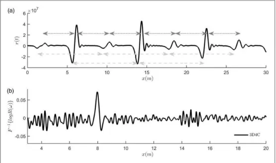
The cepstrum of the cross-correlation. Figure 5 is an example (using the 3D4C case) that demonstrates the effectiveness of the cepstrum analysis approach for extracting the periods between the delay peaks of the cross-correlation signal.
Figure 5(a) shows the cross-correlation signal, and it is possible to observe that the peaks and delay peaks are repeated within certain periods. Considering the periods of 8 m that are highlighted with dashed light grey arrows, the reason for this observation is the transient pressure wave and its reflections are trapped between inlet and leak. This period is clearly identified by the cepstrum of cross-correlation; the largest peak in Figure 5(b). Also, there is a smaller peak around
4 m in the cepstrum figure; this period is shown by the grey arrows in Figure 5(a).
When looking at Figure 3, it can be seen that the most repeated period is roughly equal to the twice distance between the inlet sensor and the leak, so there is going to be a noticeably large peak equal to twice of this distance within the cepstrum results. For a clearer presentation of the results, this periodicity has been removed in all the graphs by dividing the distances by two.
The cepstrum of cross-correlation results for differ-ent leak sizes (2D61, 2D62 and 2D65) are shown in Figure 6(a). The signal patterns are almost unaffected; however, the amplitudes varied noticeably. The high-est amplitude is observed for the larghigh-est leak size (2D65), while the smallest leak (2D61) has generated a larger amplitude signal than the medium one (2D62). It is therefore not yet possible to estimate the leak size based on the amplitude of the output signal. The smaller leak is detected with considerably higher accuracy (less than 0.6% error), while in the 2D62 case, the leak is over-predicted by about 1.8%. Figure 6(b) to (d) shows the results of the cepstrum analyses for a single leak size at different positions in the pipe from both 2D and 3D simulations, respect-ively. For both 2D and 3D cases, the analysis has shown large peaks at the distance to the leak position from the inlet. For both the 3D4C and 2D45 cases, the largest peak is located around 4 m and the leaks were detected with 0.5% and 0.75%, accuracy, respectively. Interestingly, the peak for 2D55 has cap-tured two reflections (a double peak) at this point; this could be due to the resolution and the sensor pos-itions, such that signal of the leak is spread across two time steps. The errors for identifying the leaks in 2D55 and 3D5C were 1% and 0.4%, respectively.
x(m) 5 10 15 20 25 30 35 P ( Pa ) -1000 0 1000 2000 3000 4000 5000 6000 7000 8000 9000
(a) Inlet sensor (b)
CFD Idealised x(m) 5 10 15 20 25 P ( Pa ) -100 -50 0 50 100 150 200 Outlet sensor CFD Idealised
Figure 7. Idealised inlet and outlet pressure waves simulated for a straight pipe with a leak placed 4 m upstream from the inlet compared to measured signals in the CFD simulation. CFD: computational fluid dynamics.
Finally, the peak describing the leak at 6m stream-wise is observed around 6min both 2D65 and 3D6C (0.17%). Considering the case where the leak is located at 10 m (3D10C) in Figure 6(d), the output signal can be seen to fluctuate, which is because the leak position is close to the outlet where reflections will occur. A peak can be identified at around 10 m and this leak is detected with a 1.4% error. Furthermore, the signal attenuation rate was higher in the 2D cases and double peaks were also mainly observed in 2D cases (2D62 and 2D55).
Figure 6(e) shows that the output signal for the leaks with different shapes have a very similar pattern. The output for the circular leak had more fluctuations
than the other cases, although the errors for detecting the leak were similar in all cases and equal to 0.17%. The proposed method is not sensitive to leak shape and it is able to identify leaks, regardless of their geometry.
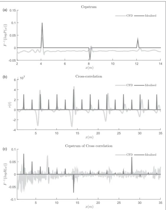
Idealised pressure signals. The signal processing meth-ods are also tested on two idealised pressure signals. It is possible to approximately estimate the time that the pressure waves are going to be sensed near the inlet and outlet of a straight pipe. Therefore, two idealised pressure signals for a straight pipe with a leak placed 4 m downstream of the inlet were created. Figure 7(a) and (b) shows the idealised inlet and outlet
x(m) 2 4 6 8 10 12 14 F − 1{ lo g P ( ω ) } -0.05 0 0.05 0.1 0.15 (a) Cepstrum CFD Idealised x(m) 5 10 15 20 25 30 35 r ( t ) ↓107 -4 -2 0 2 4 6 (b) Cross-correlation CFD Idealised x(m) 5 10 15 20 25 30 35 F − 1{ lo g R ( ω ) } -0.1 -0.05 0 0.05 0.1
(c) Cepstrum of Cross correlation
CFD Idealised
Figure 8. Idealised inlet and outlet pressure waves created for a straight pipe with a leak placed 4 m upstream from the inlet compared to measured signals in the CFD simulation. CFD: computational fluid dynamics.
pressure waves signals compared to the CFD simulation results, respectively. Note the time is converted to distance by having the speed of the pres-sure wave.
The idealised pressure signals are used to calculate cepstrum, correlation and cepstrum of cross-correlation. The results of the analysis can be found in Figure 8. Comparing the results with the CFD
simulation data shows a close estimation of the loca-tions that the peaks were expected.
Comparing the methods. Table 2 shows the numerical calculations for each case, using different signal pro-cessing methods. The first column introduces case spe-cifications, while the actual and predicted location of the leaks are given in the Xa and Xp column,
x(m) 10 20 30 40 50 60 70 80 r ( t ) ×109 -2 0 2 (a)
T-Juntion with no leak T-Junction with a leak
x(m) 5 10 15 20 25 30 35 40 F − 1{ lo g P ( ω ) } -0.02 -0.01 0 0.01 0.02 (b) x(m) 5 10 15 20 25 30 35 40 F − 1{ lo g R ( ω ) } -0.04 -0.02 0 0.02 (c)
Figure 9. The results for T-Junction cases: (a) Cross-correlation signal, (b) cepstrum and (c) cepstrum of cross-correlation. Table 2. The results of cross-correlation, cepstrum and cepstrum of cross-correlation leak detection methods.
Case Specifications Cross-correlation Cepstrum of Pressure
Cepstrum of Cross-correlation
Name Xa(m) Xp(m) Error (%) Xp(m) Error (%) Xp Error (%)
3D6LH 6 6.09 1.50 6.06 1.00 5.99 0.17 3D6TE 6 6.08 1.33 6.06 1.00 5.99 0.17 3D6C 6 6.09 1.50 6.06 1.00 5.99 0.17 3D4C 4 4.06 1.50 4.03 0.75 3.97 0.75 3D5C 5 5.07 1.40 5.04 0.80 4.98 0.40 3D10C 10 9.8 2.00 10.03 0.30 10.14 1.40 2D61 6 5.95 0.83 6.05 0.83 6.03 0.50 2D62 6 5.95 0.83 6.13 2.17 6.11 1.83 2D45 4 4.15 3.75 4.04 1.00 3.98 0.50 2D55 5 5.07 1.40 5.11 2.20 5.05 1.00 2D65 6 6.29 4.83 6.08 1.33 6.01 0.17
respectively. Finally, the errors are shown in the last column for each method.
T-Junction
Two T-Junction cases, with and without a leak were studied. Two ‘‘sensors’’ were used to capture the static pressure signal, 0.01 m after the inlet and 0.01 before the downstream outlet (outlet 2 in Figure 1). The speed of the pressure wave was estimated to be equal to 1471.7 m/s.
Figure 9(a) represents the cross-correlation out-puts. The position of the leak and the outlet can clearly be identified around 14 and 19.4 m, whilst the position of the junction is not clearly observed. On examining the cepstrum of the inlet pressure (Figure 9(b)), the position of junction, leak and outlet are all predicted with less than a 0.5% error.
The cepstrum of the cross-correlation is shown in Figure 9(c). Four sharp peaks are noticeable at the beginning of graph; the first peak, about 6 m, is related to the distance between the junction and leak-age. This peak is negative as positive reflections from the leak or a junction will give the opposite sign in the cross correlation to an open end. Furthermore, the second peak around 8.5 m identifies the junction with a 0.71% error, the third predicts the leak location (about 14.4 m) with a 0.21% error, and finally, the outlet (near 19.5 m) position is located within 0.5%. (Details of the results can be found in Table 3).
It can be seen from this that the cepstrum result is clearest for the 3D case. The accuracy of both the cepstrum and the cross correlation of the cepstrum are good with a slightly better location shown by the cepstrum. Not surprisingly, as the cepstrum of the cross-correlation should pick up the resonances within the system, it finds the distance between the leak and the junction as an additional peak. This indicates that there is a lot of information in the signals, which can be extracted using signal ana-lysis techniques.
For these more complicated systems, it may be useful to use a variety of techniques and find the common peaks to identify features with greater surety. In the cases shown above, this would be par-ticularly useful in removing the spurious peaks from the non leak analyses in Figure 9(b) and (c).
Conclusions
An improved transient leak detection method is intro-duced, which is based on the cepstrum of the cross-correlation of the signals upstream and downstream of the leak. Different leak properties are simulated within a straight pipe and a T-Junction system. This novel technique is more accurate than the cross-correlation and cepstrum results on their own for a straight pipe. However, for more complicated sys-tems, the number of peaks increases and it is harder to discern features for certain. The cepstrum of the cross-correlation method is more accurate than using the cross-correlation alone, since it picks up the periodicity in the cross correlations.
Changing the leak position in both 2D and 3D simulations showed that there was a more accurate prediction resulting from the 3D cases, showing the importance of good data for the signal analysis tech-niques. A 3D leak gives a sharper (though smaller) reflection. When the location was kept the same and the leak size was altered, the prediction error was fun-damentally unchanged. From the work shown here, there does not appear to be a straightforward method to ascertain the leak flow rate based on this method. The proposed technique is not sensitive to the leak’s geometry as it has predicted different leak shapes with roughly the same precision. It is relatively simple to pick up multiple features using this approach. For example, in the case of a T-Junction network with a leak, both features were detected with approximately a 1% error; however, it was not always clear what was a relevant peak in these more compli-cated systems.
Declaration of Conflicting Interests
The author(s) declared no potential conflicts of interest with respect to the research, authorship, and/or publication of this article.
Funding
The author(s) received no financial support for the research, authorship, and/or publication of this article.
References
1. Colombo AF, Lee P and Karney BW. A selective literature review of transient-based leak detection meth-ods.J Hydro-Environ Res2009; 2: 212–227.
Table 3. T-Junction results.
Case specification Cross-Correlation Cepstrum of Pressure Cepstrum of Cross-correlation
Name Xp(m) Xp(m) Error (%) Xp(m) Error (%) Xp(m) Error (%)
Junction 8.4 – – 8.42 0.24 8.46 0.71
Leak 14.4 14.36 0.28 14.41 0.07 14.37 0.21
Outlet 19.4 19.32 0.41 19.29 0.57 19.3 0.52
2. Wylie EB, Streeter VL and Suo L. Fluid transients in systems. vol 1, Englewood Cliffs, NJ: Prentice Hall, 1993.
3. Wylie EB and Streeter VL.Fluid transients. New York: McGraw-Hill International Book Co., 1978, p. 401. 4. Lighthill J. Waves in fluids. Cambridge: Cambridge
University Press, 2001.
5. Thorley DA. Fluid transients in pipeline systems. New York: ASME Press, 2004.
6. Beck S, Williamson N, Sims N, et al. Pipeline system identification through cross-correlation analysis. Proc IMechE, Part E: J Process Mechanical Engineering 2002; 216: 133–142.
7. Beck S, Curren M, Sims N, et al. Pipeline network fea-tures and leak detection by cross-correlation analysis of reflected waves.J Hydraul Eng2005; 131: 715–723. 8. Taghvaei M, Beck S and Staszewski W. Leak detection
in pipelines using cepstrum analysis. Measure Sci Technol2006; 17: 367–372.
9. Ghazali M, Beck S, Shucksmith J, et al. Comparative study of instantaneous frequency based methods for leak detection in pipeline networks. Mech Syst Signal Process2012; 29: 187–200.
10. Ferrante M, Brunone B and Meniconi S. Wavelets for the analysis of transient pressure signals for leak detec-tion.J Hydraul Eng2007; 133: 1274–1282.
11. Ferrante M and Meniconi S. Leak-edge detection De´tection des fuites-contours.J Hydraul Eng2009; 47: 233–241.
12. Ferrante M, Capponi C, Collins R, et al. Numerical transient analysis of random leakage in time and fre-quency domains. Civil Eng Environ Syst 2016; 33: 70–84.
13. Hanson D, Randall R, Brown G, et al. Locating leaks in underground water pipes using the complex cep-strum.Austr J Mech Eng2008; 6: 107–112.
14. Motazedi N and Beck SBM. The use of the cross-correlation of two signals as a transient leak detection method. In:BHR Group - 12th International conference on pressure surges, Dublin, Ireland, 2016, pp.581–594. 15. Le T, Watton J and Pham D. Fault classification of
fluid power systems using a dynamics feature extraction technique and neural networks.Proc IMechE, Part I: J Systems and Control Engineering1998; 212: 87–97. 16. Wiener N. Extrapolation, interpolation, and smoothing
of stationary time series. vol 2, Cambridge, MA: MIT Press, 1966.
17. Taghvaei M, Beck S and Boxall J. Leak detection in pipes using induced water hammer pulses and cepstrum analysis.Int J COMADEM2010; 19: 25.
18. Brunone B and Ferrante M. Detecting leaks in pres-surised pipes by means of transients. J Hydraul Eng 2001; 39: 539–547.
19. Lange FH and Johns P. Correlation techniques. London: Iliffe, 1967.
20. Oppenheim AV. Superposition in a class of nonlinear systems. Massachusetts: MIT Research Laboratory of Electronics, 1965.
21. Kemerait R and Childers D. Signal detection and extraction by cepstrum techniques.IEEE Trans Inform Theory1972; 18: 745–759.
22. Childers DG, Skinner DP and Kemerait RC. The cep-strum: A guide to processing. Proc IEEE 1977; 65: 1428–1443.
23. Senmoto S and Childers DG. Adaptive decompos-ition of a composite signal of identical unknown wave-lets in noise.IEEE Trans Syst Man Cybernet1972; 1: 59–66.
24. Bogert BP, Healy MJ and Tukey JW. The quefrency alanysis of time series for echoes: Cepstrum, pseudo-autocovariance, cross-cepstrum and saphe cracking. In:Proceedings of the symposium on time series analysis, New York, Vol. 15, 1963, pp.209–243.
25. Randall RB. A history of cepstrum analysis and its application to mechanical problems. In: International conference at Institute of Technology of Chartres, France, 2013, pp.11–16.
26. Hayward ATJ. Compressibility equations for liquids: a comparative study.Br J Appl Phys1967; 18: 965–977. 27. Jones WP and Launder BEi. The prediction of
laminar-ization with a two-equation model of turbulence.Int J Heat Mass Transf1972; 15: 301–314.
Appendix
Notation
2D45 2D straight pipe with a 0.005 m leak diameter at the distance of the 4 m from the inlet
2D55 2D straight pipe with a 0.005 m leak diameter at the distance of the 5 m from the inlet
2D61 2D straight pipe with a 0.001 m leak diameter at the distance of the 6 m from the inlet
2D62 2D straight pipe with a 0.005 m leak diameter at the distance of the 6 m from the inlet
2D65 2D straight pipe with a 0.005 m leak diameter at the distance of the 6 m from the inlet
3D10C 3D straight pipe with a circular leak at the distance of the 10 m from the inlet 3D4C 3D straight pipe with a circular leak at
the distance of the 4 m from the inlet 3D5C 3D straight pipe with a circular leak at
the distance of the 5 m from the inlet 3D6C 3D straight pipe with a circular leak at
the distance of the 6 m from the inlet 3DLE 3D longitudinal ellipse
3DTE 3D transverse ellipse leak
A Amplitude of the input signal CFD Computational fluid dynamics
d Leak diameter
F Fourier transform
F1 Inverse Fourier transform IFT Inverse Fourier transform
j The imaginary unit
k Data point number (index)
KW Bulk modulus
n Data point number (index)
q Static pressure at outlet sensor
Q Fourier transform of the input signal
r Cross-correlation Re Reynolds number
TCP T-Junction case with a circular leak
X The distance of the leak from the inlet
! Frequency
Density
Phase
Results independency from the sensor positions
To check the independency of the results from the sensor positions, four different sensors positioned
0.01, 0.02, 0.04 and 0.1 m downstream of the outlet of the T-Junction case were created. As Figure 10 demonstrates the shifting, the position of the outlet sensor does not affect the general pattern of the signal and the associated cepstrum results. However, it is possible to see that, due to the position of the sensor, a number of double peaks are generated in the cross-correlation of the signal. Considering the area between 45 and 65 m, a double peak is cap-tured by the sensors placed at 0.01 and 0.02 m, whilst this phenomena is not seen in the 0.04 and 0.1 m sensors. x(m) 0 20 40 60 80 100 120 140 160 180 200 r ( t ) ×1013 -8 -6 -4 -2 0 2 4 6 (×14) 0.01 m (×2) 0.02 m 0.04 m (×2)0.1 m