DRO
Deakin Research Online,
Deakin University’s Research Repository Deakin University CRICOS Provider Code: 00113B
A classifier graph based recurring concept detection and prediction approach
Citation:
Sun, Yange, Wang, Zhihai, Bai, Yang, Dai, Honghua and Nahavandi, Saeid 2018, A classifier
graph based recurring concept detection and prediction approach
, Computational
intelligence and neuroscience
, vol. 2018, Article ID: 4276291, pp. 1-13.
DOI:
http://www.dx.doi.org/10.1155/2018/4276291
© 2018, The Authors
Reproduced by Deakin University under the terms of the
Creative Commons Attribution Licence
Downloaded from DRO:
Research Article
A Classifier Graph Based Recurring Concept Detection and
Prediction Approach
Yange Sun
,
1,2Zhihai Wang
,
1Yang Bai,
1Honghua Dai,
3and Saeid Nahavandi
41School of Computer and Information Technology, Beijing Jiaotong University, Beijing 100044, China 2School of Computer and Information Technology, Xinyang Normal University, Xinyang 464000, China 3Deakin University, Melbourne, VIC 3125, Australia
4Institute for Intelligent Systems Research and Innovation, Deakin University, Waurn Ponds, VIC 3220, Australia
Correspondence should be addressed to Zhihai Wang; [email protected]
Received 27 October 2017; Revised 15 January 2018; Accepted 19 April 2018; Published 7 June 2018
Academic Editor: Christian W. Dawson
Copyright © 2018 Yange Sun et al. This is an open access article distributed under the Creative Commons Attribution License, which permits unrestricted use, distribution, and reproduction in any medium, provided the original work is properly cited.
It is common in real-world data streams that previously seen concepts will reappear, which suggests a unique kind of concept drift, known as recurring concepts. Unfortunately, most of existing algorithms do not take full account of this case. Motivated by this challenge, a novel paradigm was proposed for capturing and exploiting recurring concepts in data streams. It not only incorporates a distribution-based change detector for handling concept drift but also captures recurring concept by storing recurring concepts in a classifier graph. The possibility of detecting recurring drifts allows reusing previously learnt models and enhancing the overall learning performance. Extensive experiments on both synthetic and real-world data streams reveal that the approach performs significantly better than the state-of-the-art algorithms, especially when concepts reappear.
1. Introduction
In recent years, with the technological advance, a grow-ing number of applications produce large amounts of data streams at high speed. Examples include sensor networks, spam filtering systems, traffic control, and intrusion detection [1, 2]. More formally, a data stream S is a potentially unbounded, ordered sequence of instances, which arrive continuously at high-speeds.
One of the biggest challenges in data stream learning is to deal with concept drift [3–5], i.e., the underlying concept may drift dynamically over time. Concept drift frequently occurs in the real world. For example, in recommend systems, user consumption preferences may change over time due to fashion, economy, and so on and weather prediction models may change according to the seasons. Such changes lead to a drastic drop in classification performance. A reasonably useful classifier should have the capability to recognize and respond to such changes accordingly and accurately. This study focuses on the topic of developing classifier learn-ing systems for minlearn-ing data streams in dynamic environ-ments.
Concept drift can be divided depending on their speed, into sudden and gradual drifts [4]. Sudden concept drift is characterized by large amounts of changes between the underlying class distribution and the incoming instances in a relatively short amount of time. Gradual concept drift can take a very large amount of time to see a significant change in differences of underlying class distributions between the old instances and the incoming instances. In fact, no matter what type of change occurs, the model should be able to track and adapt to changes accordingly.
It is common that in real-world data streams previously seen concepts may reappear in the future. For example, weather prediction models change according to the seasons and a popular topic may appear in a social network during the time of the year (i.e., festivals or elections) [4, 6]. This demonstrates a unique kind of drift, known as recurring concepts [6]. For example, news reading preference of a user may change over time. A user can have different choices on mornings, evenings, weekdays, and weekends. In addition, a user might search for astrology articles in the beginning of the year and financial articles at the beginning of each quarter. Unfortunately, only few approaches take recurring concepts
Volume 2018, Article ID 4276291, 13 pages https://doi.org/10.1155/2018/4276291
data mean
(a) Sudden concept drift (b) Gradual concept drift (c) Recurring concept drift
Figure 1
into consideration [6–8]. In the situation where concept may recur, the classification models which have been used in the past may apply to the future use. However, most existing papers on drift detection neglect this phenomenon and tend to take the concept which occurs after a drift as a new one.
If a concept reappears, the previously learnt classifiers should be reapplied; thus the performance of the learning algorithm can be improved. This study focuses on the problem of recurring concepts. Two crucial problems will be addressed:(1)How to detect the recurring concepts.(2)How to effectively adapt when a recurring concept is detected.
Due to the fact that drift detection can capture changes in data streams timely and then update the predictive model, the predictive model can maintain high accuracy. Following these critical motivations, an efficient scheme is designed to deal with the above issues. The key contribution of our algorithm is threefold:
(1) A Drift Detection Method named Distribution-Based Detection Method (DBDM) is introduced aiming at addressing the first issue. It detects changes by comparing the distribution of data in different time windows based on Bernstein inequality.
(2) An algorithm named the Recurrent Detection and Prediction (RDP) approach is introduced targeting on solving the second problem. It stores concepts which present previ-ously occurred concepts with a graph model.
(3)The performance comparison results of the proposed algorithms evaluated on a variety of datasets demonstrated that our method is both stable enough on the data streams with gradual concept drifts and flexible enough to adapt effec-tively to sudden concept drifts and the recurring concepts problem.
The rest of the paper is as follows. Section 2 reviews the related work. In Section 3, we discussed the basic ideas of the presented algorithms in detail. Section 4 provided the experimental results tested on both real and synthetic datasets followed by analysis and discussions. In the last section, we draw conclusions and discussed future work.
2. Related Work
In this section, first, some relevant concepts will be intro-duced, then, several related algorithms will be reviewed, and finally, based on these previous works, the original contributions of the paper will be summarized.
2.1. Basic Concepts and Notations
Definition 1(data streams). LetSbe an infinited-dimensional data stream
𝑆 = {(𝑥1, 𝑦1) , (𝑥2, 𝑦2) , . . . , (𝑥𝑡, 𝑦𝑡) , . . .} . (1)
Each instance is a pair (xt,yt), wherextis a vector of attribute
values arriving at the time stamptandytis the class label of
xt.
Definition 2 (concept drift). The term concept drift can be formally defined as any scenario where the joint probability, which represents data distribution, changes over time, i.e.,
𝑃𝑡(𝑥𝑖, 𝑦𝑖) ̸= 𝑃𝑡+1(𝑥𝑖, 𝑦𝑖)[9].
Definition 3(sudden concept drift). As shown in Figure 1(a), sudden concept drift means that the distribution of data will be changed directly to a new one in a relatively short time.
Definition 4(gradual concept drift). As shown in Figure 1(b), gradual concept drift means that the probability of the old data distribution will decrease and the probability of a new distribution will increase during a very large amount of time to see a significant change.
Definition 5 (recurring concept drift). As shown in Fig-ure 1(c), a recurring concept drift occurs when the instances from a periodkare generated from the same distribution as a previously observed periodPk(xi,yi) =𝑃𝑘-𝑗(xi,yi).
Definition 6(classifier graph). A classifier graph is a graph whose nodes are stored with distinct classifiers derived from a given stream data. Each node in a classifier graph stores a classifier; directed link represents a drift; weight of a link represents drifting times.
2.2. Handling Concept Drift in Data Streams. Approaches to cope with concept drift can be divided into two main categories: passive and active approaches [5, 10]. The first approach adapts a learner at regular intervals without con-sidering whether changes have really occurred, and it tracks changes blindly and updates the model continuously with-out requiring explicit change detection, while the second approach only makes adjustment when a drift occurs.
Active approaches typically require change detection modules. Gama et al. [11] presented a Drift Detection Method (DDM) which detects change by monitoring the classification error rate. Baena-Garcia et al. [12] introduced a detection algorithm called Early Drift Detection Method (EDDM) which has a better performance in the scenario of gradual change. Adaptive Windowing (ADWIN) [13] adopted a sliding window to store instances recently read and divides the window into two subwindows to monitor changes in the subwindows. EWMA for Concept Drift Detection (ECDD) was introduced by Ross et al. [14], which uses exponen-tially weighted moving average charts to monitor the error rate. Sakthithasan et al. [15] proposed an algorithm named
SeqDrift which adopts reservoir sampling to manage the memory and improve the detection sensitivity in the case of slow gradual change.
Ensemble classifiers are one of the most popular passive approaches, and many active approaches based on ensemble are available in the literature. Streaming Ensemble Algorithm (SEA) [16] is one of the earliest solutions which adopt an ensemble strategy to address concept drift. It makes final pre-diction using a simple majority voting. Accuracy Weighted Ensemble (AWE) [17] is similar to SEA. It decides the weight of base leaner according to the classification accuracy of the learner on test datasets. Dynamic Weighted Majority algorithm (DWM) [18] is an ensemble based on the weighted majority mechanism and each classifier corresponds to a weight which can change dynamically. Online Coordinate Boosting (OCBoost) [19] is an online boosting algorithm, which adopts online boosting strategy to achieve a better performance. Diversity for Dealing with Drifts (DDD) [20] is a novel ensemble method which maintains ensembles with different levels of diversity.
While active approaches, such as change detection, work quite well in coping with sudden concept drift, passive approaches work better for gradual drift which is neverthe-less more difficult to detect. In order to react to different types of concept drifts immediately, some approaches try to utilize both passive and active techniques to aid learn-ing in nonstationary environments, which seek to combine the best elements of both passive approaches and active approaches.
As we pointed out earlier it is very common in real-world data streams that previously seen concepts will reappear. This suggests a unique kind of concept drift, known as recurring concepts. However, none of the aforementioned approaches take the problem of Recurring Concept Drifts into account. The concept of Recurring Concept Drifts has been introduced by Widmer et al. In [8], Katakis et al. presented a framework to detect recurring contexts. In this framework, batches of instances are mapped into concep-tual vectors and stream clustering is used to group these conceptual vectors into different clusters. Then incremental classifiers are trained for every cluster. When a new batch of instances arrives, it was assigned into an existing clus-ter or a new clusclus-ter is created for it. Gomes et al. [21] introduced a data stream learning system which exploited context information to add and delete classifiers in the ensemble to improve existing ensemble approaches to deal with concept drift and recurring concept. Abad et al. [22] devised a framework to solve the issue of recurring concept in spam filtering. The framework handles the context which is related to concept drift. Gonc¸alves et al. [23] presented a framework named Recurring Concept Drifts (RCD) to handle recurring concept drift. In the framework, the new classifier is created when new concept occurs and a group of instances corresponding to the new concept is stored. When a new drift is detected, RCD compares the incoming instances with the previous ones to validate whether the two sets of instances come from the same distribution. If they are from the same distribution, the previous classifier is reused.
3. Learning Recurring Concept from
Classifier Graph
In this section, a novel change detection paradigm based on the distribution between two subwindows will be introduced first, and then an internal classifier graph empowered drift detection mechanism will be presented in detail.
3.1. Change Detection Problem. Let W1= (xt+1, . . ., xt+n)
denote reference window, letW2= (xt+n+1,. . .,xt+2n)
repre-sent current window, let̂𝜇𝑊1and ̂𝜇𝑊2be the average value of
W1 andW2, and let 𝜇W1 and𝜇W2 be their expected value.
In fact, the underlying distribution of data is unknown and a test statistic based on sample means needs to be adopted by the change detector. This is accomplished by carrying out statistical tests that verifies whether the classification error or class distribution remains constant over time. The problem of change detection in data streams is to determine the null hypothesisH0against alternative hypothesisH1as follows:
𝐻0 Pr(̂𝜇𝑊1, ̂𝜇𝑊2 ≥ 𝜀) ≤ 𝛿
𝐻1 Pr(̂𝜇𝑊1, ̂𝜇𝑊2 ≥ 𝜀) > 𝛿
(2)
where𝛿 ∈ (0, 1)is a confidence value, while𝜀is a function of
𝛿when test statistics are used to model the difference between the means of instance in two windows. The change detection raises a change alarm, when the difference is greater than a threshold.
3.2. Distribution-Based Change Detection Using Bernstein Inequality. In this paper, a Distribution-Based Detection Method (DBDM) was presented by comparing the distri-bution of data in different time windows. The two-window paradigm is exploited by comparing error rate of the classi-fiers extracted from old and recent data. A correct prediction can be considered to be 1 and incorrect prediction to be 0. In the change detection, windows contain simple information (bits or numbers); thus the change tests are really simple. The sliding windowWwas partitioned into two equal length subwindows: a left subwindowW1and a right subwindowW2
with means 𝜇1 and𝜇2, respectively. Whenever the amount of new data reachesm, the boundary between the new data and the data arrived before it is taken as a check point. Then every check point is traversed to check whether the difference between the mean value of the data in the left subwindow of the check point and that of the right subwindow is greater than a threshold.
The key to the detection method is the calculation of the threshold𝜀. The inequalities which are often used to depict the difference between two distributions are Hoeffding inequality [24], Chernoff inequality [25], and Bernstein inequality [26]. Among them, the Hoeffding inequality is widely used in pre-vious research. However, the Hoeffding inequality neglects the effect of variance, which leads to imprecise results in the case of small variance. Bernstein inequality associates expected value with variance. For this reason, a more precise
threshold can be obtained by using Bernstein inequality. It is defined as follows: Pr( 1 𝑛 𝑛 ∑ 𝑖=1 𝑋𝑖− 𝐸𝑋 ≥ 𝜀) ≤ 2exp( −𝑛𝜀 2 2𝜎2+ (2/3) 𝜀 (𝑐 − 𝑎)) (3)
where𝑋1, 𝑋2, ⋅⋅⋅, 𝑋𝑛are independent random variables,𝑋𝑖∈
[𝑎, 𝑐],𝐸𝑋is the expected value, and𝜎2is the variance. The probability of capturing concept drift at a certain check point is no more than𝛿, which can be expressed as shown in
Pr[̂𝜇1− ̂𝜇2 ≥ 𝜀] ≤ 𝛿 (4)
Applying Boole’s inequality, (4) can be converted into Pr[̂𝜇1− ̂𝜇2 ≥ 𝜀] ≤Pr[̂𝜇1− 𝜇 ≥ 𝑘𝜀]
+Pr[̂𝜇2− 𝜇 ≥ (1 − 𝑘) 𝜀] (5) wherekis the proportion of data among the left and right side.
Apply Bernstein inequality on the RHS of (5): Pr[̂𝜇1− ̂𝜇2 ≥ 𝜀] ≤ 2exp( −𝑛1(𝑘𝜀) 2 2𝜎12+ (2/3) 𝑘𝜀 (𝑐 − 𝑎)) + 2exp( −𝑛2[(1 − 𝑘) 𝜀] 2 2𝜎22+ (2/3) (1 − 𝑘) 𝜀 (𝑐 − 𝑎)) (6)
where𝜎12and𝜎22represent variances. By substitutingaand
cwith 0 and 1 in (6), we obtain
Pr[̂𝜇1− ̂𝜇2 ≥ 𝜀] ≤ 2exp( −𝑛1(𝑘𝜀) 2 2𝜎12+ (2/3) 𝑘𝜀) + 2exp( −𝑛2[(1 − 𝑘) 𝜀] 2 2𝜎22+ (2/3) (1 − 𝑘) 𝜀) = 𝛿 (7)
It is worth noting that formulation of the optimization problem for determiningkis based on asymptotic behavior and so thatk’s value is approximate. Equating the two terms in expression yields
𝑛1𝜎1= 𝑛2𝜎2 (8)
Let𝛿in (7) be equated to the user-assigned𝛿and set the two exponents to be equal. We have
𝛿 = 4exp( −𝑛1[(1 − 𝑘) 𝜀] 2 2𝜎12+ (2/3) (1 − 𝑘) 𝜀) = 4exp( −𝑛1[(1 − 𝑘) 𝜀] 2 2 (𝑛1𝜎12/𝑛 2) + (2/3) (1 − 𝑘) 𝜀) (9)
We have equated 𝛿 to the left exponential term in (7) instead of the right one to get𝜀. We have
𝜀 = 1 3𝑛1𝑘(ln 4 𝛿+ √(ln 4 𝛿) 2 + 18𝑛1𝜎12ln4 𝛿) (10)
We set 𝛿𝑤𝑎𝑟𝑛𝑖𝑛𝑔 and 𝛿𝑑𝑟𝑖𝑓𝑡, and then 𝜀𝑤𝑎𝑟𝑛𝑖𝑛𝑔 and 𝜀𝑑𝑟𝑖𝑓𝑡 can be calculated. When the difference of the mean values is greater than𝜀𝑤𝑎𝑟𝑛𝑖𝑛𝑔, meaning that a drift has been triggered. And when difference of the mean values is greater than𝜀𝑑𝑟𝑖𝑓𝑡, we confirm that the concept has been changed.
In DBDM, before an actual change point is detected multiple check points need to be detected. In multiple testing problems, as the number of hypotheses being tested increases, the likelihood of incorrectly rejecting a null hypothesis increases. Most of the existing algorithms adopt Bonferroni correction [27] to avoid the problem. However, Bonferroni correction is less effective when there are a large number of tests. For this reason, we adopt the error correction factor based on ˇSid´ak correction [28].𝛿𝑠is modified according to
𝛿𝑠= 1 − (1 − 𝛿)1/√𝑛 (11)
wherendenotes the number of hypotheses. The pseudocode is presented in Algorithm 1.
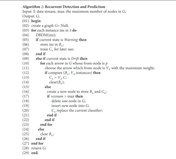
3.3. Recurrent Detection and Prediction Approach. In this section, we design a novel triggered rebuild approach named Recurrent Detection and Prediction (RDP) approach that uses a weighted directed graph to predict which previously occurred concept is the most likely to recur when a new concept drift is detected.
In RDP, the recurring concepts and corresponding instances will be stored. Directions and weights of the arrows indicate the transformation relation of the concepts stored in graph. Whenever the change detection reaches the warning level, a set of instances will be stored and a new classifier will be trained. When the state is transformed into drift, verification will be carried out to see whether the latest stored instances and instances which have been stored in graph are same. If they are drawn from the same distribution, the current concept will be regarded as a recurring concept. Then the stored instances in classifier will be utilized in order to replace the current classifier. Otherwise, we regard that a concept has occurred. Then a new classifier is trained and the set of instances are in a graph.
As defined in classifier graph, each node stores a classifier and a set of instances used to induce the classifier. When concept drifts occur, one will be added to the weight of the arrow whose to-node is the new concept and the from-node is the concept occurring before the drift. And next time when a drift is detected, classifier graph can be employed to predict which previously occurred concept is the most likely to recur this time. The algorithm is illustrated in detail with an example as Figures 2–5.
As shown in Figure 2, provided that the current concept is concept 1, we can detect concept drift after a period of
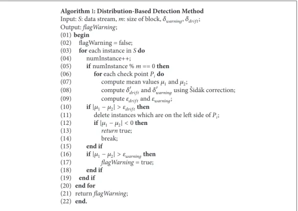
Algorithm1: Distribution-Based Detection Method
Input:S: data stream,m: size of block,𝛿𝑤𝑎𝑟𝑛𝑖𝑛𝑔,𝛿𝑑𝑟𝑖𝑓𝑡; Output:flagWarning;
(01)begin
(02) flagWarning = false;
(03) foreach instance inSdo (04) numInstance++;
(05) ifnumInstance %m== 0then (06) foreach check pointPido
(07) compute mean values𝜇1and𝜇2;
(08) compute𝛿𝑑𝑟𝑖𝑓𝑡and𝛿𝑤𝑎𝑟𝑛𝑖𝑛𝑔using ˇSid´ak correction;
(09) compute𝜀𝑑𝑟𝑖𝑓𝑡and𝜀𝑤𝑎𝑟𝑛𝑖𝑛𝑔;
(10) if|𝜇1− 𝜇2| > 𝜀𝑑𝑟𝑖𝑓𝑡then
(11) delete instances which are on the left side ofPi;
(12) if|𝜇1− 𝜇2| < 0then (13) returntrue; (14) break; (15) end if (16) if|𝜇1− 𝜇2| > 𝜀𝑤𝑎𝑟𝑛𝑖𝑛𝑔then (17) flagWarning= true; (18) end if (19) end if (20) end for (21) returnflagWarning; (22) end.
Algorithm 1: The pseudocode of DBDM.
concept 1 concept 2 concept 3 concept 4 concept 5 2 2 1 4 1 5
Figure 2: Classifier graph diagram.
time. Because the arrow directed from concept 1 to concept 3 has the maximum weight among the arrows whose from-node is concept 1, we assume that concept 3 recurs this time. If it is false, we choose the arrow whose weight is the second maximum. The procedure will be repeated. If all arrows whose from-node is concept 1 which does not recur this time, then the node which is not the one of to-node of concept 1, i.e., concept 5, will be checked to see whether it is a recurring concept. There are three cases:
(1)Concept 2, concept 3, or concept 4 recurs this time. We assume that concept 2 recurs, and then we add the weight of the arrow from concept 1 to concept 2, as shown in Figure 3.
concept 1 concept 2 concept 3 concept 4 concept 5 2 3 1 4 1 5
Figure 3: Concept 2 recurs.
(2) As shown in Figure 4, concept 5 is the recurring concept. An arrow will be added from concept 1 to concept 5.
(3)When a new concept 6 occurs, a node will be created and an arrow will be added from concept 1 to concept 6, as shown in Figure 5.
Let G represent the graph, V is the set of vertexes in
G, vexnumdenotes the serial number of vertexes inG, Cn
is a new classifier which applies to the new concept,Vk.C
represents the previous classifier ofVk.Bnrepresents a set of
instances which corresponding to new concept, andpis the order of the old concept inG. The pseudocode of RDP is listed in Algorithm 2.
concept 1 concept 2 concept 3 concept 4 concept 5 2 1 4 5 2 1 1
Figure 4: Concept 5 recurs.
concept 1 concept 2 concept 3 concept 4 concept 5 2 2 1 4 5 concept 6 1 1
Figure 5: New concept occurs.
4. Experiment Results and Analysis
The algorithms were carried out with help of MOA (Massive Online Analysis) (Version: MOA Release 2017.7) [29]. MOA is a software environment for implementing algorithms and running experiments for online learning. All of the experiments were performed on an Intel Core i3-2120 CPU @ 3.3GHz with 8GB of RAM running Windows 7.
To evaluate the performance of the proposed algorithms, a series of experiments were carried out. Two main sets of experiments are presented:
Experiment 1 aims to verify the fact that the performance of the proposed change detection in different drift scenarios. Experiment 2 is set to compare the performance of the RDP with other state-of-the-art approaches.
4.1. The Analysis of DBDM. In the first experiment, the performance of DBDM is compared against the following algorithms: DDM [11], EDDM [12], and ECDD [14] in terms of the false positive counts. In DBDM, we set𝛿𝑑𝑟𝑖𝑓𝑡 = 0.1,
𝛿𝑑𝑟𝑖𝑓𝑡 = 0.1and the size of block is 500. In ECDD, we set
ARL0=1,000 and𝜆 = 0.2.
We generated four datasets. Each has 200,000 instances which were drawn from a stationary Bernoulli distribution and the mean value of the Bernoulli distribution is set to 0.05,
Table 1: Average false positive counts on stationary Bernoulli distribution. 0.05 0.1 0.3 0.5 DDM 1.89 0.76 0.29 0.19 EDDM 35.56 36.3 14.42 9.38 ECDD 166.34 157.3 154.01 0.11 DBDM 3.39 0.95 0.05 0.03
Table 2: Average false positive counts on sudden concept drift.
mean value increment 0.04 0.09 0.29 0.49
DDM 11.93 10.06 8.34 8.7
EDDM 46.00 45.14 32.63 25.17 ECDD 173.81 169.55 168.07 91.43
DBDM 4.99 3.76 7.69 9.77
Table 3: Detection delays on an abrupt drift.
mean value increment 0.04 0.09 0.29 0.49 DDM 3823.96 1817.97 419.66 300.92 EDDM 1758.95 759.96 221.06 148.59
ECDD 528.61 497.99 522.97 426.8
DBDM 529.29 235.64 200 200
0.1, 0.3, and 0.5, respectively [13]. To make the experimental more reliable, the algorithms were carried out on each dataset for 10 times and then calculated the mean.
Table 1 shows that the false positive count of DBDM is lower than EDDM and ECDD, but it is higher than DDM. It also demonstrates that the false positive count of DBDM is reduced from 3.39 to 0.03 with the increase of the mean value of Bernoulli distribution.
Then, we compared the performance of detectors under sudden concept drift scenario. We generated four datasets of 200,000 instances drawn from a Bernoulli distribution. The first 100,000 instances were drawn from stationary Bernoulli distribution whose mean value was 0.01. And the mean of the last 100,000 instances was raised to 0.05, 0.1, 0.3, and 0.5 for the four datasets separately.
Table 2 shows that the false detection of DBDM is the lowest when the change of the mean is small. However, the false positive rate of DBDM is increased with the increase of the mean value.
Table 3 shows the average detection delays under sudden concept drift. In general, the detection delays decrease with the increase of the mean value. The detection delay of DDM is higher when the mean value increment is low, and then it decreases rapidly. The detection delay of EDDM is high when the mean value increment is 0.04, and then it decreases gradually. At the beginning, the delay of ECDD is lower than DDM and EDDM, and then it drops slightly. However, the delay of ECDD increases when the mean value of increment is 0.29. The detection delay of DBDM is lower and it has a downward trend. This is due to the fact that the management of the recurrent change detection mechanism is capable of reusing previous concepts and gains
Algorithm2: Recurrent Detection and Prediction
Input:S: data stream, max: the maximum number of nodes inG; Output:G;
(01) begin
(02) create a graphG= Null;
(03) foreach instance ins inSdo (04) DBDM(ins);
(05) ifcurrent state isWarningthen (06) store ins inBn;
(07) trainCnfor later use;
(08) end if
(09) else ifcurrent state isDriftthen
(10) foreach arrow inGwhose from-node isp
(11) choose the arrow which from-node isVkwith the maximum weight;
(12) ifcompare (Bn,Vk.instances)then
(13) Cn=Vk.C;
(14) clear(Bn);
(15) else
(16) create a new node to storeBnandCn;
(17) ifvexnum>maxthen (18) delete one node inG;
(19) insert new node intoG;
(20) Cnreplace the current classifier;
(21) end if (22) end if (23) end for (24) else (25) clearBn; (26) end if (27) end for (28) returnG; (29) end.
Algorithm 2: The pseudocode of RDP.
the better performance in different situations, particularly under concept drift environments.
Finally, we investigated the performances of the four detection methods in the scenario of gradual change. When drift happens incrementally, the change is not obvious. Therefore, we mainly focus on detection delay and false negative. Detection delay is the distance between the instance at which the change is detected and the instance at which the change really occurs. In the experiment, we generate a dataset contains 1,000,000 instances. The first 998,000 instances are stable, and the mean value is 0.01. Then mean values of the last 2,000 instances of the four datasets rise with a different slope separately. The slopes are 0.0001, 0.0002, 0.0003, and 0.0004. The false negative counts are as shown in Table 4. The false negative counts of ECDD and DBDM are 0. And the false negative counts of DDM and EDDM decrease with the increase of the slope.
The detection delays are demonstrated in Table 5. It can be seen that DDM and EDDM are not good at detecting gradual drift. ECDD is rather high, although it reduces a little with the increase of the slope. DBDM is high at the beginning, but it reduces obviously with the increase of the slope. It demonstrates that DBDM is superior to other methods. It is partly because the management of the recurrent change
Table 4: Average false negative counts on a gradual drift.
Slope 0.0001 0.0002 0.0003 0.0004
DDM 0.75 0.58 0.51 0.32
EDDM 0.98 0.97 0.91 0.83
ECDD 0 0 0 0
DBDM 0 0 0 0
Table 5: Detection delays on a gradual drift.
Slope 0.0001 0.0002 0.0003 0.0004
DDM -- -- --
--EDDM -- -- --
--ECDD 523.55 508.5 515.58 509.25
DBDM 702 454 330 328
detection mechanism is capable of reusing historical concepts and achieving the better performance in this scenario.
4.2. Comparative Performance Study. This part demonstrates the experimental results with regard to the effectiveness and efficiency of the proposed method.
Table 6: Description of the nine datasets.
Dataset Instances Attributes Drift type Noise
HyperPlane 1M 10 gradual 5%
LED 1M 24 sudden 15%
Random Tree 1M 10 recurring 0%
SEA 1M 3 sudden recurring 10%
Elist 1, 500 913 recurring
-Spam 9, 324 850 gradual
-Usenet 5, 931 658 unknown
-Covertype 581K 53 unknown
-Gas Sensor 13, 910 128 unknown
-Table 7: Characteristics of Elist.
1-300 300-600 600-900 900-1200 1200-1500
Medicine + -- + - +
Space -- + -- +
--Baseball -- + -- +
--4.2.1. Datasets. In the second experiment, we adopted four synthetic and five real-world datasets. The datasets are sum-marized in Table 6.
Synthetic Datasets. In the experiment, the synthetic datasets contain three types of concept drift: gradual, sudden, and recurring concept drift.
HyperPlane dataset is represented by the set of pointsx
that satisfy∑𝑑𝑖=1𝑤𝑖𝑥𝑖= 𝑤0, wherex𝑖is theith coordinate ofx. Two classes are distinguishing in the following way: instances for which∑𝑑𝑖=1𝑤𝑖𝑥𝑖 ≥ 𝑤0are labeled positive and instances for which ∑𝑑𝑖=1𝑤𝑖𝑥𝑖 < 𝑤0 are labeled negative. Drifts was introduced by changing each weight attribute𝑤𝑖=𝑤𝑖+d𝜎, where 𝜎 is the probability that the direction of change is reversed anddis the change applied to every instance. This generator was adopted to create a dataset contains 1,000,000 instances with gradual drifts by the modification weight𝑤𝑖 changing by 0.001 with each instance, and 5% noise was added to streams.
LED dataset is to predict the digit displayed on a seven-segment LED display. The particular configuration of the gen-erator used for the experiment produces 24 binary attributes, 17 of which are irrelevant. Concept drift is simulated by interchanging relevant attributes. We generated a stream of 1,000,000 instances with sudden concept drifts and 15% of noise.
Random Tree dataset is generated by Random Tree gen-erator and it contains 1,000,000 instances and 10 attributes. It has four recurring concepts which evenly distributed throughout the 1,000,000 instances.
SEA dataset consists of three attributes, where only two are a relevant attributes. All three attributes have values between 0 and 10. The points of the dataset are divided into four blocks with different concepts. In each block, the classification is done usingf1 + f2 ≤ 𝜃, where f1 and f2 represent the first two attributes and𝜃 is a threshold value. The most frequent values are 9, 8, 7, and 9.5 for the data blocks.
It contains 1,000,000 instances with sudden drifts reappearing every 250,000 instances and 10% of noise.
Real-World Datasets. Real-world stream environment conceptual changes have unpredictability and uncertainty which can better verify the performance of the algorithm.
Emailing list (Elist) contains a stream of emails on various topics which are shown to the user one after another and are marked as interesting or junk. It is composed of 1, 500 instances with 913 attributes and is divided into 5 periods every 300 instances. At the end of each period, the user’s interest in a topic changes in order to simulate the occurrence of concept drift. Thus, the transformation between two periods is a signal of drift. The dataset can be obtained at http://mlkd.csd.auth.gr/concept drift.html. The characteristics of Elist are presented in Table 7, where (+) means an interested email and (--) indicates a spam.
Spam dataset represents the scenario of gradual concept drift and is based on the Spam Assassin Collection [8] available in http://spamassassin.apache.org/. It consists of 9, 324 instances with 500 attributes.
Usenet dataset simulates a news filtering system with the presence of concept drifts relative to the change of interest of a user over time [8]. The dataset contains 5,931 instances representing documents collected from the 20 Newsgroups. It is available at http://www.liaad.up.pt/kdus/products/data-sets-for-concept-drift.
Covertype dataset from UCI archive [30] contains 581,012 instances, 54 attributes, and no missing values. The aim is to predict the forest cover type based on cartographic variables. It can be obtained at http://moa.cms.waikato.ac.nz/datasets/, and then we simulated the dataset into streams by the MOA generators.
Gas Sensor Drift Dataset also from UCI archive contains 13,910 measurements from 16 chemical sensors utilized in simulations for drift compensation in a discrimination task of 6 gases at various levels of concentrations. The dataset was gathered within January 2007 to February 2011 (36 months)
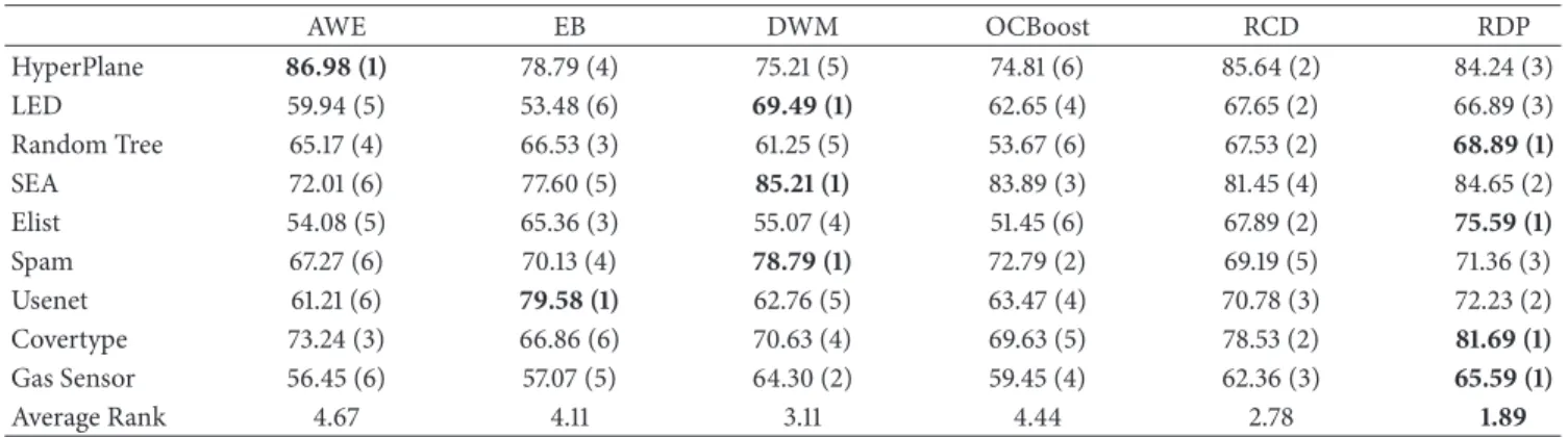
Table 8: Comparison of classification accuracy (%). AWE EB DWM OCBoost RCD RDP HyperPlane 86.98 (1) 78.79(4) 75.21(5) 74.81(6) 85.64(2) 84.24(3) LED 59.94(5) 53.48(6) 69.49 (1) 62.65(4) 67.65(2) 66.89(3) Random Tree 65.17(4) 66.53(3) 61.25(5) 53.67(6) 67.53(2) 68.89 (1) SEA 72.01(6) 77.60(5) 85.21 (1) 83.89(3) 81.45(4) 84.65(2) Elist 54.08(5) 65.36(3) 55.07(4) 51.45(6) 67.89(2) 75.59 (1) Spam 67.27(6) 70.13(4) 78.79 (1) 72.79(2) 69.19(5) 71.36(3) Usenet 61.21(6) 79.58 (1) 62.76(5) 63.47(4) 70.78(3) 72.23(2) Covertype 73.24(3) 66.86(6) 70.63(4) 69.63(5) 78.53(2) 81.69 (1) Gas Sensor 56.45(6) 57.07(5) 64.30(2) 59.45(4) 62.36(3) 65.59 (1) Average Rank 4.67 4.11 3.11 4.44 2.78 1.89
Table 9: Comparison of time consumption (Cpu seconds).
AWE EB DWM OCBoost RCD RDP HyperPlane 13.47 (1) 14.40(2) 59.01(5) 153.08(6) 29.21(3) 35.35(4) LED 20.98(5) 31.36(6) 10.51 (1) 12.43(3) 19.98(4) 11.24(2) Random Tree 37.42(3) 38.18(4) 49.53(5) 78.13(6) 31.42(2) 30.24 (1) SEA 36.41(5) 44.56(6) 20.01(2) 13.87 (1) 26.41(4) 24.05(3) Elist 17.36(2) 33.45(5) 50.21(6) 22.23(4) 20.11(3) 7.02 (1) Spam 81.43(4) 63.01(2) 85.23(5) 86.36(6) 60.43 (1) 80.25(3) Usenet 20.21(2) 26.69(3) 30.21(5) 30.78(6) 28.01(4) 16.69 (1) Covertype 26.41(4) 13.43(2) 36.06(5) 41.56(6) 6.41 (1) 14.67(3) Gas Sensor 86.57(3) 90.12(4) 97.79(6) 96.41(5) 80.12(2) 71.21 (1) Average Rank 3.22 3.56 4.44 4.78 2.67 2.11
in a gas delivery platform facility situated at the Chemo Signals Laboratory in the Bio Circuits Institute, University of California San Diego.
4.2.2. Comparative Study. We compared RDP with five ensemble-based methods: Accuracy Weighted Ensemble (AWE), Ensemble Building (EB), Dynamic Weighted Major-ity (DWM), Online Coordinate Boosting (OCBoost), and Recurring Concept Drifts (RCD). AWE is the best-known representative of block-based ensembles for data streams. Similar to AWE, EB constructs a subset of classifiers from sequential data chunks and then are used in the ensemble. DWM is based on the weighted majority algorithm, which maintains an ensemble of classifiers and each classifier corre-sponds to a weight which can change dynamically. OCBoost is an online boosting algorithm. RCD is a framework to deal with recurring concept drift.
The performance of the analyzed algorithms can be evaluated with respect to accuracy, time efficiency, memory usage, and F1-measure. The results are shown in Tables 8–11. F1-measure represents a harmonic mean between recall and precision. The calculation equation is as follows:
F1= 2 ×Re𝑐𝑎𝑙𝑙 ×Pr𝑒𝑐𝑖𝑠𝑖𝑜𝑛
Re𝑐𝑎𝑙𝑙 +Pr𝑒𝑐𝑖𝑠𝑖𝑜𝑛 (12)
(1) In terms of accuracy, as shown in Table 8, RDP makes the overall best performance on most of datasets. Specifically, RDP demonstrates significantly the best results
on the data steams with recurrent concept drift (Random Tree and Elist). On the dataset with gradual concept drift (HyperPlane), the block-based ensemble AWE is the best, followed by EB. Moreover, DWM seems to be the most accurate in the streams with sudden changes (LED and SEA). On the real-world datasets (Covertype and Gas Sensor), RDP clearly outperformed the other algorithms. For all of datasets, RDP is able to significantly boost the performance by using the recurrent change detection.
(2)Concerning run time, as expected, online classifier like OCBoost requires the most time for classification, fol-lowing by DWM, and RDP is the least time-consuming. This is partly because the addition of change detection mechanism offers quicker reactions to sudden and recurring concept drift compared to other methods. For this reason, RDP is able to capture changes much more efficiently and adapt to different kind of drifts immediately. Also, notice that AWE and EB did not perform as well as RDP due to the fact that they had to wait to accumulate instances into a batch before learning.
(3)Analyzing the values in Table 10, it can be observed that online ensemble DWM and OCBoost require the least memory storage, following by RDP. It is due to the fact that DWM and OCBoost only update weights of classifiers after each incoming instance without storing data. The memory consumption of AWE and EB is more than RCD and RDP. It is partly because of the fact that RCD and RDP maintain a pool of historical concepts which are checked for reuse. For RDP, we may observe a marginal increase in memory
Table 10: Comparison of memory consumption (MB). AWE EB DWM OCBoost RCD RDP HyperPlane 25.98(5) 28.79(6) 10.21 (1) 13.81(2) 13.90(3) 16.24(4) LED 29.90(5) 39.90(6) 20.34(4) 2.65 (1) 13.78(3) 6.89(2) Random Tree 45.17(5) 78.53(6) 18.28(2) 34.07(4) 23.07(3) 10.89 (1) SEA 412.01(6) 343.30(5) 36.89 (1) 68.65(2) 73.12(3) 78.21(4) Elist 80.35(5) 89.45(6) 13.60 (1) 34.82(2) 44.48(4) 42.58(3) Spam 25.98(6) 24.79(5) 20.01(3) 22.36(4) 4.81 (1) 16.24(2) Usenet 39.90(6) 23.78(5) 22.24(4) 2.65 (1) 20.24(3) 16.89(2) Covertype 45.17(5) 78.53(6) 10.20 (1) 23.07(3) 10.89(2) 26.25(4) Gas Sensor 412.01(5) 543.30(6) 410.21(4) 376.89(3) 326.07(2) 308.65 (1) Average Rank 5.33 5.67 2.33 2.44 2.67 2.56
Table 11: Comparison of F1-measure.
AWE EB DWM OCBoost RCD RDP HyperPlane 0.157 (1) 0.097(2) 0.068(6) 0.079(5) 0.086(4) 0.094(3) LED 0.118(6) 0.156(5) 0.280 (1) 0.262(3) 0.245(4) 0.279(2) Random Tree 0.451(3) 0.345(4) 0.221(5) 0.207(6) 0.477(2) 0.489 (1) SEA 0.089(6) 0.127(5) 0.141(4) 0.189(3) 0.247 (1) 0.235(2) Elist 0.098(3) 0.079(4) 0.069(5) 0.058(6) 0.156(2) 0.224 (1) Spam 0.027(6) 0.313 (1) 0.169(4) 0.079(5) 0.248(2) 0.216(3) Usenet 0.039(5) 0.033(6) 0.078 (1) 0.047(3) 0.057(2) 0.043(4) Covertype 0.120(5) 0.127(4) 0.136(3) 0.073(6) 0.147(2) 0.169 (1) Gas Sensor 0.046(4) 0.037(6) 0.055(3) 0.045(5) 0.047(2) 0.059 (1) Average Rank 4.33 4.11 3.56 4.67 2.33 2.00
consumption, due to the need of storing and processing weights assigned to classifiers. However, the additional cost is practically negligible.
(4)In terms of F1-measure, as shown in Table 11, RDP obtains the overall best performance on most of datasets, followed by RCD, and OCBoost is the worst. This is partly because the management of the recurrent change detection mechanism is capable of reusing previous concepts and gains the better performance in different situations, particularly under concept drift environments. However, other ensemble methods lack detection mechanisms and therefore adapt ineffectively to drifts.
Figure 6 shows the accuracy on the HyperPlane, which is devised to evaluate the ability to handle gradual drifts. It is found from Figure 6 that the trend of all algorithms is basically the same. Among them, AWE is the best, followed by RCD, OCBoost is the worst. The advantages of RDP are not obvious. The reason is the fact that the block-based ensemble classifier AWE is designed to cope mainly with gradual concept drifts.
Figure 7 demonstrates the accuracy on the Random Tree, which is designed to evaluate the ability to handle sudden concept drifts. As can be seen, RDP is the best, followed by RCD, EB and AWE perform almost identically, with DWM being slightly less accurate, and OCBoost is the worst. Whenever a concept drift occurred, the accurate rates of all the algorithms will undergo instantaneous fluctuations except RDP, which maintains a high, stable accuracy and
AWE EB DWM OCBoost RCD RDP 0 200000 400000 600000 800000 1000000 30 40 50 60 70 80 90 A cc urac y (%) Processed Instances
Figure 6: Accuracy on the HyperPlane.
suffered the smallest accuracy drops. This might be attributed to the addition of drift detector which could capture concept drifts promptly and construct a new classifier to handle this type of drift.
Figure 8 depicts the accuracy changes on the Elist. It can be observed that the accuracy curves of all algorithms
0 200000 400000 600000 800000 1000000 50 55 60 65 70 75 80 85 90 A cc urac y(%) Processed Instances AWE EB DWM OCBoost RCD RDP
Figure 7: Accuracy on the Random Tree.
0 0 150 300 450 600 750 900 1050 1200 1350 1500 20 10 30 40 50 60 70 80 A cc urac y (%) Processed Instances AWE EB DWM OCBoost RCD RDP
Figure 8: Accuracy on the Elist.
are with varying degrees of volatility, which indicates that concept drift may exists in the dataset. Notice the sudden drops of all methods at drift time points (after 300, 600, 900, and 1,200 instances). However, RDP manages to recover faster in all cases exploiting and updating older models. RDP is the most accurate one, followed by the RCD. Unfortunately, DWM and OCBoost perform poorly on this dataset and the curves of them almost identically, while the accuracy curve of RDP is relatively stable, subjecting to data concept drift minimal impact on real data, which showed that the algorithm had better adaptability for this environment. This is partly because the management of the recurrent change detection mechanism is able to reuse historical concepts and achieve the better performance in different situations, particularly under concept drift environments.
0 100000 200000 300000 400000 500000 600000 0.05 0.15 0.10 0.20 Processed Instances F1-me asur e AWE EB DWM OCBoost RCD RDP
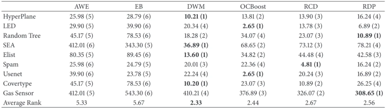
Figure 9: F1-measure on the Covertype.
CD 6 5 4 3 2 1 1.8889 RDP 2.7778 RCD 3.1111 DWM 4.1111 EB 4.4444 OCBoost 4.6667 AWE
Figure 10: A critical different diagram for all classifiers against each other.
Figure 9 shows the F1-measure changes on the Covertype. An interesting finding is that the curve of OCBoost suffered the most dramatic fluctuation. Apart from these, the F1 -measure of RDP and RCD is relatively stable on this dataset. RDP gained the best performance on this dataset. It is also indicates that the algorithm has superior adaptability to the real stream environment.
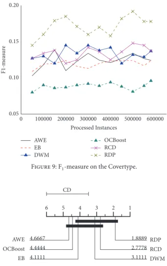
The average rank of classification accuracy of RDP on 9 synthetic and real-world data streams wins all other classifiers. To extend the analysis, nonparametric Friedman test was carried out for comparing multiple classifiers over multiple datasets [31]. The null hypothesis for the test is that there is no difference between the performances of all the tested algorithms. Moreover, in case of rejecting this null hypothesis, we employ the Nemenyi test [32] to verify whether the performance of our method is statistically different from the remaining algorithms. The critical differ-ence diagram shown in Figure 10 tells that our method is significantly better than AWE and OCBoost.
To summarize, RDP is superior to the other three from the following aspects: (1) It is capable of constructing a satisfactory model for handling both sudden and gradual concept drifts and has been specifically built to deal with
recurring concepts. (2)Compared to other ensembles, our method can achieve better performance and is robust against various noise levels and different types of drift.
5. Conclusion and Future Work
In this study, we focus on the investigation of Recurring Concept Drifts, a special subtype of concept drifts that has not yet drawn enough attention from the research community. A novel method intending to handle recurring concept based on the change detection method using classifier graph was proposed. The approach of detecting recurring drifts which allows reuse of previously learnt models enhanced the learn-ing performance on most datasets. Extensive experiments on synthetic and real-world datasets have validated that the proposed approach not only outperforms the existing popular methods in the adaptation to Recurring Concept Drifts, but also adapts well even in different concept drifting scenarios.
In our ongoing and future research, we will explore an effective procedure which will eliminate redundant classifiers without decreasing the ability to deal with recurring concepts and work toward developing classifier graph based effective practical dynamical learning mechanism.
Conflicts of Interest
The authors declare that they have no conflicts of interest.
Acknowledgments
This work was supported by the National Natural Sci-ence Foundation of China (no. 61672086, no. 61702030, no. 61771058, no. 61563001, and no. 61572005), the China Postdoctoral Science Foundation (2018M631328), the Natural Science Foundation of Beijing (no. 4182052), and Excellent Young Teachers Program of XYNU (no. 2016GGJS-08).
References
[1] C. C. Aggarwal,Data Streams: Models and Algorithms, Springer, Berlin, Germany, 2007.
[2] J. Gama,Knowledge Discovery from Data Streams, CRC Press, New Yourk, NY, USA, 2010.
[3] G. Widmer and M. Kubat, “Learning in the presence of concept drift and hidden contexts,”Machine Learning, vol. 23, no. 1, pp. 69–101, 1996.
[4] A. Tsymbal, “The problem of concept drift: Definitions and related work,” Tech. Rep., Department of Computer Science, Trinity College, Dublin, Ireland, 2004.
[5] G. Ditzler, M. Roveri, C. Alippi, and R. Polikar, “Learning in nonstationary environments: a survey,”IEEE Computational Intelligence Magazine, vol. 10, no. 4, pp. 12–25, 2015.
[6] G. Widmer, “Tracking Context Changes through Meta-Learn-ing,”Machine Learning, vol. 27, no. 3, pp. 259–286, 1997. [7] J. Gama, R. Sebasti˜ao, and P. P. Rodrigues, “Issues in evaluation
of stream learning algorithms,” inProceedings of the 15th ACM SIGKDD International Conference on Knowledge Discovery and
Data Mining (KDD ’09), pp. 329–338, ACM Press, New York, NY, USA, July 2009.
[8] I. Katakis, G. Tsoumakas, and I. Vlahavas, “Tracking recurring contexts using ensemble classifiers: an application to email filtering,”Knowledge and Information Systems, vol. 22, no. 3, pp. 371–391, 2010.
[9] J. Gama, I. ˇZliobait˙e, A. Bifet, M. Pechenizkiy, and A. Bouchachia, “A survey on concept drift adaptation,” ACM Computing Surveys, vol. 46, no. 4, pp. 231–238, 2014.
[10] R. Elwell and R. Polikar, “Incremental learning of concept drift in nonstationary environments,”IEEE Transactions on Neural Networks and Learning Systems, vol. 22, no. 10, pp. 1517–1531, 2011.
[11] J. Gama, P. Medas, G. Castillo, and P. Rodrigues, “Learning with drift detection,” inLearning with drift detection. In: Proceedings of the 17th Brazilian Symposium on Artificial Intelligence (SBIA 2004, LNCS 3171), Lecture Notes in Computer Science, pp. 286– 295, Springer, Berlin, Germany, 2004.
[12] M. Baena-Garc´ıa, D. J. Campo- ´Avila, R. Fidalgo et al., “Early drift detection method,” inProceedings of the Fourth Interna-tional Workshop on Knowledge Discovery from Data Streams (KDD 2006), pp. 77–86, ACM Press, New York, NY, USA, 2006. [13] A. Bifet and R. Gavalda, “Learning from time-changing data with adaptive windowing,” inProceedings of the 7th SIAM Inter-national Conference on Data Mining (SDM 2007), C. Apte, D. Skillicorn, B. Liu et al., Eds., pp. 443–448, SIAM, Philadelphia, PA, USA, 2007.
[14] G. J. Ross, N. M. Adams, D. K. Tasoulis, and D. J. Hand, “Exponentially weighted moving average charts for detecting concept drift,”Pattern Recognition Letters, vol. 33, no. 2, pp. 191– 198, 2012.
[15] R. Pears, S. Sakthithasan, and Y. S. Koh, “Detecting concept change in dynamic data streams,”Machine Learning, vol. 97, no. 3, pp. 259–293, 2014.
[16] W. N. Street and Y. S. Kim, “A streaming ensemble algorithm (SEA) for large-scale classification,” inProceedings of the 7th ACM SIGKDD International Conference on Knowledge Discov-ery and Data Mining (KDD ’01), pp. 377–382, ACM Press, New York, NY, USA, August 2001.
[17] H. Wang, W. Fan, P. S. Yu, and J. Han, “Mining concept-drifting data streams using ensemble classifiers,” inProceedings of 9th ACM SIGKDD International Conference on Knowledge Discovery and Data Mining (KDD 2003), pp. 226–235, ACM Press, New York, NY, USA, 2003.
[18] J. Z. Kolter and M. A. Maloof, “Dynamic weighted majority: an ensemble method for drifting concepts,”Journal of Machine Learning Research, vol. 8, pp. 2755–2790, 2007.
[19] R. Pelossof, M. Jones, I. Vovsha, and C. Rudin, “Online coordinate boosting,” in Proceedings of the 2009 IEEE 12th International Conference on Computer Vision Workshops, ICCV Workshops 2009, pp. 1354–1361, IEEE, New York, NY, USA, October 2009.
[20] L. L. Minku and X. Yao, “DDD: a new ensemble approach for dealing with concept drift,”IEEE Transactions on Knowledge and Data Engineering, vol. 24, no. 4, pp. 619–633, 2012. [21] J. B. Gomes, E. Menasalvas, P. A. Sousa et al., “Mining recurring
concepts in a dynamic feature space,”IEEE Transactions on Neural Networks and Learning Systems, vol. 25, no. 1, pp. 95–110, 2014.
[22] M. A. Abad, J. B. Gomes, and E. Menasalvas, “Predicting recurring concepts on data-streams by means of a meta-model and a fuzzy similarity function,”Expert Systems With Applications, vol. 46, pp. 87–105, 2016.
[23] P. M. Gonc¸alves and R. S. M. D. Barros, “RCD: A recurring concept drift framework,”Pattern Recognition Letters, vol. 34, no. 9, pp. 1018–1025, 2013.
[24] W. Hoeffding, “Probability inequalities for sums of bounded random variables,”Journal of the American Statistical Associa-tion, vol. 58, no. 301, pp. 13–30, 1963.
[25] H. Chernoff, “A measure of asymptotic efficiency for tests of a hypothesis based on the sum of observations,” Annals of Mathematical Statistics, vol. 23, no. 4, pp. 493–507, 1952. [26] T. Peel, S. Anthoine, and L. Ralaivola, “Empirical bernstein
inequalities for U-statistics,” inAdvances in Neural Information Processing Systems, pp. 1903–1911, 2010.
[27] J. J. Goeman and A. Solari, “Multiple hypothesis testing in genomics,”Statistics in Medicine, vol. 33, no. 11, pp. 1946–1978, 2014.
[28] Z. Sid´ak, “Rectangular confidence regions for the means of multivariate normal distributions,” Journal of the American Statistical Association, vol. 62, no. 318, pp. 626–633, 1967. [29] A. Bifet, G. Holmes, R. Kirkby, and B. Pfahringer, “Moa: Massive
online analysis,”Journal of Machine Learning Research, vol. 11, pp. 1601–1604, 2010.
[30] M. Lichman, “UCI Machine Learning Repository,” Irvine, CA: University of California, School of Information and Computer Science, http://archive.ics.uci.edu/ml.
[31] J. Demˇsar, “Statistical comparisons of classifiers over multiple data sets,”Journal of Machine Learning Research, vol. 7, pp. 1–30, 2006.
[32] N. Settouti, M. E. Bechar, and M. A. Chikh, “Statistical com-parisons of the top 10 algorithms in data mining for classi-fication task,”International Journal of Interactive Multimedia and Artificial Intelligence, Special Issue on Artificial Intelligence Underpinning, vol. 4, no. 1, pp. 46–51, 2016.
Computer Games Technology International Journal of Hindawi www.hindawi.com Volume 2018 Hindawi www.hindawi.com Journal of
Engineering
Volume 2018 Advances inFuzzy
Systems
Hindawi www.hindawi.com Volume 2018 International Journal of Reconfigurable Computing Hindawi www.hindawi.com Volume 2018 Hindawi www.hindawi.com Volume 2018Applied
Computational
Intelligence and Soft
Computing
Advances inArtificial
Intelligence
Hindawi www.hindawi.com Volume 2018 Hindawi www.hindawi.com Volume 2018Civil Engineering
Advances inHindawi
www.hindawi.com Volume 2018 Electrical and Computer Engineering Journal of Journal of Computer Networks and Communications Hindawi www.hindawi.com Volume 2018 Hindawi www.hindawi.com Volume 2018
Multimedia
International Journal ofBiomedical Imaging
Hindawi www.hindawi.com Volume 2018 Hindawi www.hindawi.com Volume 2018 Engineering Mathematics International Journal ofRobotics
Journal of Hindawiwww.hindawi.com Volume 2018 Hindawiwww.hindawi.com Volume 2018
Computational Intelligence and Neuroscience Hindawi www.hindawi.com Volume 2018 Mathematical Problems in Engineering Modelling & Simulation in Engineering Hindawi www.hindawi.com Volume 2018
Hindawi Publishing Corporation
http://www.hindawi.com Volume 2013 Hindawi www.hindawi.com