Short-term Forecasting Methods Based on the LEI Approach: The Case of the Czech Republic

RESEARCH AND POLICY NOTES 1

7

0

0

2

Vojtěch Benda and Luboš Růžička: Short-term Forecasting Methods Based on the LEI Approach: The Case of the Czech Republic

Short-term Forecasting Methods Based on the LEI Approach:

The Case of the Czech Republic

Vojt

ě

ch Benda

Luboš R

ů

ži

č

ka

The Research and Policy Notes of the Czech National Bank (CNB) are intended to disseminate the results of the CNB’s research projects as well as the other research activities of both the staff of the CNB and collaborating outside contributors, including invited speakers. The Notes aim to present topics related to strategic issues or specific aspects of monetary policy and financial stability in a less technical manner than the CNB Working Paper Series. The Notes are refereed internationally. The referee process is managed by the CNB Research Department. The Notes are circulated to stimulate discussion. The views expressed are those of the authors and do not necessarily reflect the official views of the CNB. Printed and distributed by the Czech National Bank. Available at http://www.cnb.cz.

Reviewed by: Filip Rozsypal

(Czech National Bank )

Gerhard

Ruenstler

(European Central Bank)

Petr

Zem

č

ík

(CERGE – EI, Prague)

Project Coordinator: Juraj Antal

© Czech National Bank, December 2007

Vojt

ě

ch Benda and Luboš R

ů

ži

č

ka

Short-term Forecasting Methods Based on the LEI Approach:

The Case of the Czech Republic

Vojtěch Benda and Luboš Růžička∗

Abstract

This paper is aimed at developing short-term forecasting methods based on the LEI (leading economic indicators) approach. We use a set of econometric models (PCA, SURE) that provide estimates of GDP growth for the Czech economy for a co-incident quarter and a few quarters ahead. These models exploit monthly or quarterly indicators such as business surveys, financial or labour market indicators, monetary aggregates, interest rates and spreads, etc. that become available before the release of data on GDP growth itself. Our tests show that the LEIs provide relatively accurate forecasts of GDP fluctuations in the short run.

JEL Codes: C53, E17, E37.

Keywords: Leading indicators, principal component analysis, seemingly unrelated

regression estimate.

∗_{Vojtěch Benda, ING Bank (e-mail: [email protected]);}

Luboš Růžička, Czech National Bank, Monetary and Statistics Department (e-mail: [email protected]). This work was supported by Czech National Bank Research Project No. E3/2005.

Motto: “The indicator that has a near-perfect record of performance during a business cycle, but whose behavior cannot be explained, will not command or warrant much attention, since faith depends on understanding. On the other hand, the indicator that is suggested by theoretical considerations but has not been tested or does not perform as theory predicts will not command much attention either, since faith depends on performance.”

Klein and Moore (1982, p. 2)

Nontechnical Summary

Forecasters around the world face the problem of relatively long delays in official quarterly GDP data estimates. This is also the case in the Czech Republic, where the Statistical Office publishes its first preliminary estimates around 70 days after the end of the relevant quarter. In periods of relatively volatile economic development, the delayed quarterly GDP estimates can sometimes be viewed as looking into a ‘rear-view mirror’, whereas policymakers need to get more information regarding the current state of the economy. The problem of quarterly data availability has led to the development of methods exploiting more timely indicators, published at higher frequencies, which can provide a preliminary estimate of GDP changes in advance, before the official estimates are published. The indicators that are supposed to carry information regarding GDP fluctuations comprise so-called ‘hard’ indicators (such as activity data, labour market statistics, monetary indicators, etc.) and ‘soft’ indicators, represented mainly by monthly and weekly sentiment surveys.

The initial forecasting methods – exploiting leading, coincident and lagged indicators – were aimed at indicating the probability of business-cycle turning points (peaks and troughs). Those methods are still widely used by several economic institutions. However, owing to relatively short Czech time series and hence a lack of significant turning points in the past, the application of such methods to Czech economic-cycle forecasting is limited. On the other hand, in recent decades, more sophisticated econometric methods have been developed to provide direct forecasts of desired reference time series (such as GDP, industrial production and price indexes). In our article, we tested the forecasting performance of two of the most widely used methods, namely Principal Component Analysis (PCA) and Seemingly Unrelated Regression Estimation (SURE). We estimated two models for Czech quarterly GDP forecasts using a wide range of accessible quarterly and monthly indicators. These methods provide estimates of GDP changes for the past quarter (which have not been officially published yet) and also for the next two consecutive quarters.

We suspect that such models based on leading and coincident economic indicators (among other forecasting tools) can provide useful information for assessing the current state of the economy in the short term and hence are probably supportive for policymakers.

1. Introduction

Accurate and timely information about the current state of real economic activity is an important requirement for the monetary policy-making process. In reality, however, delays in publication of the official statistics mean that the complete picture of economic developments within a particular period emerges only some time after that period has elapsed. It follows that there is a need for using forecasting methods that are able to minimize such delays.

Early indication of shocks and turning points cannot be achieved solely by theoretical macro models operating typically in the medium- or long-term horizons. As a result, the recognition of short-term forecasting tools is very important for the decision-making on monetary policy measures. These tools are not necessarily in contradiction to theoretical macro-models.1 In fact, the information obtained from short-term forecasting models is essential for determining the initial economic conditions for running the core model in the first phase of the macroeconomic forecasting process.

We introduce short-term forecasting methods based on the coincident and leading economic indicators (LEI) approaches and apply them on Czech data. The leading indicators analytical methods are based on monthly or quarterly economic indicator series and can be used for estimating the growth rate of GDP or other reference series, such as consumption, industrial production, exports, etc., in the current quarter and several quarters ahead. Developing and using such short-term forecasting tools should enable us to indicate important fluctuations in economic activity as soon as possible, with a potentially beneficial impact on the timing of monetary policy measures.

The rest of this paper is organized as follows: In Section 2, we summarize the experience with LEIs, as reflected in the literature, as well as the practical experience of numerous institutions involved in economic forecasting. Section 3 then discusses the indicator selection strategy. Furthermore, in this section we describe two econometric methods for quantitative prediction of Czech real GDP growth, namely Principal Component Analysis (PCA) and Seemingly Unrelated Regression Estimation (SURE). The estimation results are described in Section 4. In Section 5 we provide a comparison of their predictive power with a simple ARMA model. Section 6 provides our conclusions.

2. Literature Overview

The analytical concept based on the use of coincident, leading or lagging economic indicators for macroeconomic predictions was developed in the 1940s. The purpose of these forecasting methods was to provide early warning of cyclical turning points, that is, of sustained changes of direction in aggregate economic activity.

1 _{For example, the QPM macroeconomic model, which is used as a core forecasting instrument by the Czech}

2.1 Methodology

The first successful attempt to develop such methods was made at the National Bureau of Economic Research (NBER) by Mitchell and Burns (1938). These authors tested and finally identified twelve leading, coincident and lagging indicators (length of the working week, unemployment claims, new manufacturing orders, vendor performance, net business formation, equipment orders, building permits, change in inventories, sensitive materials and borrowing, stock prices and money supply) that were able to spot turning points in U.S. economic activity. The main assumption was that the business cycle is, in terms of repeating phases of economic growth and recessions, inevitable and more or less recurrent.2

The method of Mitchell and Burns (1938) was further developed by other authors, especially by Moore (1950, 1955), who constructed a synthetic variable – the composite leading indicator (CLI) – able to predict turning points, peaks and troughs of the U.S. economy. Methods based on the construction of the CLI are still maintained and used by several international as well as local economic institutions. Probably the most acknowledged approaches are those of the NBER3 _and the OECD4 _{(see the next section for a more detailed overview of institutions dealing} systematically with short-term forecasting methods).

Further research concerning LEI-based forecasting techniques has concentrated on the development of new indicators, more precise identification of business-cycle turning points, and hence the implementation of modern econometric methods of time-series analysis.

Neftci (1982) introduced an abstract, stochastically non-linear time-series model driven by a finite-state Markov process. Leading and coincident indicators were characterized as two time series, each having potentially three unobservable components: a trend, noise and a Markov process. The Markov process switches between two states, or, more specifically, between upswings and downswings of a business cycle. Using the model, Neftci showed that the index of leading indicators may provide a consistent estimate of the present state of the Markov process. Palash and Radecki (1985) successfully tested Neftci’s claim using the CLI constructed by the U.S. Department of Commerce to signal a recession when the cumulative downturn probability rises above 90 per cent. Another successful application of Neftci’s method to international data (the USA, Japan, the United Kingdom and West Germany) was that of Niemira (1993).

All the methods mentioned above represent the first group of forecasting techniques using the LEI approach. They are similar concerning their emphasis on qualitative anticipation of business-cycle turning points. They do not usually command satisfactory (if any) information about the accurate timing of those turning points, the size of the cyclical expansions or contractions and the length of

2 _{Burns and Mitchell (1946) defined the business cycle as follows: “Business cycles are a type of fluctuation}

found in the aggregate economic activity of nations that organize their work mainly in business enterprises: a cycle consists of expansions occurring at about the same time in many economic activities, followed by similarly general recessions, contractions and revivals, that merge into the expansion phase of the next cycle; this sequence of changes is recurrent but not periodic. In duration business cycles vary from more than a year to ten or twelve years; they are not divisible into shorter cycles of similar character with amplitudes approximating their own.”

3 _{See Zarnowitz (1973, 1982) or Vaccara (1978).}

4 _{For further details concerning the OECD methodology for constructing the CLI see}

particular cyclical phases. To sum up, they do not provide any information on GDP, or any other variable linked to the business cycle, apart from the cyclical turning points.

The second group of forecasting techniques based on LEIs differs from the methods mentioned above in terms of their emphasis on the use of more sophisticated econometric methods and their focus on direct – quantitative – forecasting of observable time series (such as GDP, inflation, unemployment, etc.) or latent variables (such as the output gap). Unlike the methods that give the greatest weight to the anticipation of cyclical turning points, the same importance is given to each observation of the reference time series. Further assessment of the current state of the business cycle, and hence the likelihood of recession or expansion, can be extracted from the projection of reference series (e.g. GDP) on some periods ahead by selected means of transformation (such as the Kalman filter).

For quantitative forecasts, a large variety of econometric methods is used. The most frequently used are the following: the single-index model of Stock and Watson, Principal Component Analysis (PCA) and Seemingly Unrelated Regression Estimation (SURE).

A direct quantitative forecast of a latent variable representing the business cycle is provided, for example, by the single-index model method developed by Stock and Watson (1989, 1991). Instead of observable variables such as GDP or employment, Stock and Watson estimate an unobservable index5 _{that is common to multiple macroeconomic variables. Estimate of this} unobserved index, which consists of variables that move contemporaneously with this index, provides an alternative index of coincident indicators. This index can then be forecasted using the leading variables. This method was exploited by BEA6 _{for forecasting the business cycle of the} U.S. economy. The failure of the model to anticipate the 1990 recession reduced its credibility and the BEA no longer publishes this index (Salazar, 1996).

An approach that can use numerous LEIs for estimation of reference time series is Principal Component Analysis (PCA). This method allows the information contained in many mutually correlated variables, i.e. leading and coincident indicators, to be transformed into a small number of vectors (principal components). These orthogonal vectors are supposed to explain a substantial part of the information contained in the group of variables initially selected. The principal components are subsequently used for estimation of the reference time series (for details of the PCA methodology see Section 3).

There is relatively large number of recent studies exploiting this method for short-term forecasts. One example is Angelini et al. (2001), who explored this method for the euro area using a multi-country data set and a broad array of variables in order to test the inflation performance of extracted factors at the aggregate euro area level.

5 _{Stock And Watson (1996) preferred the unobservable index to observable variables (such as GDP or}

employment) since “…these series measure only various facets of the overall state of the economic activity; none measure the state of the economy [in Burns and Mitchell’s (1946) terminology, the ‘reference cycle’] directly”.

In addition, Artus et. al. (1996) constructed a PCA-based leading indicator that can be used to estimate the growth rate of French GDP in the current and coming quarter. This indicator is an optimal combination of factors calculated from basic series (including both “soft” and “hard” indicators), and those factors can be interpreted from an economic viewpoint.

Furthermore, Stock and Watson (2002), in their article, study the forecasting of U.S. macroeconomic time series variables using a large number of predictors. They forecast eight variables, four of which are the measures of real economic activity used to construct the Index of Coincident Economic Indicators maintained by the Conference Board7 _{(formerly by the U.S.} Department of Commerce): industrial production; real personal income less transfers; real manufacturing and trade sales; and number of employees on non-agricultural payrolls. The remaining four series are price indexes: the consumer price index (CPI); the personal consumption expenditure implicit price deflator (PCE); the CPI less food and energy; and the producer price index for finished goods. The predictors are summarized using a small number of indexes constructed by PCA. An approximate dynamic factor model serves as the statistical framework for the estimation of the indexes and construction of the forecasts. The method is used to construct 6-, 12-, and 24-month-ahead forecasts for eight monthly U.S. macroeconomic time series using 215 predictors in simulated real time from 1970 through 1998. During this sample period these new forecasts outperformed univariate autoregressions, small vector autoregressions and leading indicator models.

Moreover, Sédillot and Pain (2003) developed a set of econometric models using PCA that provide estimates of GDP growth for a number of major OECD countries and zones in the two quarters following the last quarter for which official data have been published. These models exploit the amount of monthly conjunctural information that becomes available before the release of official national data. Information is incorporated from both “soft” indicators, such as business surveys, and “hard” indicators, such as industrial production and retail sales. High frequency indicators are recast into quarterly GDP figures using univariate or multivariate “bridge” models. Among the other studies exploiting the PCA method, we can also mention the approach of Schumacher (2005) to the estimation of German quarterly GDP growth, and that of Pula and Reiff (2002), who provide a factor model for estimation of short-term industrial growth in Hungary using information taken from Hungarian business survey indicators.

Another short-term forecasting technique using the LEI approach is based on a system of four equations estimating q-o-q changes in GDP. Each equation explains GDP growth in a subsequent quarter. Therefore, the system enables us to estimate GDP growth in the coincident quarter and three quarters ahead. For the estimation of the parameters of the system the Seemingly Unrelated Regression Estimation8 _{(SURE) method is used.}

7 _{The Conference Board (TCB) is a worldwide business and research organization producing, for example,}

confidence indexes and leading economic indicators. It connects nearly 2,000 companies in 60 countries. TCB is quoted more than 34,500 times a year in the media, making it the world’s most widely quoted private source of economic information. For further details concerning the Conference Board and its CLI methodology, see http://www.conference-board.org/economics/bci/.

8 _{This method was first introduced by Zellner (1962). That is why it is sometimes referred to as “Zellner´s}

This method estimates the parameters of the system, accounting for heteroscedasticity and contemporaneous correlation in the errors across equations. This aspect is essential, since the individual equations of the system are interlinked through the residuals (for more information about the SURE methodology see Section 3). A practical example of the use of this method for LEI-based forecasting of GDP in the UK is provided by Salazar, Smith and Weale (1996).

2.2 Institutions

The OECD regularly publishes a CLI based on several (usually five) indicators for its member countries. The most frequently used indicators for constructing the CLI are the following: new orders in manufacturing, M1 money supply, the yield on public-sector bonds, share prices, unit labour costs, and the spread of interest rates.9 _{The business cycle is represented by trend-adjusted} industrial production.10

A similar approach is used, for example, by The Conference Board (TCB), although with some differences in technical terms. The Central Planning Bureau of the Netherlands uses a more disaggregated system.11 _{This institution produces LEI-based forecasts not only for GDP, but also} for other GDP components (such as private consumption, investment and exports). Subsequently, the predictions of those particular components are implemented into the so-called FKSEC quarterly macroeconomic model for the Netherlands (Kroese, 1992).

In addition, a CLI for eleven countries is supplied by the Center for International Business Cycle Research (CIBCR) at the Columbia University Business School. For the U.S. economy, a CLI construction is also provided by the U.S. Department of Commerce (DOC). For the Czech economy, the Ministry of Finance publishes a composite leading indicator in its quarterly macroeconomic prediction.12 _{The CLI construction methodology can be used not only for the} prediction of business-cycle turning points, but also for the prediction of price index turning points (e.g. for consumer or housing prices), as in the case of the BEA.

2.3 Criticism and Limitations

Since the main purpose of this paper is to apply the LEI-based forecasting methods suitable for more precise forecasting of Czech GDP in the short term, and hence the current state of business cycle, we have to evaluate carefully the usefulness of all the techniques mentioned in this section. There is one general stream of criticism, expressed, for example, by Koopmans (1947) with regard to the NBER methodology. The main argument is that it does not provide an adequate theoretical background for the use of particular leading indicators as predictors of business-cycle turning points. Furthermore, it is strictly based on statistical regularities and does not lead to inferences about stabilization policies.

9 _{For each OECD country the CLI is composed of a different set of indicators according to their ability to predict}

turning points. For the full list of indicators for particular countries, see http://www.oecd.org.

10 _{The trend adjustment is carried out by a technique called the phase average trend (PAT) method. See}

Zarnowitz (2002).

11 _{See Kranendonk (1997).}

As also noted by Salazar, Smith and Weale (1996, p.1), “…theories of business cycles based both on the notion of monetary policy surprises, or the more recent Real Business Cycle theory driven by technological shocks, both imply that cycles – however defined – are inherently unpredictable”. In addition, the CLI-based methods require relatively long time series with a sufficient number of turning points (peaks and troughs), which prevents their use on shorter time series.

Apart from the theoretical objections mentioned above, there is also another complication associated with the limited length of the Czech GDP time series. It starts from 1995 and shows only four turning points (two peaks and two troughs), a number we find insufficient for applying the qualitative methods for turning-point forecasting. Moreover, if we want to approximate the Czech business cycle by industrial production on a monthly basis (which corresponds with the OECD or NBER techniques), we come across a problem with insignificant correlation between industrial production and GDP (see Figure 1 in the Appendix). This is probably due to the rapid structural changes observed in the industrial sector in the past decade. Also, this finding complicates the adoption of qualitative techniques in the Czech case.

As a result, all methods for assessing cyclical turning points qualitatively (including the single-index model by Stock and Watson) seem inappropriate in the Czech case. On the contrary, quantitative methods such as PCA and SURE, exploiting all accessible statistical observations, appear more suitable in the Czech case.

Based on this critical overview, we decided to conduct a GDP forecast for the Czech Republic based on the PCA method. In addition, we explore another technique based on a system of four regression equations using the SURE method.

3. Estimation Methodology

The appropriate methodology for short-term forecasting has to cope not only with the choice of appropriate technical means, but also with the selection of suitable indicators. That is why, before introducing our methodology in technical terms, we find it useful to discuss briefly the indicator selection strategy.

3.1 Indicator Selection Strategy

During the process of selection and classification of leading economic indicators suitable for short-term forecasting, the empirical evidence and economic theory interact closely – see Klein and More (1982) for a precise formulation of basic rules for the indicator selection strategy. In other words, the leading indicators chosen should be intuitive enough in terms of theoretical economic reasoning, but at the same time we have to be aware whether – apart from satisfactory statistical tests – they also provide interpretable leads and their coefficients have acceptable signs. With regard to economic reasoning, the LEIs can be classified as follows13_{: (i) prime movers, i.e.} indicators explaining fluctuations in economic activity that are driven basically by new measurable forces (monetary and fiscal policy); (ii) assessment of actual situation and market expectations, meaning that some time series (such as business surveys, confidence indicators, etc.)

are more sensitive to expectations about future economic activity; and finally (iii) early-stage signals of economic activity, i.e. indicators signalling that changes in economic activity are on the way (unemployment/vacancy ratio, order books, inventory stock, etc.).

In addition, the fluctuation of the chosen LEIs should display a high correlation with GDP. That is why the accessibility of data sources is an important requirement. LEIs should be accessible in advance of the release of GDP figures and must not “suffer” from frequent revisions. Higher frequency (quarterly or monthly) is obviously an advantage.

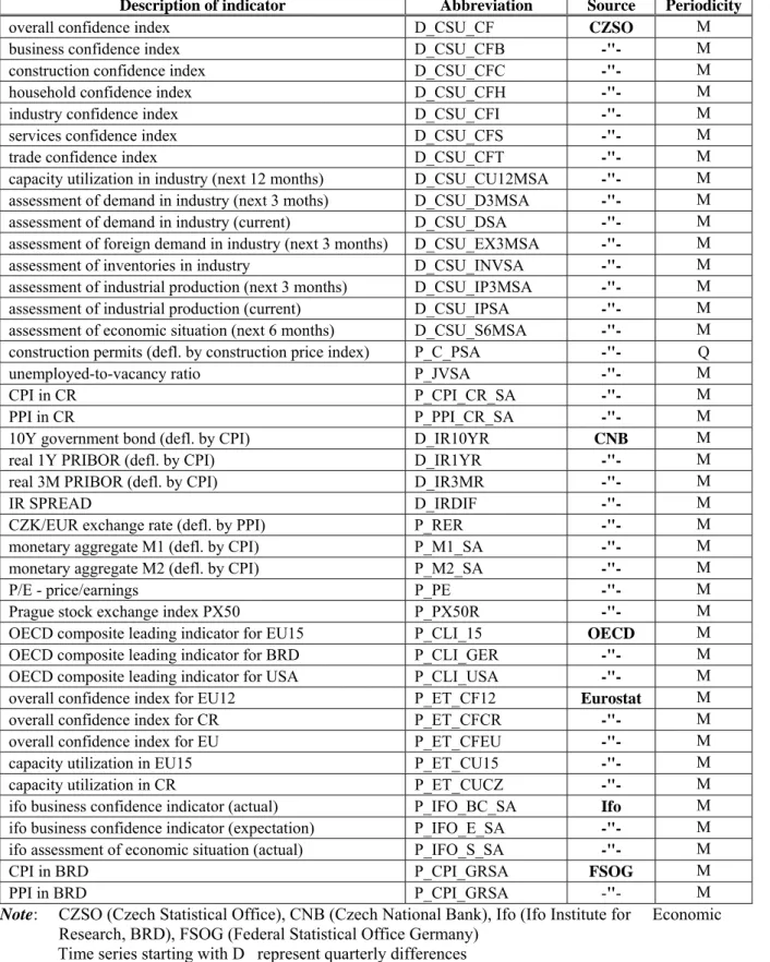
For the present paper, we chose a range of various leading indicators that fulfil the requirements defined above. The so-called prime movers include indicators such as interest rates, the exchange rate and monetary aggregates. Assessment of the actual situation underlies the indicators from CZSO business surveys, the leading indicators of the OECD and IFO-Institute, and stock-exchange indicators. And finally, early-stage signals of economic activity comprise indicators from the labour-force statistics (unemployed-to-vacancy ratio), construction permits and expected capacity utilization. According to the available indicators, the biggest group comprises indicators from CZSO business surveys (assessment of the actual situation). The complete list of 41 gathered and tested leading economic indicators is given in Table 1 in the Appendix.

Preliminary quarterly GDP data are often subject to large and repeated revisions until they are harmonized with the annual national accounts.14 _{This is why we decided to omit the recent GDP} figures (2006Q1–2007Q2).

3.2 Principal Component Analysis Methodology

We have numerous groups of leading indicators, which have various levels of correlation with the reference time series (GDP in our case) and also among themselves. If we try to estimate the reference time series as a linear combination of leading indicators, in some cases the correlation between two or more indicators could be fairly high and then we have to cope with the problem of multicollinearity.

There are several methods for dealing with multicollinearity. The easiest (and probably the most frequently used) is to drop the variables suspected of causing the problem from the regression equation. The disadvantage of using this method relates to the problem of specification and loss of information (due to the low number of observations we would have to drop too many variables – probably more than half of the total).

One way of handling the multicollinearity problem is to employ principal component analysis. In the case of substantial collinearity among the vectors of the data matrix (in our case among the leading indicators), there exist only a limited number of independent sources of variation. Principal component analysis is used in an attempt to extract from the data matrix (a large set of mutually correlated time series) a small number of independent variables (called principal components) which account for a substantial part of the total variation in the data matrix.

Algebraically, we may approach the calculation of principal components as a regression problem. We need to find such vectors z, calculated as the linear combination of the columns of matrixX, which provide the best fit to all of the columns of X (we consider now that the data matrix has

Kcolumns which may have fewer than Kindependent sources of variation). The linear combination will be:

.

Xc

z

=

(1)

The uniqueness of the vector z is guaranteed by imposing:

.

1

'

_z

₌

z

(2)

If we consider only one columnx_k of matrix X and regress the column on the newly constructed vector, the sum of squared residuals from the regression will be

.

]

[

]

)

(

[

' 1 ' ' ' ' ' k k k k k k

e

x

I

z

z

z

z

x

x

I

zz

x

e

=

−

−

=

−

(3) If we consider all the columnsx_ksof matrixX simultaneously, we seek to minimize

),

]

[

(

' ' '

_e

_tr

_X

_I

_zz

_X

e

k k k

=

−

∑

(4) subject to

z

'

z

=

1

. This is the same as maximizing the second part of the trace, since the first part does not involve c. The maximum value of the second part of (4) is achieved for cequal to the characteristic vector associated with the largest characteristic root.

If the total variation in X is defined as the trace of X'X_{, the proportion of the variation in} X

X' _{explained by this variable is}

,

1 1 1

∑

=

=

_K k k

w

λ

λ

(5)

where λ denotes the characteristic root andλ₁ is the largest. The above procedure can be repeated. We need to find a second linear combination of the columns of X with the same criterion, subject to the condition that this second variable must be orthogonal to the first. Altogether there are K variables (principal components); the t-th is computed using the characteristic vector corresponding the t-th largest characteristic root. If we use allKprincipal components, we end up exactly where we started.

The point of the previous exercise is to use a smaller number of principal componentsL<K, so that their contribution to the explanation of the total variation is satisfactorily close to one. The decision regarding how many components to retain could be an arbitrary one, but there are some guidelines (criteria) that are used in practice. For our purposes, we decide to use the Kaiser criterion, which suggests retaining only those components associated with a characteristic root greater than 1. This criterion says that unless a component extracts at least as much as the equivalent of one original variable, we drop it. The characteristic roots are presented together with the explained proportion of the total variability in Table 2 in the Appendix.

Finally, instead of the initial matrixX we use matrixXC_L, whereC_Lis a K×Lmatrix containing

Lcharacteristic vectors ofX'X _{. Matrix}

L

XC containsLprincipal components, which are used as explanatory variables in the regression for the estimation of the reference time series (GDP).

3.3 Seemingly Unrelated Regression Estimation (SURE) Methodology

The methodology is based on the assumption that a future change in GDP is indicated in advance by changes in several leading indicators (for example a change in the number of construction permits indicates a change in activity in construction and consequently a change in GDP). SURE enables us to conduct forecasts not only for the coincident quarter, but also for several quarters ahead. This is possible due to the presence of an appropriate number of LEIs that can explain fluctuations in the reference time series not only in the present quarter, but also in the following quarters (a satisfactorily long lag between cause and effect). It is natural that the further we go into the future, the lower is the explanatory power.

SURE enables us to estimate equations for predicting GDP growth and to avoid the problems mentioned in Salazar, Smith and Weale (1996).15

This method assumes that the quarterly change in output (y) one quarter ahead has an underlying dynamic relationship with a vector of indicator variables (x) which can be represented in the following way: t t t t t t

x

x

x

L

x

u

y

+1

=

α

'

+

β

'

−1

+

γ

'

− 2

+

δ

'

(

)

−3

+

(6)

The vector of coefficients α, β and γ picks out those variables which are “shorter leading indicators”, at lags 1, 2 and 3, while the vector lag polynomial δ’(L) picks out those which are “longer leading indicators”. We assume that the error term is white noise and x can be presented in the following vector autoregressive form:

t t

t L x v

x +1= Φ ( ) + , (7)

where Φ(L)=

φ

0+

φ

1L+

φ

2L+.... Then, using recursive substitution, the quarterly change in

output (two, three and four quarters ahead) can be expressed as:

, )) ( ' ) ( ' ( ) ' ' ( ) ' ' ( 0 1 1 2 2 2 2 t t t t t x x L L x e y + = Ψ +

β

+ Ψ +

γ

− + Ψ +

δ

− + (8)

,

))

(

'

)

(

'

(

)

'

'

(

0 1 1 3 3 t t t t

x

L

L

x

e

y

+

=

Θ

+

γ

+

Θ

+

δ

−

+

(9)

.

))

(

'

)

(

'

(

4 4 t t t

L

L

x

e

y

+

=

Γ

+

δ

+

, (10)

where Ψi,Θi and Γi are functions of the coefficients

φ

i,

α

,

β

and

γ

, and eit include a moving average element (e_itare a function of lags of vt). In our SURE estimation (in an unrestricted form), a system of four equations is estimated, with the structure given above.

It is worth mentioning that the left-hand side variables are q-o-q changes in output shifted one quarter ahead. The right-hand side of the equations contains only the different leading indicators with various lags. The leading indicators are linked by the system of serial correlations. According to equation (7), the vector of the leading indicators x is represented by the vector autoregressive form. Many elements of Ψi,Θi and Γi turned out to be highly insignificant (

α

,

β

and

γ

are sparse and there is little system persistence inΦ(L)). By setting these elements to zero, SURE

estimation improves the efficiency of the estimation by pooling the estimation of many elements in α, β, γ and δ’(L) across all four equations. This implies that the set of variables appearing in equation (8) is a subset of those appearing in equation (6) and so forth.

4. Results

In this section, we summarise our results based on the methodologies described above. First, we present the results obtained from the Principal Component Analysis (PCA). Subsequently, the results of the Seemingly Unrelated Regression Estimation (SURE) method are also presented.

4.1 PCA Results

Initially, we collected 41 leading indicators (see Table 1 in the Appendix). However, not all of them are suitable for our analytical purposes, primarily due to their shortness (the confidence index of households, the confidence index of services and the 10-year interest rate on government bonds started to be published after 2000). Even after subtracting the aforementioned indicators unsuitable for PCA, we still had a high number of variables and only a limited number of observations (only 37 considering the maximum possible sample 1996Q2–2005Q4). To maintain the required number of degrees of freedom we had to make a further reduction in the number of variables as explained below.

The second reduction in the number of variables was made by correlation analysis. Some leading indicators were very closely correlated, or gave approximately the same information, so it was not reasonable to use all of them. For example, the Eurostat indicator for the EU-12 and the Eurostat indicator for the EU as a whole had a correlation coefficient of r = 0.98. Similarly high correlation coefficients were detected in the case of the indicators evaluating the situation in industry at present and after 3 months. The same applied to the evaluation of demand, the OECD Composite Leading Index for the EU-15 and Germany, the IFO Industry Index and the IFO Industry Outlook. In this way we reduced the total number of leading indicators used as PCA inputs to a total of 30. Some published time series were already seasonally adjusted, but some were not. Those series which a contained statistically significant seasonal component were adjusted by CENSUS X-11 ARIMA. Afterwards, the leading indicators were transformed into quarterly percentage changes (data with monthly periodicity were averaged into quarterly and also transformed into q-o-q changes) and tested for stationarity.

Only the time series of real GDP appears to be nonstationary. One cause of the nonstationarity is considerable fluctuation in the q-o-q changes in 1996–1998 (changes in methodology, a monetary crisis). To eliminate the problems that these considerable fluctuations could cause, we decided to omit this early period and start the sample in the first quarter of 1999. Nevertheless, after the reduction this time series stays constantly nonstationary (a constant acceleration in q-o-q GDP growth since the beginning of 2002). Although we realised that the nonstationarity of the time series could cause problems in our later computations, we decided to work with this series and try to construct linear regression models. The situation was very similar in the case of y-o-y changes in GDP.

In order to retain the number of degrees of freedom needed for the estimation, the reduction of the sample required a further reduction in the number of leading indicators. This reduction was based on our empirical knowledge only. We weighed up the relevance of particular indicators with regard to GDP and omitted the least relevant indicators from the analysis. So, the final number of variables used for PCA was 23, as listed in Table 3 in the Appendix.

From these 23 leading indicators we computed the principal components, and based on Kaiser’s criterion we decided to choose the first eight explaining nearly 82% of the total variability of the 23 leading indicators used (see Table 2 in the Appendix).

In the following stage of our work we tried to find an appropriate economic interpretation for these eight synthetic variables (principal components – PCs). To do so, we considered the correlations between particular components and the basic leading indicators. The results of this analysis are summarized in Table 4. Signs +/- evaluate the different intensity of the correlation. In the following part we specify some interpretation of the eight principal components.

PC 1 is positively correlated with the domestic demand indicators (overall demand index,

business confidence index, industry confidence index) and also with the foreign demand indicators (foreign demand index, OECD leading index of Germany and USA, Eurostat confidence index of EU-12). We can thus interpret the first PC as a substitute for the demand variables.

PC 2 is highly negatively correlated with the unemployed-to-vacancy ratio. So, this component

evaluates the situation on the labour market.

PC 3, PC 4 and PC 5 are linked to construction permits, domestic and foreign industrial

production, the trade confidence index, foreign inflation, the exchange rate and inventories (with different signs) and in these cases it is very difficult to find an adequate interpretation for these PCs.

PC 6, PC 7 and PC8 are positively correlated with the Prague stock exchange index and the

domestic interest rate.

To illustrate the economic interpretation of the principal components, we also constructed charts 2 and 3, which show the chronological changes of the principal components and the most important indicators (highly correlated with the PCs).

4.2 Relation between Real GDP Growth and PCs

We tried to construct single econometric models linking q-o-q real growth of GDP to the principal components computed by PCA. All the computed principal components could be used as explanatory variables in the regression equations, but the higher is the number of the component, the lower is its explanatory power. In our case, the components from eight onwards turned out to be insignificant and hence were excluded from the regression.

It is also important to take into account the position of the month in which the forecast is made within the quarter. The GDP data are published quarterly (with a lag of approximately 70 days after the end of the quarter), whereas the majority of the leading indicators are published monthly. The more months of the quarter have passed, the more information from the leading indicators we

can exploit so as to forecast GDP changes. For example, if we make a forecast using the information of the first two months of the current quarter, we need to estimate GDP growth in the past quarter (which has not been published yet). We can also estimate the current quarter, because we already have some information about it. We can also make a forecast for the quarter ahead, because we believe that there is a lag between changes in the leading indicators and changes in GDP. In the third month of the current quarter, we can estimate only the current quarter (nearly all the information is available) and the quarter ahead. So, we present two regression models. The first one estimates the GDP change in the previous and current quarters, while the second is used for estimation of the quarter ahead.

The following section presents detailed results of the regression models estimating GDP growth from the principal components.

Estimation for the Previous and Current Quarters:

HDP_QOQ = 0.1188 + 0.001960*PC1 - 0.007230*PC2 - 0.013082*PC6 + 0.027314*PC8 + (0.0808) (0.0015) (0.0034) (0.0084) (0.0098) (1.4698) (1.3116) (-2.1016) (-1.5645) (2.7710) + 0.940364*HDP_QOQ(-1) (0.0832) (11.296)

In brackets below the value of the coefficient is the standard error of the coefficient followed by the t-statistic.

R2 adj.= 0.85 F-stat = 31.82 S.E. of regression = 0.17 Jarque-Bera statistic = 1.28 Autocorrelation of the residuals was tested for using the Ljung-Box test and the LM test – there is no autocorrelation up to lag 12.

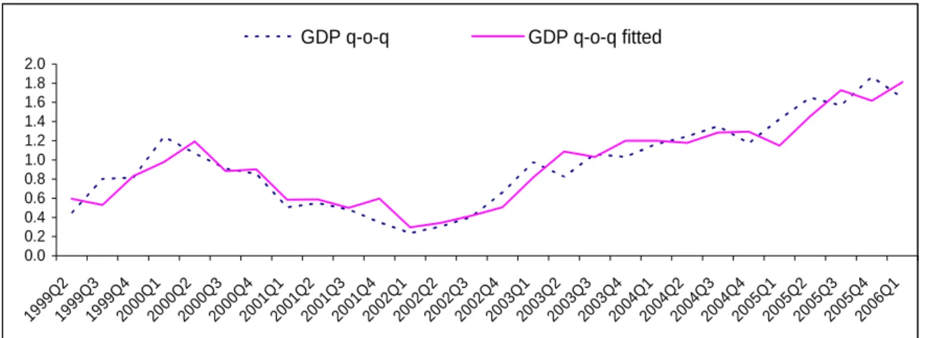
Figure 1: Real GDP and the Fit of the Model

0.0 0.2 0.4 0.6 0.8 1.0 1.2 1.4 1.6 1.8 2.0 1999Q 2 1999Q 3 1999Q 4 2000Q 1 2000 Q2 2000Q 3 2000Q 4 2001Q 1 2001Q 2 2001Q 3 2001Q 4 2002 Q1 2002Q 2 2002Q 3 2002Q 4 2003Q 1 2003Q 2 2003Q 3 2003 Q4 2004Q 1 2004Q 2 2004Q 3 2004Q 4 2005Q 1 2005Q 2 2005 Q3 2005Q 4 2006Q 1

Estimation for a Quarter Ahead:

HDP_QOQ(+1) = 0.138 + 0.003097*PC1 - 0.008017*PC2 + 0.02972*PC8 + 0.953008*HDP_QOQ(-1)

(0.0968) (0.0017) (0.0040) (0.0084) (0.1051) (1.4250) (1.7901) (-1.9837) (3.5060) (9.0657)

R2 _{adj.= 0.78 F-stat = 24.39 S.E. of regression = 0.21 Jarque-Bera statistic = 0.78} Autocorrelation of the residuals was tested for using the Ljung-Box test and the LM test – there is no autocorrelation up to lag 12.

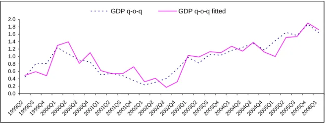
Figure 2: Real GDP and the Fit of the Model

0.0 0.2 0.4 0.6 0.8 1.0 1.2 1.4 1.6 1.8 2.0 1999Q 2 1999Q 3 1999 Q4 2000Q 1 2000Q 2 2000Q 3 2000 Q4 2001Q 1 2001Q 2 2001Q 3 2001Q 4 2002Q 1 2002Q 2 2002Q 3 2002Q 4 2003 Q1 2003Q 2 2003Q 3 2003Q 4 2004Q 1 2004Q 2 2004Q 3 2004Q 4 2005Q 1 2005 Q2 2005Q 3 2005Q 4 2006Q 1

GDP q-o-q GDP q-o-q fitted

The parameters of the presented models demonstrate that their estimated power is quite satisfactory (the adjusted coefficients of determination of both models are very high). The quality of the models is confirmed by figures 1 and 2. Both models contain a lagged dependent variable. This fact is not very plausible (the estimated parameter is too close to one, causing problems with forecasting), but the addition of this variable was necessary for elimination of the first order of autocorrelation of the residuals. As soon as a longer GDP time series is available, the trend of constant acceleration of GDP is likely to fade away, the series of q-o-q changes are likely to be stationary and the problems with autocorrelation of the residuals presumably disappear. There is also the possibility of considering lagged GDP as one of the leading indicators. But incorporating GDP into the group of indicators entering the PCA does not eliminate the problem of serially correlated residuals in the regression equations.

We also tried to construct a model for estimating y-o-y changes in GDP where the principal components were also used as the explanatory variables. In this case, the final outcome was very unsatisfactory (permanent presence of autocorrelation of the residuals).

4.3 SURE Results

The same transformations and tests as in the case of the PCA were performed before the estimation of the SUR system (seasonal time series were seasonally adjusted, and all were transformed into q-o-q changes and tested for stationarity).

After that, the relation between each particular LEI and GDP growth was tested with the Granger causality test and the cross-correlation method (using a fairly lax significance criterion). For the

results of the cross correlations, see table 4. Afterwards, the potential LEIs with the best performance and most significant lags were added into the regressions for each estimate – for the coincident quarter and one, two and three quarters ahead with respect to the cross-equation restriction. This means that if a variable enters the equation for the coincident quarter with a lag of four quarters (relative to the current quarter), it enters the equation for three quarters ahead with a lag of one quarter.

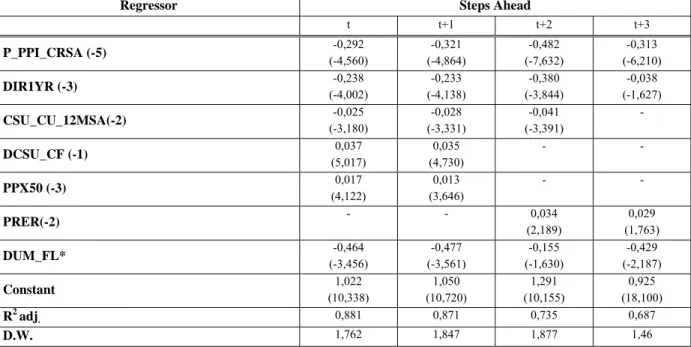
Each equation for the particular quarters was estimated separately using the OLS approach. Furthermore, the regressors with an insignificant p-value and/or an inappropriate sign were rejected. Finally, all four equations were estimated as a system using the SURE approach. For the estimate we used the sample covering the period 1998Q1–2005Q4, since several indicators, such as capacity utilization, were not published before that date. The estimation results are described in Table 5 in the Appendix. The numbers in parenthesis identify the lags used in the equation for the coincident quarter (t).

For consecutive equations, the number of lags declines stepwise. For each variable, the table shows the values of the estimated coefficients and t-statistics (in parenthesis). SURE provides satisfactory estimates of GDP growth for the coincident quarter and one quarter ahead, in terms of adjusted R2 _{values of 0.87 for both equations. The explanatory power of the equations for Q(t+2)} and Q(t+3) is less satisfying, partly due to the lower number of explanatory variables.16 Nevertheless, the equations for the last two quarters ahead provide useful information in terms of an early warning signal concerning changes in the pace of GDP growth.

The theoretical reasoning behind the chosen variables, no matter how intuitive it is, can be described as follows. The industrial price index (P_PPI_CRSA) comprises a supply-side cost shock, which is likely to affect the market competitiveness of industrial producers and hence their economic performance. Interest rates (DIR1YR) represent one of the crucial factors of the investment and consumption decision-making process. Positive changes in real interest rates are likely to negatively affect business capital formation and/or private consumption and hence also GDP growth. Capacity utilization (CSU_CU_12MSA) can serve as a proxy for the stage in the business cycle. The higher is the capacity utilization of the economy, the more likely is an economic slowdown following an economic overheating. The confidence indicator (DCSU_CF) represents typical prime-mover-like economic indicators. The investment or consumer decision-making in the short term is usually very dependent on how the investor and/or consumer evaluate the potential for economic growth. The equity index (PPX50) embraces the market’s evaluation of the economic stance and the future performance of businesses traded on the stock exchange. An increase in the real exchange rate (PRER) (in the sense of depreciation) represents a positive factor for economic growth, as it supports the competitiveness of domestic export-oriented businesses and hence export growth. Finally, the dummy variable represents the temporary distorting effects of floods on economic performance.

16 _{Compared to the equations for Q(t) and Q(t+1), two explanatory indicators (the overall confidence index and}

5. Comparison with Simple ARMA Model

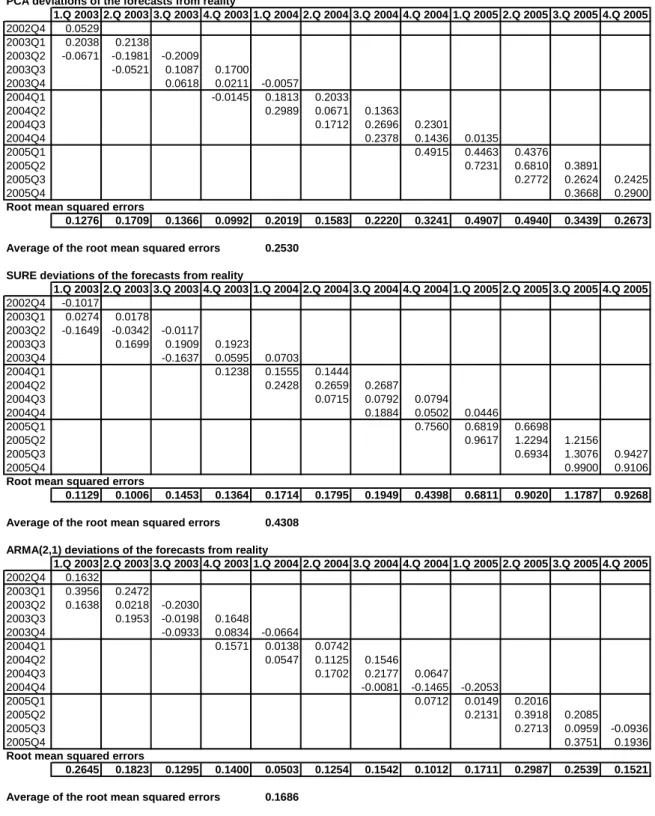
In order to evaluate the accuracy of the PCA and SURE forecasts of GDP, we decided to compare them with the forecasts derived from a simple ARMA(2,1) model. Since PCA and SURE are short-term forecasting methods for several subsequent quarters, the predictive interval was set at three quarters. We measured the deviations of the particular in-sample forecasts from the actual fluctuations in real GDP. The first forecast was made for the first quarter of 2003 and the last for the fourth quarter of 2005 (altogether 12 forecasts). We were not able to compute out-of-sample forecasts because of a shortage of data (due to the reduced number of observations we ran out of degrees of freedom and hence could not compute the factors from PCA). From the deviations we computed the root mean squared errors for each forecast and finally the average of these root mean squared errors for each method.

The results of our analysis are summarized in Table 6. According to the values of the root mean squared errors, the best forecasting performance is given by the simple ARMA(2,1) model. This might indicate that the construction of the more sophisticated PCA and SURE methods is pointless. But it is worth mentioning that the q-o-q GDP growth in the tested period from 2003Q1–2005Q4 was steadily accelerating. The ARMA forecasts kept the trend of the real data and that is why this simple model had the lowest forecast errors. On the other hand, the methods based on leading and coincident indicators were influenced by the fact that neither the short-term indicators (monthly data) nor the data from polls of sentiment suggest such buoyant growth. As soon as the change in GDP growth starts to moderate, the ARMA model forecasts will probably follow the growth trend and hence the accuracy of the ARMA model will drop rapidly, while the methods based on leading and coincident indicators will probably have better performance during the period of trend change. From the tables it is apparent that the root mean squared errors of all three methods during the first half of the examined period are comparable. In the second half of the period, the ARMA errors remained almost the same but the PCA and SURE errors increased significantly (the indicators did not expect q-o-q GDP growth above 1.5%).

To sum up, the comparison between PCA and SURE reveals that PCA exhibits better performance. According to the root mean squared errors, the performance of the methods is approximately the same in 2003 and 2004, but in the 2005 the accuracy of the SURE forecast decreased. The accuracy of PCA also drops in 2005, but not to the same extent. The better performance of PCA against SURE can be explained by the number of indicators used in the estimation. SURE uses only a few of the preliminary chosen indicators, and these probably cannot satisfactorily explain the acceleration in GDP growth in 2005.

6. Conclusion

Our PCA and SUR estimation was – to the best of our knowledge – the first attempt to construct more sophisticated methods for the quantitative prediction of GDP growth in the Czech Republic. Although we faced some problems when conducting our estimations, such as relatively short time series and a less satisfactory explanatory power for the acceleration in economic growth in the last four quarters (2005Q1 and 2005Q4), these two econometric methods turned out to be quite satisfactory forecasting techniques for the estimation of GDP fluctuations in the short term. In our

opinion, these methods could be useful as supportive methods for short-term forecasting and more precise determination of the current state of the economy.

Unfortunately, we ultimately had to reject some of the economic indicators that had proved a relatively good ability to lead the GDP fluctuations, due to the relatively short length of their time series, which ruled out their use in the above-mentioned methods. This creates an opportunity in the future to extend the number of LEIs and hence the predictive power of these methods as soon as more observations of these indicators are accumulated.

The final tests proved that these methods based on the LEI approach show better forecasting performance for GDP fluctuations in the short term than the QPM macroeconomic model currently used in the CNB. We believe that the implementation of such short-term forecasting techniques into the forecasting set-up of the CNB (and/or other institutions) could contribute significantly to improving the accuracy of macroeconomic forecasts and thereby enhance macroeconomic policy decision-making.

References:

ANGELINI,E.,J.HENRY, AND R.MESTRE (2001): “Diffusion Index Based Forecast for the Euro Area.” ECB WP No. 61.

ARTUS, P., M. KAABI, AND N. SASSENOU (1996): “The Caisse des Dépots et Consignations Leading Indicator.” OECD Annual Report.

COATS, W., D. LAXTON, AND D. ROSE (2003): “The Czech National Bank’s Forecasting and Policy Analysis System.” CNB, Prague.

DE LEEUW,F. (1993): “Toward a Theory of Leading Indicators.” in Lahiri K. and G. H. Moore (1993), Leading Economic Indicatiors.

GRASMANN,P. AND F.KEERMAN (2001): “An Indicator-based Short-term Forecast for Quarterly GDP in the Euro Area.” Directorate-General for Economic and Financial Affairs, June.

HUTAŘ, J. AND V. VALENTA (2001): “The MoF’s LEI Methodology.” seminar Indicators of Economic Development” December, presentation at the Czech Ministry of Finance.

KLEIN,F. AND G.H.MOORE (1982): “The Leading Indicator Approach to Economic Forecasting – Retrospect and Prospect.” NBER, Cambridge, MA, USA, WP 941, July.

KOOPMANS, T. C. (1947): “Measurement without Theory.” The Review of Economics and Statistics 29, 161–172.

KRANENDONK, H. AND C. JANSEN (1997): “Using Leading Indicators in a Model-based Forecast.” CPB Report 97/3.

KROESE,S. (1992): “FKSEC: A Macro-economic Model for Netherlands.” CBP, Leiden.

LAHIRI, K. AND G. H. MOORE (1993): “Leading Economic Indicators: New Approaches and Forecasting Records.” Cambridge University Press.

MITCHELL ,W.C. AND A.F. BURNS (1938): “Statistical Indicators of Cyclical Revivals.” NBER Bulletin 69, New York.

NEFTCI, S. H. (1982): “Optimal Prediction of Cyclical Downturns.” Journal of Economic

Dynamics and Control 4, 225-241.

NIEMIRA, M. P. (1993): “An International Application of Neftci’s Probability approach for Signaling Growth Recessions and Recoveries Using Turning Point Indicators.” in Lahiri K. and G. H. Moore (1993).

PALASH,C. J. AND L. J.RADECKI (1985): “Using Monetary and Financial Variables to Predict Cyclical Downturns.” Federal Reserve Bank of New York Quarterly Review, Summer.

PULA,G. AND A.REIFF (2002): “Can Business Confidence Indicators Be Useful to Predict Short-Term Industrial Growth in Hungary?” Magyar Nemzeti Bank, Background Studies.

SCHUMACHER,C. (2005): “Forecasting German GDP Using Alternative Factor Models Based on Large Datasets.”Deutsche Bundesbank, Discussion Paper No. 24/2005.

SALAZAR,E., R. SMITH, AND M.WEALE (1996): “Leading Indicators.” NIESR, London, UK, June.

SÉDILLOT,F. AND N. PAIN (2003): “Indicator Models of Real GDP Growth in Selected OECD Countries.” OECD WP No. 364.

STOCK,J.H. AND M.W.WATSON (1989): “New Indexes of Coincident and Leading Economic Indicators.” NBER Macroeconomic Annual 1989, 351–394.

STOCK,J. H. AND M.W. WATSON (1991): “A Probability Model of the Coincident Economic Indicators.” in Lahiri K. and G. H. Moore (1993).

STOCK, J. H. AND M. W. WATSON (2002): “Macroeconomic Forecasting Using Diffusion Indexes.” Journal of Business and Economic Statistics, 20 (2).

VACCARA,B. AND V. ZARNOWITZ (1978): “Forecasting with the Index of Leading Indicators.” NBER, Cambridge, MA, USA, WP 244.

ZARNOWITZ, V. (1973): “A Review of Cyclical Indicators for the United States: Preliminary Results.” NBER, Cambridge, MA, USA, WP 6, July.

ZARNOWITZ ,V. AND F. BRAUN (1982): “Major Macroeconomic Variables and Leading Indexes: Some Estimates of their Interrelations.” 1886-1992, NBER, Cambridge, MA, USA, WP 2812.

ZARNOWITZ,V. AND A. OZYILDIRIM (2002): “Time Series Decomposition and Measurement of Business Cycles, Trends and Growth Cycles.” NBER, Cambridge, MA, USA, WP 8736.

ZELLNER, A. (1962): “An Efficient Method of Estimating Seemingly Unrelated Regression Equations and Tests for Aggregation Bias.” Journal of the American Statistical Association 57, 348–368.

Appendix

Table 1: List of Leading Indicators

Description of indicator Abbreviation Source Periodicity

overall confidence index D_CSU_CF CZSO M

business confidence index D_CSU_CFB -"- M

construction confidence index D_CSU_CFC -"- M

household confidence index D_CSU_CFH -"- M

industry confidence index D_CSU_CFI -"- M

services confidence index D_CSU_CFS -"- M

trade confidence index D_CSU_CFT -"- M

capacity utilization in industry (next 12 months) D_CSU_CU12MSA -"- M

assessment of demand in industry (next 3 moths) D_CSU_D3MSA -"- M

assessment of demand in industry (current) D_CSU_DSA -"- M

assessment of foreign demand in industry (next 3 months) D_CSU_EX3MSA -"- M

assessment of inventories in industry D_CSU_INVSA -"- M

assessment of industrial production (next 3 months) D_CSU_IP3MSA -"- M

assessment of industrial production (current) D_CSU_IPSA -"- M

assessment of economic situation (next 6 months) D_CSU_S6MSA -"- M

construction permits (defl. by construction price index) P_C_PSA -"- Q

unemployed-to-vacancy ratio P_JVSA -"- M

CPI in CR P_CPI_CR_SA -"- M

PPI in CR P_PPI_CR_SA -"- M

10Y government bond (defl. by CPI) D_IR10YR CNB M

real 1Y PRIBOR (defl. by CPI) D_IR1YR -"- M

real 3M PRIBOR (defl. by CPI) D_IR3MR -"- M

IR SPREAD D_IRDIF -"- M

CZK/EUR exchange rate (defl. by PPI) P_RER -"- M

monetary aggregate M1 (defl. by CPI) P_M1_SA -"- M

monetary aggregate M2 (defl. by CPI) P_M2_SA -"- M

P/E - price/earnings P_PE -"- M

Prague stock exchange index PX50 P_PX50R -"- M

OECD composite leading indicator for EU15 P_CLI_15 OECD M

OECD composite leading indicator for BRD P_CLI_GER -"- M

OECD composite leading indicator for USA P_CLI_USA -"- M

overall confidence index for EU12 P_ET_CF12 Eurostat M

overall confidence index for CR P_ET_CFCR -"- M

overall confidence index for EU P_ET_CFEU -"- M

capacity utilization in EU15 P_ET_CU15 -"- M

capacity utilization in CR P_ET_CUCZ -"- M

ifo business confidence indicator (actual) P_IFO_BC_SA Ifo M

ifo business confidence indicator (expectation) P_IFO_E_SA -"- M

ifo assessment of economic situation (actual) P_IFO_S_SA -"- M

CPI in BRD P_CPI_GRSA FSOG M

PPI in BRD P_CPI_GRSA -"- M

Note: CZSO (Czech Statistical Office), CNB (Czech National Bank), Ifo (Ifo Institute for Economic

Research, BRD), FSOG (Federal Statistical Office Germany) Time series starting with D_ represent quarterly differences

Figure 1: Cycles of GDP and Industrial Production (HP-trend adjusted) -3 -2 -1 0 1 2 3

I/95 III I/96 III I/97 III I/98 III I/99 III I/00 III I/01 III I/02 III I/03 III I/04 III I/05 III

GDP_gap IPI_gap

Source: CZSO, own calculation.

Table 2: Explanation of the Total variance

Characteristic % total Cumulative Cumulative

roots variance of character. roots of total variance %

1 6.029 26.213 6.029 26.213 2 3.451 15.006 9.480 41.219 3 2.128 9.252 11.608 50.471 4 1.834 7.975 13.442 58.445 5 1.618 7.034 15.060 65.479 6 1.429 6.213 16.489 71.692 7 1.290 5.611 17.780 77.303 8 1.064 4.625 18.843 81.927 9 0.928 4.035 19.771 85.962 10 0.727 3.161 20.498 89.123

Table 3: Correlation of Particular Factors with Macroeconomic Variables

Fact_1 Fact_2 Fact_3 Fact_4 Fact_5 Fact_6 Fact_7 Fact_8

1 DCSU_CFB +++ 2 DCSU_CFC ++ - 3 DCSU_CFI +++ - 4 DCSU_CFT - - 5 D_CU12MS - - 6 DCSU_DSA +++ - - 7 DCSU_EX3 + - - - - - 8 DCSU_INV - + + 9 DCSU_IPS + - - - 10 DIR1YR + 11 DIRDIF - 12 PC_PSA - - - - 13 PCLI_GER ++ 14 PCLI_USA + - 15 PET_CF12 +++ 16 PIFO_BC_ ++ 17 PJVSA - - - - + 18 PPX50R ++ ++ + 19 PRER - 20 P_M1_SA - 21 P_M2_SA 22 P_PPI_SA + 23 P_PPIGSA + -

Note: +++ or - - - means correlation ≥ 0.8; ++ or - - means correlation ≥ 0.6 and < 0.8; + or – means

Figures 2, 3: Relationship of Factors 1–2 with Macroeconomic Variables -60 -40 -20 0 20 40 60 1999Q1 1999Q3 2000Q1 2000Q3 2001Q1 2001Q3 2002Q1 2002Q3 2003Q1 2003Q3 2004Q1 2004Q3 2005Q1 2005Q3 2006Q1 PC_1 DCSU_CFI PET_CF12 -50 -40 -30 -20 -10 0 10 20 30 40 1999Q1 1999Q3 2000Q1 2000Q3 2001Q1 2001Q3 2002Q1 2002Q3 2003Q1 2003Q3 2004Q1 2004Q3 2005Q1 2005Q3 2006Q1 PC_2 PJVSA DCSU_CFC

Table 4: Maximum Cross Correlation of GDP with the Indicators Used Indicator Value of correlation Lag/lead of the max.correlation 1D_CSU_CF 0.36 -1 2D_CSU_CFB 0.32 -1 3D_CSU_CFC 0.44 -1 4D_CSU_CFH 0.47 -5 5D_CSU_CFI 0.21 -1 6D_CSU_CFS 0.26 -4 7D_CSU_CFT 0.25 0 8D_CSU_CU12MSA -0.20 -1 9D_CSU_D3MSA 0.26 -4 10D_CSU_DSA 0.24 -2 11D_CSU_EX3MSA 0.14 -2 12D_CSU_INVSA 0.13 -8 13D_CSU_IP3MSA 0.17 -2 14D_CSU_IPSA 0.15 0 15D_CSU_S6MSA 0.12 -1 16P_C_PSA 0.19 -1 17P_JVSA -0.57 0 18P_CPI_CR_SA -0.45 -4 19P_PPI_CR_SA 0.51 -6 20D_IR10YR -0.74 -4 21D_IR1YR -0.54 -2 22D_IR3MR -0.55 -2 23D_IRDIF 0.44 -1 24P_RER 0.18 -4 25P_M1_SA 0.22 -2 26P_M2_SA 0.17 -2 27P_PE 0.19 -2 28P_PX50R 0.41 -2 29P_CLI_15 -0.18 -1 30P_CLI_GER 0.10 -2 31P_CLI_USA -0.18 -1 32P_ET_CF12 -0.20 -1 33P_ET_CFCR 0.36 -1 34P_ET_CFEU -0.18 -1 35P_ET_CU15 -0.17 0 36P_ET_CUCZ 0.24 -1 37P_IFO_BC_SA 0.13 -6 38P_IFO_E_SA -0.14 -1 39P_IFO_S_SA -0.12 0 40P_CPI_GRSA -0.20 -5 41P_PPI_GRSA 0.39 0

In line with the results of Table 4, it is very difficult to distinguish which indicators are the most important in explaining the movement of GDP. Many of the indicators have very low correlation coefficients below the significance level, and only a few of them have coefficients above 0.5 (real interest rates, unemployed-to-vacancy ratio). In some cases, the correlation coefficient also has an unintuitive sign (confidence index for EU12 and EU, capacity utilization in industry, opposite sign for CPI and PPI in the case of both CZ and Germany). The lags of the indicators seem to be appropriate. This simple correlation analysis does not give us a strong preliminary answer as to which of the indicators are probably the most appropriate as explanatory variables and which of them should be omitted.

Table 5: Estimate of SURE

Regressor Steps Ahead

t t+1 t+2 t+3 P_PPI_CRSA (-5) -0,292 (-4,560) -0,321 (-4,864) -0,482 (-7,632) -0,313 (-6,210) DIR1YR (-3) _(-4,002) -0,238 _(-4,138) -0,233 _(-3,844) -0,380 _(-1,627) -0,038 CSU_CU_12MSA(-2) _(-3,180) -0,025 _(-3,331) -0,028 _(-3,391) -0,041 - DCSU_CF (-1) _(5,017) 0,037 _(4,730) 0,035 - - PPX50 (-3) _(4,122) 0,017 _(3,646) 0,013 - - PRER(-2) - - _(2,189) 0,034 _(1,763) 0,029 DUM_FL* _(-3,456) -0,464 _(-3,561) -0,477 _(-1,630) -0,155 _(-2,187) -0,429 Constant 1,022 (10,338) 1,050 (10,720) 1,291 (10,155) 0,925 (18,100) R2 adj. 0,881 0,871 0,735 0,687 D.W. 1,762 1,847 1,877 1,46

Note: The dummy variable represents the distorting effect of floods: value 1 for 3Q1997 and 3Q2002; 0 for

Table 6: Comparison of the Forecasting Methods

PCA deviations of the forecasts from reality

1.Q 2003 2.Q 2003 3.Q 2003 4.Q 2003 1.Q 2004 2.Q 2004 3.Q 2004 4.Q 2004 1.Q 2005 2.Q 2005 3.Q 2005 4.Q 2005 2002Q4 0.0529 2003Q1 0.2038 0.2138 2003Q2 -0.0671 -0.1981 -0.2009 2003Q3 -0.0521 0.1087 0.1700 2003Q4 0.0618 0.0211 -0.0057 2004Q1 -0.0145 0.1813 0.2033 2004Q2 0.2989 0.0671 0.1363 2004Q3 0.1712 0.2696 0.2301 2004Q4 0.2378 0.1436 0.0135 2005Q1 0.4915 0.4463 0.4376 2005Q2 0.7231 0.6810 0.3891 2005Q3 0.2772 0.2624 0.2425 2005Q4 0.3668 0.2900

Root mean squared errors

0.1276 0.1709 0.1366 0.0992 0.2019 0.1583 0.2220 0.3241 0.4907 0.4940 0.3439 0.2673 Average of the root mean squared errors 0.2530

SURE deviations of the forecasts from reality

1.Q 2003 2.Q 2003 3.Q 2003 4.Q 2003 1.Q 2004 2.Q 2004 3.Q 2004 4.Q 2004 1.Q 2005 2.Q 2005 3.Q 2005 4.Q 2005 2002Q4 -0.1017 2003Q1 0.0274 0.0178 2003Q2 -0.1649 -0.0342 -0.0117 2003Q3 0.1699 0.1909 0.1923 2003Q4 -0.1637 0.0595 0.0703 2004Q1 0.1238 0.1555 0.1444 2004Q2 0.2428 0.2659 0.2687 2004Q3 0.0715 0.0792 0.0794 2004Q4 0.1884 0.0502 0.0446 2005Q1 0.7560 0.6819 0.6698 2005Q2 0.9617 1.2294 1.2156 2005Q3 0.6934 1.3076 0.9427 2005Q4 0.9900 0.9106

Root mean squared errors

0.1129 0.1006 0.1453 0.1364 0.1714 0.1795 0.1949 0.4398 0.6811 0.9020 1.1787 0.9268 Average of the root mean squared errors 0.4308

ARMA(2,1) deviations of the forecasts from reality

1.Q 2003 2.Q 2003 3.Q 2003 4.Q 2003 1.Q 2004 2.Q 2004 3.Q 2004 4.Q 2004 1.Q 2005 2.Q 2005 3.Q 2005 4.Q 2005 2002Q4 0.1632 2003Q1 0.3956 0.2472 2003Q2 0.1638 0.0218 -0.2030 2003Q3 0.1953 -0.0198 0.1648 2003Q4 -0.0933 0.0834 -0.0664 2004Q1 0.1571 0.0138 0.0742 2004Q2 0.0547 0.1125 0.1546 2004Q3 0.1702 0.2177 0.0647 2004Q4 -0.0081 -0.1465 -0.2053 2005Q1 0.0712 0.0149 0.2016 2005Q2 0.2131 0.3918 0.2085 2005Q3 0.2713 0.0959 -0.0936 2005Q4 0.3751 0.1936

Root mean squared errors

0.2645 0.1823 0.1295 0.1400 0.0503 0.1254 0.1542 0.1012 0.1711 0.2987 0.2539 0.1521 Average of the root mean squared errors 0.1686