The Determinants of Provincial Growth in Indonesia During 1983-2003

THE DETERMINANTS OF PROVINCIAL GROWTH

IN INDONESIA DURING 1983–2003

Yogi Vidyattama

Abstract

The discussion of income disparity has emphasized the need for research in finding the growth determinant. This chapter will investigate the determinants of provincial growth of income per capita. It uses the regional panel data within a country, namely the 1983–2003 Indonesian provincial data sets. This will bring up some issues that will differentiate the application in sub national to cross country application and try to address those issues.

To achieve this goal, this study will utilise GMM dynamic panel estimation and the reduced form of the Solow-Swan growth model in order to estimate a regional growth model. Gross Domestic Product (GDP) per capita with and without mining sector value added as well as household consumption per capita are the proxies of income in this studies.

The results are as follows. The overall investment (gross fixed capital formation) is estimated to have an insignificant impact on the growth of all income proxies. The average year of schooling has a different impact on different proxies of income. There are negative impacts on growth from local government spending on GDP per capita and GDP non mining per capita. The impact of transportation infrastructure in term of roads per capita is significantly positive on GDP per capita growth, and weakly significantly positive on household expenditure. The ratio of trade to GDP, as a proxy of openness, is the only significant growth determinant of all income proxies. The result from institutional variable is positively significant for GDP per capita but not significant for GDP non mining and household consumption. On the other hand, financial institutions variable is only significant in determining GDP non mining growth.

1. INTRODUCTION

A regional income disparity in Indonesia is a crucial issue. Regions started showing their dissatisfaction with the central government in 1990s, demanding larger income transfers and greater authority in constructing development plans. Rapid political change finally took place a few years after the economic crisis of 1997: In 2001 Indonesia drastically shifted from a highly centralised government system to a highly decentralized one (Alm et al., 2001; Tadjoedin et al., 2001; Balisacan et al., 2002). The issue of regional income disparity has not disappeared, and there is ongoing discussion to reveal its cause and solution.

The discussion of income disparities emphasizes the need for research on the income growth determinant. A huge amount of research has been conducted in the past two decades on this subject in cross country studies. For example, Barro (1991), Sala-I-Martin (1997), and Mankiw et al. (1992) are some of the well-known studies. Nevertheless, the debate has also been applied for the growth determinant among regions in a country. The empirical application has been applied for developed countries like US (Sala-I-Martin 1996) and Australia (Ramakrishnan and Cerisola 2004) as well as developing countries like Brazil (Ferreira 2000) and Vietnam (Klump and Nguyen 2004).

The specific goal of this chapter is to investigate the determinants of regional growth of income per capita and specifically it uses the provincial panel data within Indonesia during 1983–2003. This will bring up some issues that will differentiate the application in sub national to cross country application as well as addressing those issues. To achieve this goal, this study will utilise GMM dynamic panel estimation (Arellano and Bond 1991) and the reduced form of the Solow-Swan growth model in order to estimate a regional growth model.

The outline of this chapter is as follows. The second section explains the basic growth model. The third section discusses estimation issues of growth regression in general and in sub national application. The fourth section describes the basic data set and the fifth discusses potential growth determinants. The sixth section presents the empirical estimations, results and discussion. The last section contains the conclusions and highlighted some shortcomings.

2. THEORETICAL MODEL

Our model builds on the standard Solow-Swan growth model as adapted to regions rather than countries. Solow (1956) and Swan (1956) both proposed similar neoclassical models using the Cobb Douglas production function. As a result, this chapter will apply the following specification:

Y = AKαL1-α (1)

where Y is output, K is physical capital, L is labour and A is total factor productivity (TFP). The interpretation of TFP is that if it is increased then the ratio of output to any input will increase. Alpha (α) is the share coefficient. It shows the share contribution of the growth of input (capital) to the growth of output. So if α is less than 1 then the growth of this particular input will result in the growth of output that less than the growth of that input. This implies a diminishing marginal return of factor since the marginal increase in output diminishes if only one factor of production is continuously increased from time to time. All together, these inputs have a constant return to scale property since the total share coefficient in this case is 1. This means that if all production factors are increased by the same proportion output will also increase by that proportion.

The accumulation of production factors is an important characteristic of the model. Labour is assumed to grow at the rate of (n) which is often represented by the population growth. Meanwhile, the accumulation of physical capital comes from the fraction of income invested in physical capital and in this neoclassical world income is the same as output. The symbol of this fraction of output is (s) since it could also be interpreted as savings which equates to investment in a closed economy. So the growth of capital in this case is represented by the ratio of the share of output reinvested to the current value capital (sY/K). Given y = Y/L and k = K/L are quantities per unit of labour, the accumulation of capital can be formalized as

∂k/∂t = sy – nk (2) where y = Akα (3).

The assumption of diminishing marginal return of capital, represented by α<1, leads the economy to eventually converge to the steady state point of capital per labour (k) denoted as k* where

Furthermore, using a first order Taylor series approximation for equation (2) and with equation (4) and equation (3) as substitutions for k and y, the growth of the capital labour ratio in terms of logarithm value is

(∂k/∂t)/k = ∂(ln k)/∂t = – (n) (1-α) (ln k – ln k*) = f(ln k) (5)

Given that equation (5) can be seen as a first order linear differential equation and the capital labour ratio (k) can be replaced by income per labour (y) from equation (1), the income growth equation over time can be formalized as

ln (yt / y0)= (e-βt –1) ln y0 – (e-βt –1)ln y* (6)

where y* is the steady state value of y.

The next step to capture the growth determinants is to substitute steady state income (y*) in equation (6) by equation (3) and equation (4). This formalizes the growth equation as ln (yt/y0) = γ1+ γ2 ln y0 + γ3 ln s + γ4 ln n+ γ5 ln A (8) where γ2 = e-βt –1, γ3 = (1- e-βt) (α/(1-α)), γ4 = (e-βt-1) (α/(1-α)), and γ5 = (1- e-βt) (1/(1-α)).

Following Durlauf and Quah (1999), the growth determinant is defined as the explanatory variable of TFP or (A) in equation (8). In other words, the model is constructed so that the key determinant of growth could be explained endogenously through total factor productivity (TFP).

3. EMPIRICAL ISSUES

Eempirical studies of sub national growth determinants have followed the cross country growth regression. Barro (1991) popularized the cross country study by estimating an ordinary least square (OLS) equation to estimate some of the growth determinants suggested by a theoretical model. However, this method suffered the problem of omitted variable and endogeneity bias. Islam (1995) tried to solve the omitted variable bias by using a fixed effect panel data method. Casseli et. al. (1996) made a further improvement by implementing the dynamic panel estimation using generalized method of moment (GMM) as suggested by Arellano and Bond (1991).

The regional or sub national growth analysis has followed this empirical development closely. It has also started using the linear cross section method (Barro and Sala-I-Martin 1990) and implemented the GMM dynamic panel in the current development as shown by Young, Higgins, and Levy (2003) for the USA and Henley (2003) for the UK. Nevertheless, the use of a fixed effect panel method is still common in this area mainly because dynamic panel data need longer time period for the instrument while regional data are usually more limited than the cross country data (Milanovic 2005, Serra et.al. 2006). Yet, as stated in the literature review, there are concerns related to the application of the growth model among regions in one country studies due to data availability, the impact of national policy and interaction among regions. This chapter would raise this issue in literature review with the case of Indonesia.

3.1 Growth Empirics

As indicated earlier, there are two major concerns in the empirical application of growth studies. The first is related to the understanding that, while growth is determined by almost every aspect in the economy, it is impossible to capture all the variables with the available data. This will potentially cause the estimation to generate misleading results known as an omitted variable bias. Second, there is an endogeneity problem for most determinants. In other words, there is always an issue of whether a determinant really determines growth or it is the other way around.

The problem of an omitted variable can be addressed by searching for the missing variable. The OLS estimation will be inconsistent. The introduction of dummy variables could capture some missing variables by recognizing the differences among regions. By the same idea, the used of a fixed effect estimator of panel data estimation will also recognize the missing variable and it is more efficient (Islam 1995, Casseli et. al. 1996). A fixed effect estimator would make sure of this recognition by subtracting the region’s equation in each point of time with its mean average over time. By doing so, the unseen individual effects (ηi) is introduced in the

empirical equation and capture the regions’ specific characteristic. Nevertheless, the introduction of regional specific variable will only solve the missing constant

difference among regions and miss the regions’ specific characteristic that change overtime.

Following the theoretical model, this additional individual effect will be one of the explanatory variables for TFP. Formally, the empirical model established from equation (8) is

lnyit – lnyit-5 = γ1+γ2lnyit-5+XTitγx +ZTit γz + ηi+uit (9)

or the simpler form set as

lnyit = γ1+γylnyit-5+XTitγx +ZTit γz + ηi+uit (10)

where γy = γ2+1, XTitγx = γ3 ln sit + γ4 ln (n)it and ZTit γz is the explanatory equation of

TFP that contains different aspect of regional characteristic that may affect the growth performance .

Note that the estimation will use the five yearly time difference as indicated by (t-5) instead of (t-1). There are two reasons for having five yearly time periods. First, longer time differences will capture the impact of variables that could be realised after only a few years. The second reason is to eliminate the possibility of short term fluctuation of growth. To do so, the dependent variables should use their average value of the five year data toward t.

Some assumption is needed to achieve an unbiased prediction. First, it is important to set uit ~ N(0,σu2), meaning any province random disturbance can not be

correlated with each other (E[uit ujs]=0 if i≠j or t≠s). In addition the variance of this

error (σu2) is assumed to be constant. The two conditions rule out any possible

systematic pattern that could affect the performance of growth and its determinant. These basic conditions will not be achieved if ηi has not been recognized and become

part of the random disturbance or error term.

However, several problems are still encountered in estimating equation (10). First, there could be a correlation between the right-hand side variables with the ηi

(individual effect), at least from the lagged dependent term1 (Caselli et.al. 1996). As a result, the existence of a lagged dependent generates a biased estimation, especially when the panel data has a small time dimension2 (Kiviet 1995, Judson and Owen

1 _{If the individual effect (η}

i) is included in the error term (uit) then even if other variable are not

correlated E[uit lnyit-5] should not be zero since it involves E[ηi2].

2 _{In the within estimator process, there would be a correlation between lagged dependent variable and}

1999). Arellano and Bond (1991) introduce a first difference method that could solve the problem by setting a further lag of the dependent variable (lnyit-10) as an

instrument of the lagged dependent variable (Δlnyit-5). Given the degree of freedom

needed for this estimation this first difference equation should be estimated by general method of moment (GMM).

The second problem is related to the endogeneity of right hand side variables other than the lagged dependent. So far, the lagged dependent is the only variable that is instrumented. Nevertheless, this procedure should also be used if the other right hand side variables are endogenous. This could be eased, although not entirely solve, using the lag values of the variables as the instruments. In other words, we set the variable to be a pre determined variable. The variable that has been the main attention of this particular concern is the rate of physical investment as it is likely to be depending on the level of income (Bloomstrom et.al 1996, Caselli et.al. 1996). Nevertheless, the entire right hand side variables could have the endogeneity problem, since almost all characteristics that differentiated these regions could be a result of different income.

The Arellano and Bond (1991) method works in the first difference transformation. Defining Δxt as xt – xt-5, the first difference of equation (10) will

become

Δlnyit = γyΔlnyit-5+ΔXTitγx +ΔZTit γz +Δuit (11).

In our first step the lag level variable will only be used to instrument Δlnyit-5 (dealing

with the correlation between Δlnyit-5 and Δuit). This means that the other right hand

side variables are assumed to be strictly exogenous. So the GMM panel estimator will use the following moment conditions:

E [lnyit-sΔuit] = 0 for s≥10 (12)

E [ΔXTitΔuit] = 0 (13)

and E [ΔZTitΔuit] = 0 (14).

The Sargan test of over-identifying restrictions will be employed to determine the overall validity of the instruments.3 If the validity is rejected, it means there is an over identification from equation (13) or equation (14). So the variables in XTit and ZTit will

3 _{The Sargan test is the over identification test recommended for GMM (Arellano and Bond 1991). It is}

be assigned as endogenous variables.4 The moment condition in equation (12) is the same but the moment conditions in equation (14) will become

E [ln ZTit -sΔuit] = 0 for s≥10 ; (15)

and similarly equation (13) will become E [ln XTit -sΔuit] = 0.

The other quality insurance that needs to be done in this procedure is to make sure the assumption of E[uit uis]=0 if t≠s is valid . This means there should be no

second order serial correlation in equation (11).5 The test will prevent the time pattern that could make the result will be unstable and changing dramatically in the longer period. If this is accepted, the final step is to test the hypothesis. The determinant of growth is assessed by whether or not the coefficient of variables in X and Z are significantly different from zero.

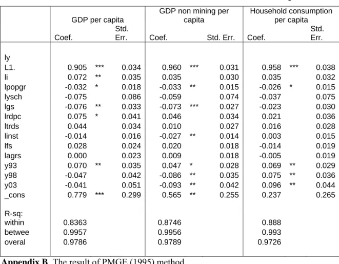
Nevertheless, there are two concerns in recent empirical development. First, Blundell and Bond (1998) show that the Arellano and Bond (1991) GMM procedure would have some downward bias if the left-hand side variable is persistent and the time dimension is small relative to number of individuals. The problem arises since the persistency in the data will make the lag value of this variable in level a poor instrument. In addition, with the small time dimension, there is not enough information available from the instrument.

Arellano and Bover (1995) offer a solution by adding the level equation back to the first difference equation. This will add information to the estimator that is crucial in determining the equation, especially if there is some time-invariant information that could be added. However, there is also an additional assumption needed to make this equation consistently estimated, which is

E [(ηi +uit ) Δxit] = 0 (16).

This means that there can not be any correlation between the individual effect and the change in the right hand side variables.

The other issue is in regard to the time length of the estimation. Pesaran, Smith and Shin(1999) show that, if the time length is relatively long compared to the number of individuals or regions, and there is an expectation of heterogeneity in the growth coefficient, the estimation using the Arellano and Bond (1991) dynamic panel

4 _{The endogeneity here is given by assuming the variable is weakly exogenous (Arellano and Bond}

1991)

5 _{Since equation (11) is the first difference there probably will be a first order serial correlation in the}

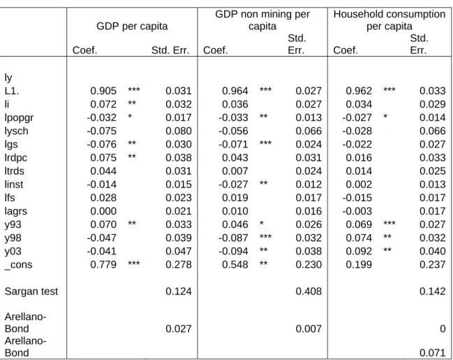
data estimate would have a misleading result. To deal with this problem the pooled mean group estimator (PMGE) should be implemented. This methodology works similarly to panel error correction model (PECM), however it relaxes the assumption of uniform coefficient across regions in the short term difference equation (Pesaran, Smith and Shin 1999).

3.2 The Sub National Application Issue

The regional or sub national analysis in growth studies has followed cross countries studies with three additional concerns: data availability, the impact of national policy, and interaction among regions. However, the concern will not be discussed in this chapter which will overview the first two in the case of Indonesia. Nevertheless, beside additional concerns, there are advantages in applying the empirical framework in sub national data especially for Indonesia.

3.2.1 Data availability

Since there are fewer boundaries of growth determinants in the literature, they could be any number of available explanation variables (Sala-I-Martin 1997, Levine and Renelt 1992, Durlauf and Quah 1999). Yet, not all variables used in cross country studies are available for a cross region study. This is partly because some variables may not be collected at the sub national level but is mostly because some variables are invariant in the district or provincial case. That is because they reflect national or central government policies and are uniform nationwide.

In particular, this chapter will discuss the availability of these variables in the Indonesian context. The big bang decentralization in Indonesia has changed the government system to become one of the most decentralised in the world. Even so, there are still eight functions that are coordinated and controlled by the central government - foreign affairs, defence, security, justice, monetary policy, fiscal policy and religion. In this case, it means most of the variables related to these functions may are uniform across the country. This is true for exchange rates, rule of law, external debt, and trade policies such as tariffs. In 2004, regions were expected the authority over external debt but this move was blocked by the Ministry of Finance.

Beside variables that are relatively uniform in the sub national context, there are some variables that would probably differ amongst regions but are not collected consistently over a long time period time. The main reason for is because the variable

is not considered important in the sub national context or is important only in a certain time period. One example is corruption. Before decentralization this variable was not considered important in the provincial context, since it was dominated by national corruption, so it was presumed to be arguably less important. Another example is conflict. Despite many localized conflicts in Indonesia since its independence in 1945, a record of the numbers and types of conflict is only available since major conflicts emerged in the late 1990s.

.

3.2.2 The impact of national policy

Growth studies at the sub national level also need to ascertain the impact on the national economy. National policy could have a different impact on different regions in Indonesia. For example, trade deregulation during 1986-1991 had more impact on regions that were already relatively open and had a high services share or exporting sector share in GDP. Nevertheless, there should be some national policies that have a common impact, such as budget expansion, family planning, compulsory primary schooling amongst others. This can also be seen from the previous chapter which showed that regional disparities were more or less constant. This implies most national policies over that period had a common impact on regional economies.

In a growth regression, all national impacts will be captured by the year dummies since they vary over time but stay the same across regions in one particular time. Nevertheless, the dummy will also capture world economic conditions. For the Indonesian case, it is reasonable to assume the impact of national policy or national economic conditions is more dominant than the impact of the world economy. Beside the role of the national economy is very dominant given the centralised nature of Indonesia, and the impact of world conditions would have an impact on the regional economy through the national economy. While this is not always the case, such as the impact of the oil price on mining regions, it is rare and past retention of oil revenue by the central government has minimized any direct impact.

3.2.3 The advantage of sub national studies

In Indonesia, most of the regional records come from the one source - the Indonesian Central Board of Statistics (BPS). One advantage is that the definition is uniform and comparable between regions in one particular time. Income is a good example. It is possible to have many proxies of income in sub national studies, since

the definition and collection processes are similar. On the other hand this is difficult in the cross country context since it is not just the recording process that could be different but also the way the income is distributed. Taking this as a consideration, three proxies of income could be used for this analysis - GDP per capita, GDP non mining per capita and household consumption per capita.

In the estimation issue, there are also some advantages in applying the empirical framework in sub national data especially for Indonesia. First, using sub national data means more justification to impose coefficient homogeneity than it does in cross country studies. In other words, it acceptable to expect the impact from one specific growth determinant is more uniform in one particular country rather than cross country.

Second, in Indonesia’s case, income per capita data are not persistent meaning income per capita has fluctuated considerably regionally. It is not only a case of having some fluctuations in the five yearly data but also in the annual data. As a result, it is acceptable to employ Arellano and Bond (1991) to do the estimation.

4. DATA

The data consist of 26 Indonesian provinces during 1983-2003 except for income proxy data start from 1978. As the dependent variable, income per capita will be the main variable in this analysis. The main database of income per capita is established from two Indonesian Central Board of Statistics (BPS) publications, which are the regional income accounts by production (value added) and by expenditure. The population data are taken from the CEIC Asia Database.

The data set start from 1983, because the expenditure approach data of provincial GDP start at that year. However the data for GDP and non mining GDP is started from 1978 as the estimation can use that lag data for instrumental variable. Another reason for using this time period is that the data before 1975 inconsistent and has major problem in some sectors. Arndt (1973) argued this was because the first effort of producing regional income data was from university economists rather than one central statistical official body. Although they worked closely with each other and according to BPS national income estimation procedure, there were some deficiencies

in the data source that would cause some inconsistency. The problem is more obvious in the sectoral estimation.6

4.1 Provinces

Some previous studies have addressed the concerns as to what level should be used to conduct regional analysis in Indonesia, since there are provincial and district/municipal levels. The chapter deals only with the provincial level despite the fact that in terms of regulation, decentralization has placed more power at the district level. The reason is that we would like to see the pattern since the 1980s and in the beginning the tension of imbalance development was built up at the provincial level. In the first 20 years of Indonesian independence, a weak central government in Jakarta had to face armed insurrection, i.e., separation movements, from several provinces, such as Aceh, West Sumatra, West Java, South Sulawesi and Maluku (Legge, 1961; Mackie, 1980). Note that recently separated East Timor was a province from 1976 to 1999. Also the on-going separation movements in Aceh and Papua are at the provincial level. It is therefore suspected that both the military and the central government were afraid more provinces would demand independence if greater power was given to them in decentralization.

Prior to July 1976, Indonesia consisted of 26 provinces and East Timor became the 27th province from July 1976 until August 1999. After the new laws on regional governance were passed in 1999, seven new provinces were proposed, but, until now, only four have been fully established, namely Banten in West Java, North Maluku in Maluku, Bangka Belitung in South Sumatera and Gorontalo in North Sulawesi. However, in order to have a continuous panel dataset from 1978 to 2003, these provinces have been regrouped to their original boundaries so there will only be 26 provinces in the dataset (i.e. excluding East Timor). However, it is important to note the regrouping of new provinces to the original has resulted in their GDP increasing dramatically in 2000. The possible explanation for this is that the separation of provinces means new investment for local government infrastructure and new employment for local civil servants, especially as they are all small units.

6 _{As an illustration, the manufacture sector in Jakarta was estimated to be very low at around 7 to 8%}

in 1969-1972before it became 12% in 1973, on the other hand, the trade estimate was too high during 1969-1974.

4.2 Income Proxies

As mentioned, income per capita plays the most significant role in this regression as it becomes the dependent variable. There are three income proxies that will be evaluated, provincial gross domestic product (GDP) per capita, non mining GDP per capita and household expenditure per capita. GDP per capita is the ratio of provincial GDP to total population. The data for non mining GDP per capita is calculated from the GDP per capita less mining sector value added per capita. The household consumption data are a part of the GDP by expenditure series.

The reason for three proxies is that use of GDP per capita has been criticized, on the grounds that most of the large mining output accrues to the central government and oil companies. Excluding the mining value added from GDP is one popular alternative income proxy. However, this proxy ignores any income or benefit from the mining sector that may go to local people. Especially in the analysis of growth determinants, the use of GDP per capita should be considered more appropriate than GDP non mining per capita. The main argument is that it is almost impossible to separate the mining component from most of the possible determinants that can be examined. For example, it is hard to exclude mining investment from investment data. This is also the case for the mining sector in human capital and trade.

Total household consumption is the third alternative. Household consumption shows how much welfare can be enjoyed by the whole household in a province. As a result, it can show the real income for the society regardless of the output taken by central or local government. The weakness of this proxy is that it does not reflect the value of a future income stream as a result of saving or investment. Moreover, the data are available only after 1983 instead of from 1975.

The data are in constant prices, as in cross country and intra country studies. This is applied since the real growth of these regions will be measured which is supposed to be the growth of goods and services. All three proxies will use constant 1993 prices.

5. DETERMINANT OF GROWTH

Durlauf and Quah (1999) stated the growth determinants are the explanatory variables of total factor productivity. These could be any differences among region but there are some variables commonly used in cross country studies that cannot be used in sub national studies especially for Indonesia. Two obvious causes are because

the variables are not available in sub national data or are invariant amongst them. The number of variables will be further reduced due to data availability. The main

variables are as follows:

5.1 Investment

Investment is one variable directly implied by the Solow-Swan growth model. In terms of total output share, it represents the saving of physical capital in the economy, as can be seen in equation (8). In the model, physical capital investment could enhance both the income level in steady state or a balanced growth path and also the speed in achieving it (the growth level). Therefore, the Solow-Swan model should also be applicable for any level of the economy including sub national. Investment is important potentially growth determinant in this study.

This theory is supported by the empirical results that estimate the robust positive impact of investment on growth (Barro 1991, Caselli et.al. 1996, Levine and Renelt 1992, Mankiw et.al. 1992, Sachs and Warner 1995). Nevertheless, the inclusion of human capital shows the superiority of this variable may not be as strong as earlier predicted (Mankiw et.al. 1992). Moreover, the direction of causality could be from growth to investment rather than vice versa (Blomstrom, Lipsey and Zejan 1993). Barro (1996) shares this view in pointing to high growth prospects as the reason behind high investment. their result came with a different sign, i.e., positive in Barro (1996) but negative in Blomstrom et. al. (1993). However Both these studies have concluded the insignificant impact of investment.

Investment in term of gross fixed capital formation as proportion of GDP is also examined in sub national studies. However, the result is not as convincing as the cross country studies, even when it is treated as exogenous. For example, Ferreira (2000) finds it was insignificant for Brazil during 1975-1990. The same result is also found by Klump and Nguyen (2004) for Vietnam during 1995-2000. This could only be developing country phenomena, since it was found to be positively significant for Australia in 1991-2000 (Ramakrishnan and Cerisola 2004). Yet, their separate estimate for 1991-1996 showed investment to be insignificant.

The data for investment in term of gross fixed capital formation are also available at the provincial level in Indonesia. They can be taken from the regional (provincial) income account by expenditure in BPS dataset. Given the model

indicated the uses of investment rate then the ratio of gross fixed capital formation to Gross domestic Product is used for the variable.

Nevertheless, more recent studies have argued that the accumulation of physical capital alone cannot explain the growth of income differences to the degree indicated by the Solow-Swan growth model. Hence, there are further steps to seek more explanation from the role of capital in growth. As investment itself consists of many kinds and types of capital, one of the required steps is to analyse the performance of these different kinds of investment or capital in the economy. This could be within the physical capital or by the addition of other capital such as human capital.

5.2 The Interconnected Investment Variables

Infrastructure and government spending are two factors predicted to have some impact on growth. Ironically, these two kinds of investment were initially introduced as one component of investment, public provision of core infrastructure (Aschauer 1989). He pointed out that public provision of core infrastructure, such as streets, highways, airports, mass transit systems, electricity, gas, water and sewerage, has a positive spillover effect on productivity, meaning the existence of this infrastructure could make other capital work more efficiently. An example is the argument built by Henderson (2000) that this infrastructure is important in lowering the transportation and instalment cost of capital.

However, there is a negative impact of public provision from government spending. Barro (1990) has pointed out the crowding out effect from taxation is the main reason for this negative impact. This was also discussed by Aschauer (1989) who said it will happen especially in the short term analysis. However, recent studies find the negative impact is also the result of public expenditure composition as summarized by Folster and Henrekson (1999). First of all, allocation of public expenditure is more on social welfare activities, subsidies and transfers that are not related to the growth process and even discourage it in terms of less saving and job seeking. Furthermore, sometimes this investment competes with private investment in term of resources like land or buildings. The worst case is if public investment is allocated to an activity that could excite private activity like maintaining the bureaucracy. Regional Indonesian economies should also have experienced this type of investment given the high level of bureaucracy in the past.

The distinction of these variables was also not clear in beginning of empirical studies. Aschauer (1989) used government spending from the national income and product account of the USA during 1949-1985. Munnell (1990) followed this with an estimation of pooled data from 48 US states during 1970-1988 and also came up with a positive significant impact from government spending. However, this was only local spending and did not take account of the federal spending in these states.

On the other hand, Barro (1991) found a negative impact from government spending in cross country studies. Yet, he used government consumption excluding education and defence as the government spending. Barro (1991) also introduced government investment and found it to be positive but insignificant. Levine and Renelt (1992) used the various expenditures of government to show a negative impact which was not robust in their criteria. Sala-I-Martin (1997) also showed that even government investment was insignificant and the sign could be positive or negative depending on the other variables used. Folster and Henrekson (1999) also pointed out the potential problem from having a variable funded by government spending at the same time as investment in the growth regression.

In sub national studies, Higgins et.al. (2003) has analyse the size of government in the economy using the proportion of people employed by local, state and federal US government. The used of three level of government is based on the argument that the higher level of government would react slowly to people need and become less productive. Meanwhile, they used the proportion of employment since they found that public infrastructures and services are likely to have externalities to other regions. Esquivel and Messmacher (2002) have included telephone density as growth determinant for Mexico but it turns out to be insignificant.

So the major issue is how to address the fact that the investment variable will contain government investment and infrastructure. The colinearity among those variables can be an important source of information as to how the variables impact with each other and can also provide an explanation for the performance of one of the variables when the other variable is not controlled.

The other issue is to pick the infrastructure that really is important for the Indonesian economy and has reasonable data availability. Given that Indonesia overall is still in the developing stage, a transportation measure is considered more important since other infrastructure can only work or be installed if there is transportation in place. So this chapter will focus on the infrastructure that is closely

related with transportation. We argue that road per capita is the most reliable data for this. It is the ratio of length of road to population including asphalt and non asphalt. There is actually another roads dataset in Indonesia, based on the level of government expenditure maintaining the roads. Nevertheless, the total length of the road is used. Data on length of roads have been available since 1973/1974 five years development report, and the annual data are available since 1980 for all provinces except Jakarta where it is only available after 1992. Therefore, length of roads for Jakarta is estimated assuming that the growth of length of roads is constant.

Government spending will be represented by its development budget. Although the data for the overall development budget have never been broken down to provincial level, there are data in both the provincial and district budget, so both can be used to represent the government budget. Even though the data contain INPRES expenditure from the central government, this will not capture a significant proportion since a major component is directly invested by central government agency to the region. The data for provincial budgets have been available since 1969 while accumulated data for district budgets have been available since 1982.

5.3 Human Capital

Human Capital has become a common suspected growth determinant especially as measured by education. Lucas (1988) defined human capital as the general skill level, indicating that human capital contributes to growth by increasing worker productivity besides also increasing output through its externality. The impact of human capital accumulation also contributes to higher technical progress by affecting knowledge accumulation (Romer 1990), lowering population growth (Becker, Murphy and Tamura 1990), or both (Galor and Weil 2000). As a result, human capital should have a positive impact on growth and could even be the major engine of per capita income growth (Mankiw et.al. 1992).

Given the hypothetically important role of human capital accumulation, it has been considered one of the major causes of unequal development achievement across countries, and even across regions within a country. Conversely, it can be seen as a way to solve the inequality problem by increasing or giving subsidy for the education of poor people or regions. Mankiw et.al. (1992) is the first well known empirical study that strongly supports this claim. They even show the role of human capital is actually higher than the role of physical capital.

However, as the empirical techniques have developed the result has varied. For example, Islam (1995), using panel data technique, discovered an insignificant relationship between level of human capital and income per capita growth. This was followed by Pritchett (1999), although he argues the relationship actually exists but is covered by generalization of the data set since the impact of education was not the same for different classifications of countries. In particular, education could have a negative impact on growth due to poor quality of schooling, or lack of demand for schooling.

The sub national studies have found more positive results. Ferreira (2000) use an average year of schooling variable to conclude that education has a positively significant impact on sub national growth in Brazil but may not be linear. Higgins et.al (2003) analyse education with the percentage of people that completed college and a bachelor degree or higher as two separate variables. While a bachelor degree is strongly positive for US growth, college education came up with a mixed result. It seems to be positive for non metro areas but negative for metro areas although neither is significant.

The positive impact of human capital on inter-provincial growth differential continues to be a widely held belief within official circles in Indonesia. It can be seen by the effort to increase literacy and to at least propose a compulsory education level of primary school in the Suharto era and junior high school in the present day. The expectation of a positive impact is strengthened by Garcia and Sulitianingsih (1998) using the average years of schooling as the proxy for education. Nevertheless, they also note the impact becomes weaker after 1983. One the possible reason is that the level of education has become more uniform in the recent year.

As the role of human capital focuses on education, average years of schooling will be the proxy for the variable. The data are taken from the education of people over 10 years of age in the Labour Force Situation in Indonesia series which is the result of a National Labour Survey (Sakernas) from BPS. There are eight categories in this case starting from no schooling, not yet completed primary school, completed primary school, completed both general and vocational junior high school as well as senior high school, academy/diploma, and finally university. The percentage of each category is then weighted by the years needed to complete that education level. The first and second category will have 0 as the weight, the third will have 6, the

completed junior high school criteria will have 9, senior high school will be 12 and a diploma or university will be 15.

The other issue in this data base is the completeness of the data for entire periods. Sakernas was not conducted in 1981, 1983, 1984, and 1993 while 1980, 1985, 1990 and 1995 have to use data from a limited population survey conducted between censuses. There is also the issue of the change of labour force ages criteria since 1998 from 10 to 15 years old, but that has not become a problem since the raw data is available. The data for the missing years have to be estimated and this is done by interpolation.

5.4 Openness

Openness is another important engine of growth since the integration of economies will provide a greater trade in goods and flow of ideas (Rivera-Batiz and Romer 1991). Sachs and Warner (1995) have more specifically claimed that openness will facilitate the gains from international trade. They argue that countries with liberal trade policy will have relatively better economic growth. Specifically, they define openness as the absence of non tariff barrier, more than 40% tariff rate, and a significant black exchange rate market, socialist economic system, and state monopoly of major export. Sachs and Warner (1997) used landlocked as a variable that contrasts with openness.

An alternative measure of openness is the ratio of trade to GDP. This measurement has a weakness due to the endogenity problem as the higher growth would mean greater pressure to trade. Nevertheless, Frankel and Romer (1996) counter this argument by saying endogenity can be solved using an instrument variable. On the other hand, a trade policy variable has its own problem as it is likely to be correlated with the omitted variable. The trade policy is likely to have a strong relationship especially to the domestic market and fiscal condition that cannot be correctly addressed. As a result, it may produce a bias estimation.

The empirical results show the impact of openness in term of trade size is significant. Sala-I-Martin (1997) found a significant positive growth impact from the time an economy has been open, but Barro and Lee (1994) found the negative impact from tariffs barrier to not be significant. On the other hand, Frankel and Romer (1996) recorded a significant positive impact on growth from trade size.

Not many sub national studies have used an openness indicator as a determinant of growth. Basically, the trade policy indicator is irrelevant since it should be uniform within a country. Another possible reason is the international export-import database of a region is difficult to obtain since the subject of international trade is a country rather than a region in a country. Nevertheless, Raiser (1998) examined the impact of a coastal area dummy for China and found a significant positive impact on growth.

In Indonesia’s case, international trade data in a region can be obtained from industrial statistics, but they will only contain the manufacturing sector. Amity and Cameron (2003) confirmed the significance of this trade and argue that market and supplier access determines industrial income in districts of Indonesia. Temple (2002) has even identified fast growth of trading partners as a reason why Indonesia could have experienced high growth in the past. From these arguments, it is clear that openness would benefit Indonesia especially in term of trade and possibly in market access.

Regarding to the difficulty in obtaining the international trade data for region, the overall trade that included the domestic trade could be used. One basic argument is that the domestic market may also be important in boosting regional growth. There would be a disadvantages since the level of competition in doing international trade will be much greater than domestic competition and also the possibility of technological transfer from international knowledge. Nevertheless, the domestic trade can provide the competition and information access to some extent and hence have an impact on growth in a region.

Provincial trade data are available form BPS. It can be taken from regional income account by expenditure. Data contain exports and imports as well as consumption and investment and is available from 1983. Export and import in the database will contain the trade activities of a region to other including international as well as domestic. The trade indicator will be the ratio of the sum of exports and imports to GDP.

5.5 Institutions

The role of institutions has become the influential factor in boosting economic growth. The scope of institutions has become very wide (Sala-I-Martin 2002) and can be measured with various proxies (Glaeser et.al 2004). The usual definition of an

institution is a set of rules, procedures and norms that determines commercial behaviour (North 1981). It means a good institution is expected to give an incentive for the economy to be more productive (Kong 2006). Sala-I-Martin (2002) includes law enforcement, market function, inequality, conflicts, political institutions, the health system, financial institutions and government institutions in this new engine of growth. Accordingly, institutions not only considers rules or values that could give more incentive but also ones that could cause disincentive.

One direct proxy to measure institutions is the measurement of norms or rules implemented in a particular economic society. The rules held by that society determine the levels of efficiency and effectiveness and hence decide overall economic performance. The existence of property law and the degree of the role of law are often used as an indicator. The social norm could, as a more abstract measure, be measured by the percentage of certain ethnic groups or religions, since most of the rules come from cultural and religious beliefs. This also actually measures the level of homogeneity in the society as an institution measure.

Although coming with various measures, the existence of laws or norms as institutions usually has a positive impact on growth. Rodrik et.al. (2002) has strongly supported the positive impact hypothesis by showing the significant result from a composite index that contains property law and rule of law. Nevertheless, Sala-I-Martin (1996), explicitly explored most of the variables in cross country study and found that the rule of law, percentage of Confucian and percentage of Muslims are positively significant while, political rights, civil liberty and revolution are negatively significant. Acemoglu et.al. (2001) had an interesting result as they highlight that colonial origins has affected the form of present institutions and hence show strong determination to income per capita.

Institutions are not commonly included as a sub national growth determinant. One of the possible reasons for this could be that the sub national institution for many countries is considered invariant. For example, most countries have the same origin of colonialism, rule of law and political right. However, for a country like Indonesia that has a great variance of culture it is important to recognize the difference in culture and it is change over time. One study for sub national growth that has the institutional variable is for the Philippines (Balisacan and Fuwa 2003). They use the political institution called ‘dynasty’ defined as the proportion of government officials related

to each other by blood or marriage. The variable has a significantly negative impact on growth.

The same cannot be done for Indonesia because the data not available. Cultural background best option for Indonesia, but the questionnaire of the census has asked different things regarding cultural background from time to time. So second best is to use the fraction of religion. In this case the proportion of Muslims is used as the largest community in Indonesia. The data are available from the 1990 and 2000 population census. The data for 1980 and 1985 are available in the statistical yearbook of Indonesia.

5.6 Financial Institution

Another institution that has an impact on growth is financial institution. Nevertheless, institution in this case means organisational bodies rather than a set of rules and norms. The role of financial institution was first raised by Schumpeter (1912). He revealed the significant role of financial intermediaries in economic development since they make the allocation decisions of a community’s saving. Yet, other economists have since argued that financial intermediaries also influence the rate of savings and eventually influence capital accumulation and growth (King and Levine 1994) or the combination of both (Levine 1999). So the impact can be through capital accumulation as well as through productivity. However, the growth examination that includes capital accumulation as one of the growth determinants will only provide an answer on the impact from the productivity side.

The empirical study on the impact from financial intermediaries’ size on growth has begun very early. Goldsmith (1969) revealed the positive impact of this variable but as the growth regression is yet to be introduced; it failed to explain how it happens. From the empirical studies on financial institutions after that, King and Levine (1993) was first to examine financial institutions in terms of size. There were four measurements used in this study. These were the currency plus intermediary’s liabilities per GDP (DEPTH), the ratio of bank credit to the sum of bank credit and central bank asset (BANK), the ratio of private enterprises credit to total domestic credit (PRIVATE), and the private enterprises credit divided by GDP (PRIVY). The results of 74 countries that have complete pooled data showed there was a strong positive relationship between these four measurements and growth, capital accumulation and productivity although the direction of causality not clear.

Sub national empirical study on financial institution impact on growth is rare. Higgins et.al. (2003), used employment in finance to overall employment to see this impact and found a weakly significant positive impact. Nevertheless, there are some studies that examine the issues by groups of countries in one geographical area. De Gregorio and Guidotti (1995) presented evidence that the positive relationship in a cross-sectional worldwide sample of countries was turning into a negative relationship in panel regressions for only Latin American countries. They argued that it was due to the impact of repeated financial crises and overlending problems that the region had suffered. Athukorala and Warr (2001) also showed that the private credit to GDP ratio (PRIVY) increased sharply in Indonesia, Korea, Malaysia, the Philippines, and Thailand before the crisis struck.

The topic is actually very crucial for Indonesia since financial institution has developed very unevenly. From the share of GDP, the financial sector has been around 20-30% in Jakarta and 12% in Jogjakarta and below 3% in 7 other provinces. Indonesia is fortunate to have the data on provincial savings and credit in the commercial bank data. It has been collected and published by Central Bank of Indonesia since 1985 in Indonesian Economic and Finance Statistics. The disparity in the amount of savings and credit per GDP is more severe in this case. It is above 100% for Jakarta and below 10% in 5 other provinces. Jakarta has managed to have the very large size of financial institution because of almost all headquarter of big company in Indonesia is in Jakarta. This is also the result of centralised approach of government in the past.

5.7 Economic Structure

Economic Structure or share of some sector role in the sub national growth economy is often considered important. It has been done since the empirical studies pioneered by Barro and Sala-I-Martin (1991). The variable is capable of capturing the existence of a specific sector that behaves differently but more importantly can control the large shift in economic structure that could suddenly change the convergence pattern as well as the performance of growth determinant (Barro and Sala-I-Martin 1991). They examined the data after World War II and confirm that the shift of the agriculture sector was the main source of this effect.

For the above reason, it is important to include the variable in the growth regression. The main argument is Indonesia during 1983-2003 shifted extensively

from a pre dominantly agricultural economy to more manufacturing industry, as well as the fact that agricultural productivity in Indonesia may not be as responsive as other sectors to the growth determinants.

Finally, the data for agriculture share are taken from the provincial income account by sectors. So they are the share of value added of the agriculture sector in the GDP as total value added. As mentioned earlier, these data are actually available from 1969 but are more reliable after 1975. All of these data will be treated as logarithm value in the estimation process as it will follow closely with the theoretical model in equation (8).

6. EMPIRICAL ESTIMATION

As the potential growth determinant is identified, the empirical equation can be formed. The growth determinant will be part of matrix ZTit in equation (10). As a

result the growth equation can be estimated as follows:

lnyit = γ1 + γylnyit-5 + γ3ln(s)it + γ4ln(n)it+ γ5ln(ysch)it + γ6ln(gs)it + γ3ln(rdpc)it +

γ4ln(trds)it + γ3ln(inst)it + γ4ln(fs)it + γ3ln(agrs)it + ∑dyt + ηi + uit (10)

Where :

yit is proxy of income of province i at time t, which are GDP per

capita, non mining GDP per capita, Household consumption per capita (million of Rupiah, 1993 prices)

sit is the Investment (gross fixed capital formation) share over

GDP of province i at time t

yschit is the average year of schooling of the total population above

10 years of ages at time t to represent the stock of human capital (years)

gsit is the local (Province and district) development expenditure as

a share of GDP to represent government spending in province i at time t

rdpcit is the length of road per population to represent infrastructure

trdsit is the ratio of total trade (Export plus Import) to total GDP to

represent openness in province i at time t.

instit is the ratio of Muslim to total population to represent the

institution and its homogeneity in province i at time t.

fsit is the ratio of total savings and credit in commercial banks to

total GDP to represent the size of financial institution in province i at time t.

agrsit is the ratio of agriculture value added to total GDP to control

the impact of structural change in province i at time t. dyt is the dummy for time periods

1 88 = d if t=1988, or 0 otherwise 1 93 = d if t=1993, or 0 otherwise 1 98 = d if t=1998, or 0 otherwise 1 03 = d if t=2003, or 0 otherwise The base period is year 1983.

ηi is the provincial fixed effect (unobserved heterogeneity)

6.1 The Performance of Estimation

The Sargan test of over identifying restriction and the residual autocorrelation test are the main quality insurances of the Arellano and Bond (1991) dynamic panel GMM estimation method. The Sargan test will basically tests whether the restriction on the moment condition needs to be rejected and cannot be used. So if the degree of rejection is not strong enough the estimation result can still be used. The significance level that will be used to examine this is 10%. In the case of autocorrelation, the first order error correlation is actually expected since the estimation is conducted on the first difference equation. As a result, there will be autocorrelation of the first difference of error in time t with the first difference in time t-5, since both have error at time t-5 as its component. Nevertheless, there should be no autocorrelation in the second order correlation.

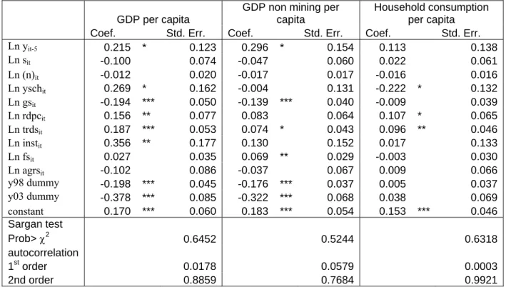
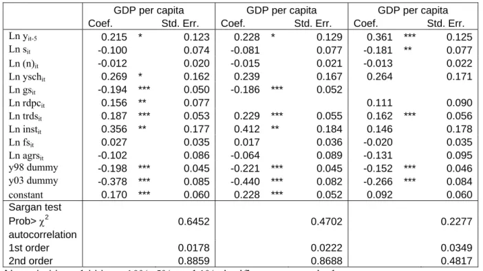
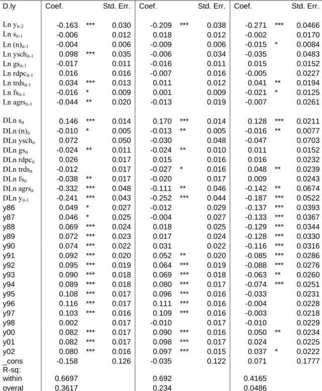
The Sargan test on the estimation with the assumption of exogenous independent variable has resulted in rejection of the GDP per capita and GDP non mining per capita estimation but not of household expenditure per capita. The significant level of the rejection on the GDP per capita estimation is 4.9%, indicating

the existence of endogeneity in the independent variable. The result is reasonable since the growth of income will at least determine investment, education attainment, infrastructure (road) and financial institution. Nevertheless, there are no problems regarding the autocorrelation of this estimation. The test indicates the existence of a first order residual autocorrelation but not a second order autocorrelation.

On the other hand, the Sargan test for GDP non mining and household consumption are actually acceptable with a 48.0% and 70.1% of significance level. Nevertheless, the result also shows there are no first order autocorrelations neither of these two proxies. This is unusual since the construction of the Arrelano and Bond (1991) estimation expects correlation in the first order condition.

The exogeneity assumption is loosened for all dependent variables in the next estimations. It is done by setting all dependent variable to be pre determined meaning they are instrumented by their lag. These estimations give more accepted results. The Sargan test for the estimation of GDP per capita, GDP non mining per capita and household per capita all fail to reject the restriction in moment condition with a significance level of 64.5%, 52.4% and 63.18%, respectively. Furthermore the first order residual autocorrelation is existed for all estimations in but not the second order.

6.2 The Determinant

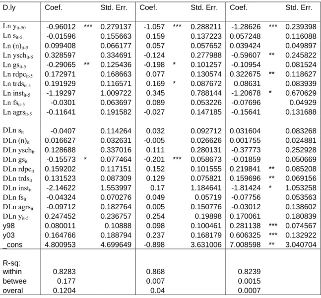
The accepted results show that the significant growth determinants are different for different income proxies. Nevertheless, the significant growth determinants of GDP non mining per capita are also significant for GDP per capita, except for the financial institution. Meanwhile, the growth of household consumption per capita seems to have different determinants that are related to the spending behaviour of households rather than as a proxy of income. The significance of these variables will be discussed first before analysing their interpretation.

Investment is estimated to have an insignificant impact on growth of all the income proxies. Its coefficients have negative sign in the estimations for GDP and GDP non mining, but are positive for household consumption. The result could be explained by the endogeneity argument, since it has been treated as endogenous in the estimation. Nevertheless, the results in the estimation that set the variable to be exogenous also have an insignificant impact.

So these results are better compared with the results from Vietnam and Brazil. The results from these two developing countries show the insignificance of the

investment impact on growth. The argument could be taken from the fact that investment still contains a significance percentage of government investment that could have an insignificant impact or even a negative impact on economic growth. This issue will be discussed further in the independent variable inter-correlation.

The average years of schooling has a different impact on different proxies of income. It is weakly positively significant on GDP growth, insignificant on GDP non mining and surprisingly negatively significant on household consumption. The weakly significant impact on GDP growth is similar to the result from Garcia and Sulistianingsih (1995). Although positively very significant in the 1975-1993 estimation, school attainment becomes insignificant in the 1983-1993 estimation. The argument of a massive increase in primary school graduation could explain this decreasing impact of education given the possibility of diminishing marginal impact.

On the other hand, the insignificant impact on GDP non mining can be explained by the fact that the data contain the school attainment of all employment including the mining sector. Even though the share of mining employment is not big the average year of schooling should be very high because as the mining sector is operated by a big and high capital company, they will employ many labours with tertiary education. So even if the growth of non mining sector is low in the mining rich province, it still take the contribution of the highly educated mining labour into account.

Meanwhile, the story is completely different for household consumption per capita. Surprisingly, there is a weakly significant negative impact on growth from the average years of schooling. However, it will be less surprising if consumption is seen as spending behaviour. People with education are usually more cautious in consuming their money as they have begun thinking about saving and investment.

There are negative impacts on growth from local government spending on GDP per capita and GDP non mining per capita. Given the tax is taken by the central government while the spending is local, the argument of crowding effect may not be relevant. Government spending could actually have a negative impact either not boosting growth in five year period in a five years period or even restricting growth as discussed earlier. From the development budget of provincial and district government, only 50% to 60% is allocated to infrastructure. The other 50-40% allocated mostly to

government apparatus or bureaucracy (14%) and social activity for youths and teenagers (7%).7

On the other hand the impact of transportation infrastructure in terms of road per capita is significantly positive on GDP per capita growth. Although weak, the impact is also significantly positive on household expenditure. These results are expected, since the existence of roads will lower transportation cost and increase mobility in the region and so showed increase growth in both output and consumption. Yet, it is surprising that the impact on non mining GDP per capita is insignificant. The most plausible reason for this is that a significant amount of roads per capita are built and used for mining purposes. This reason is acceptable in remote areas where mining activity takes place, but roads in a place like Java are certainly used by the non mining sector. Yet the number of population in that area is relatively large so that roads per capita are relatively small.

The ratio of trade to GDP, as a proxy of openness, is another significant growth determinant. The trade share is estimated to have a very significant impact on growth of GDP per capita as its significant level is less than 1%. Actually, the variable has shown more of the gain of trade of each province since it also contains trade with other regions and not necessarily just with a foreign country. The impact is weakly significant for GDP non mining. One possible reason is that the variables still contain mining sector trade. For example, the export-import statistics from BPS indicates that more than 30% of Indonesia’s export and import comprises mining related commodities. Trade is also a significant determinant for household consumption growth. Besides being acceptable in explaining the growth of income, trade share is also very reasonable in explaining spending behaviour. Trade will open the opportunity for new goods and services from outside regions to come in so that people have more spending choice.

The result from the institutional variable is very interesting. It is positively significant for GDP per capita but not significant for GDP non mining and household consumption. While it is reasonable for household consumption, since there is no significant difference in the spending behaviour of Muslims and non Muslims in Indonesia, the difference between the results in GDP and GDP non mining is hard to explain. First, not all mining provinces are Muslim dominated. Over 95% of Aceh’s

7 _{The rest is allocated to social sectors such as family planning, information and communication and}

population is Muslim, Riau had 92% in 1980 but decreasing to 88% in the 1990s while East Kalimantan and Papua only had around 85% and 20%, respectively. Although the variable shows an indicator of homogeneity, even conflict cannot explain the relationship with growth.

In contrast, the financial institution is only significant for GDP non mining. The result can be explained as follows, the majority of mining corporations do not start their business by borrowing from local financial institutions so the impact of financial institutions is not large if mining is taken into account. This can be seen from the size of local financial institutions in Aceh, Riau, East Kalimantan and Papua in 1985 which was 6.4%, 4.3%, 5.5% and 9.6% of GDP respectively compared to Jakarta (150%), or even East Java (23%). Yet the growth of financial institutions is also high as all of those mining rich provinces have more than a 20% financial institution size of GDP in 2003. Nevertheless, the highest growth was in Riau, rising from 4.3% in 1985 to 46% in 2003. The impact is not significant for household consumption, since although the credit could boost the expenditure, saving works in the opposite direction.

Table 1. Results for the Arrelano and Bond (1991) Dynamic Panel Estimation on Growth Regression

GDP per capita

GDP non mining per capita

Household consumption per capita

Coef. Std. Err. Coef. Std. Err. Coef. Std. Err.

Ln yit-5 0.215 * 0.123 0.296 * 0.154 0.113 0.138 Ln sit -0.100 0.074 -0.047 0.060 0.022 0.061 Ln (n)it -0.012 0.020 -0.017 0.017 -0.016 0.016 Ln yschit 0.269 * 0.162 -0.004 0.131 -0.222 * 0.132 Ln gsit -0.194 *** 0.050 -0.139 *** 0.040 -0.009 0.039 Ln rdpcit 0.156 ** 0.077 0.083 0.064 0.107 * 0.065 Ln trdsit 0.187 *** 0.053 0.074 * 0.043 0.096 ** 0.046 Ln instit 0.356 ** 0.177 0.130 0.152 0.017 0.133 Ln fsit 0.027 0.035 0.069 ** 0.029 -0.003 0.030 Ln agrsit -0.102 0.086 -0.037 0.067 0.009 0.066 y98 dummy -0.198 *** 0.045 -0.176 *** 0.037 0.005 0.037 y03 dummy -0.378 *** 0.085 -0.322 *** 0.068 0.038 0.069 constant 0.170 *** 0.060 0.183 *** 0.054 0.153 *** 0.046 Sargan test Prob> χ2 0.6452 0.5244 0.6318 autocorrelation 1st order 0.0178 0.0579 0.0003 2nd order 0.8859 0.7684 0.9921

As discussed, a common impact of national macro economics conditions on provincial growth can be seen from the year dummy variables. These year dummy variables are very significant for GDP and GDP non mining but not for household consumption. This means the performance of the national economy and hence the general world economy would determine the condition of a particular province. This is not surprising for a country that used to be centralised in its governance. The interesting thing is that this national macroeconomic situation has not significantly affected the pattern of household consumption.

6.3 Interpreting the Coefficient

It is important to notice that there are two ways to interpret this coefficient which actually have the same end result. The duality of interpretation can be a result of two empirical equations constructed from equation (8), which is the basic model. This has been incorporated with equation (9) and (10) to be applied in the estimation. Although in the first instance the interpretation seems different it should actually have the same end result since both came from equation (8).

Taken from equation (9), the estimation has been applied to the equation of ln(yit /yit-5) = γ1+γ2lnyit-5+∑γx ln(x it)+ +∑γz ln(z it)+ ηi+uit (15)

so the interpretation of coefficient is

) (z ) (z ) /y (y ) /y (y ) ln(z ) /y ln(y it it 5 -it it 5 -it it it 5 -it it Δ Δ = ∂ ∂ = z γ ,

which means that γz shows the impact of the percentage change of z it on the

percentage changeof (yit /yit-5) and not the percentage change of growth.

It is still possible to know the impact on growth, if the current rate of growth is known, since the impact on growth will be equal to (yit /(yit - yit-5)) times γz. So if a

region grows 25% in 5 years (approximately 4.6% annually) the impact on growth is 4 times γz. In this case for GDP per capita, a 1% increase in the average years of

schooling in five years will increase growth by as much as 1.08% from 25% to 25.27% in five years or from 4.56% to 4.61% annually given that all other variables are controlled. However, although years of schooling is estimated to have such a high impact the impact is very uncertain as it is weakly significant since the standard error is also high.

On the other hand, the interpretation can also be done using equation (10) which basically is

ln(yit ) = γ1+γylnyit-5+∑γx ln(x it)+ +∑γz ln(z it)+ ηi+uit (16)

meaning the coefficient can be interpreted as

) (z ) (z ) (y ) (y ) ln(z ) ln(y it it it it it it Δ Δ = ∂ ∂ = z γ

so in this case, γz shows the impact of percentage change of z it on percentage change

of (yit) or in other words, growth of z it on growthof (yit).

However, it will actually give the same result. Taking the same example, growth in the average years of schooling by as much as 1% in five years will increase the growth of income by 0.27 percentage points. This direct interpretation seems different from the first. Yet, setting current growth to be 25% in 5 years will change the growth to 25.27% or from 4.56% to 4.61% annually. So the interpretation is actually the same.

In the interpretation, it is necessary to mention the significance of the variable, since the variable with high magnitude is not always the most significant. The significance level is taken from the position of the ratio of the magnitude of the coefficient with its standard error. As a result, it has taken account of the certainty of the impact. For example, the impact of a 1% increase in trade share on growth (0.19 percentage point increase) is smaller compared to the impact of a 1% increase in average years of schooling (0.27 percentage points of growth) but the standard error is far lower, so the possibility of the impact realised is bigger. This could make the trade share is preferable for the policy maker.

Meanwhile, the highest magnitude of positive impact on GDP growth is actually given by the institution proxy (Ln instit). The standard error of the coefficient

is also not too far from the average years of schooling, so there is still an acceptable level of certainty. However, although the magnitude of the institution impact is also high on the GDP non mining growth, the level of uncertainty is far above the other determinants and the magnitude of its impact is very low on household consumption.

The two significant growth determinants for GDP non mining actually have low magnitude. The coefficient of financial institution and trade are lower than the coefficient of institution and roads per capita. Using the same assumption of 25%