Policy Research Working Paper
5256
Time Allocation in Rural Households
The Indirect Effects of Conditional Cash Transfer Programs
Amer Hasan
The World Bank
Latin America and the Caribbean Region
Poverty and Gender Group
March 2010
Impact Evaluation Series No. 43
WPS5256
Public Disclosure Authorized
Public Disclosure Authorized
Public Disclosure Authorized
Abstract
The Impact Evaluation Series has been established in recognition of the importance of impact evaluation studies for World Bank operations and for development in general. The series serves as a vehicle for the dissemination of findings of those studies. Papers in this series are part of the Bank’s Policy Research Working Paper Series. The papers carry the names of the authors and should be cited accordingly. The findings, interpretations, and conclusions expressed in this paper are entirely those of the authors. They do not necessarily represent the views of the International Bank for Reconstruction and Development/World Bank and its affiliated organizations, or those of the Executive Directors of the World Bank or the governments they represent.
Policy Research Working Paper 5256
Conditional cash transfers are being heralded as effective tools against the intergenerational transmission of poverty. There is substantial evidence on the positive effects of these transfers. Analysts are only now beginning to investigate the indirect effects these programs generate. This paper examines the effect of a gender-targeted conditional cash transfer program on the time allocation of mothers in rural program-eligible households. Using a fixed effects difference-in-differences estimator, the
This paper—a product of the Poverty and Gender Group, Poverty Reduction and Economic Management Sector of the Latin America and Caribbean Region—is part of a larger effort in the department to evaluate the full range of impacts social programs produce. Policy Research Working Papers are also posted on the Web at http://econ.worldbank.org. The author may be contacted at [email protected].
author finds that program eligibility is associated with an increase of 120 minutes of housework per typical school day by mothers of eligible children in the stipend district when compared with mothers of eligible children in the non-stipend district. There is a 100-minute reduction in the amount of time mothers report spending on children’s needs. The intent-to-treat effect of the program suggests no change in the amount of time spent on paid work or sleep.
Time allocation in rural households:
The indirect effects of conditional cash transfer programs
Amer Hasan
Poverty and Gender Group
Poverty Reduction and Economic Management Unit Latin America and the Caribbean Region (LCSPP)
1850 I Street, NW Washington, DC 20433
I would like to thank Dan Black, Jishnu Das, Asim Khwaja, Robert LaLonde, Robert Michael and Marcos Rangel for helpful discussions on the topic. Haeil Jung, Daniel Kreisman, Patrick Wightman provided valuable feedback on earlier versions of this paper. All remaining errors are my own. Mohsin Chandna and Syed Sohail Raza were instrumental in gaining access to the administrative data used in parts of this paper.
I. Introduction
Over the course of the last decade conditional cash transfer programs (CCTs) have become a popular policy instrument in combating the inter-generational transmission of poverty. As the name suggests these programs entail transferring cash to beneficiaries provided they alter their behavior according to pre-defined conditions. Typically these conditions relate to human capital investments in children. Consequently, this policy instrument is seen as tackling poverty in the current generation via the transfer and in the subsequent generations via increased human capital investments in children.
The heightened excitement in policymaking circles stems in large part from a substantial body of active academic research which suggests that these programs are an effective means of increasing human capital investments in children. This research has been instrumental in updating existing programs and in refining new ones. However, much less is known about the unintended consequences these programs might have. It is particularly important for this gap to be filled as new programs are introducing new forms of targeting. The focus of the present paper is the use of gender-targeting to determine program eligibility.
It is well-documented that in rural households, school-age girls are extensively engaged in household chores.1 When conditional cash transfer programs are implemented in rural areas and girls take up the chance to go to school, it stands to reason that they have less time to spend on work around the house. This raises the following question: who does the work these girls would have been doing in the absence of the program? Does the household respond by allocating chores to a different sibling or does the mother adjust her time allocation? A complete
1
Levison et. al. (2001) and Ersado (2002) show that workloads are heavier for girls than for boys according to a range of definitions of work and in a multitude of regional and national settings. See also the evidence presented in Cynthia B. Lloyd et. al., 2008 and the references cited therein.
understanding of these kinds of spillover effects of conditional cash transfer programs is vital if their success is to be sustained.
This paper examines how the mother’s time allocation responds when a gender-targeted CCT program increases the enrollment of girls, reducing their supply of labor in the household. I review the literature in section II. Section III describes the program and section IV describes the data. In section V, I supplement the existing evaluation of the program in question with
descriptive evidence of the effects of the program on student enrollment discernible in the data. I do so in order to establish that the changes in household time allocation are in fact a spillover effect of the CCT program and not a statistical artifact of the data (or sample construction). In section VI, I lay out the empirical strategy and the identification issues associated with the main analysis of the paper – estimating changes in household time allocation. The findings are
subjected to a series of alternative specifications and robustness checks in Section VII. Section VIII concludes with a discussion of the findings and their relevance for policymakers.
II. Literature Review
The prototypical CCT program – or at least the most well-known – is Mexico’s
Oportunidades program (formerly Progresa). In part, the literature focuses on this program
because it was implemented as a randomized experiment and detailed baseline and follow-up data was collected on both treatment and control group villages. Consequently there exist a host of evaluations of Progresa which utilize data from the randomized experiment and supplement
their findings with results from regression-adjusted difference-in-difference estimators. Parker et al. (2008) provides an up-to-date and in-depth review of the state of the literature. Therefore, in this paper I only provide a brief overview of the strand of the literature relevant to the current analysis and then turn to program details.
In Table 1, I provide summary descriptions of the kinds of transfer programs that have been implemented in a number of countries. I limit the table to programs that have a condition relating to educational investments.2 The most common condition is enrollment and a minimum level of attendance. Most programs are targeted explicitly to the children of poor households and most have payment schedules that vary based on schooling level or grade.
The Progresa program has been evaluated on a range of outcomes: enrollment (Schultz,
2000 and 2004), labor force participation (Skoufias and Parker, 2001), morbidity, height, prevalence of anemia (Gertler, 2004), food consumption (Hoddinott and Skoufias, 2004), intra-household allocation of expenditure (Martinelli and Parker, 2008), and investment behavior (Gertler et. al. 2006). The effectiveness of Progresa is well-documented along virtually all of
these dimensions. Subsequent evaluations on the schooling effects of Progresa have sought to identify how the effects of the program vary: via endogenous peer effects (Bobonis and Finan 2006), via within family effects (Parker et. al. 2005) and family network effects (Angelucci et. al. 2008). Similarly, Maluccio and Flores (2004) find increases in food expenditures, school
enrollment, nutritional status and participation in health care in their evaluation of Nicaragua’s
Red de Protección Social program.
Only a few conditional cash transfer programs are explicitly targeted solely to girls. Of particular relevance to the current analysis are the programs in Cambodia, Bangladesh and Pakistan. In each of these countries, policymakers have explicitly targeted the transfer on the basis of gender – providing transfers to girls only. Using repeated cross-sectional data, Khandker et al. (2003) find that the Bangladesh Female Secondary School Assistance Program led to a substantial increase in the enrollment of girls and found no spillover effect for boys. Filmer and
2
This list of programs is not intended to be exhaustive. Some of the programs reported in this Table also have health-related conditions not reported here. More detailed reviews of programmatic details can be found in Todd, 2009.
Schady (2006), exploiting the cut-off score used to determine eligibility for Cambodia’s Japan Fund for Poverty Reduction (JFPR) scholarship, find a 30 to 43 percentage point increase in the enrollment and attendance of girls. Chaudhury and Parajuli (2006; 2008) use repeated school censuses in conjunction with a district-level eligibility cut-off and find that Pakistan’s female student stipend program in Punjab between 2003 and 2005 increased enrollment by six female students per school (a nine percent increase in female enrollment in terms of relative change).
In the context of gender-targeted transfers such as these, a natural question arises: when these girls go to school, who takes care of the work within the household they had been doing? Answers to this question are absent in the literature because often analysts do not have access to the right kind of data. The evaluations described above have either had to rely on administrative (Filmer and Schady, 2006) or school level (Chaudhury and Parajuli, 2006; 2008) data or on household data where no information is typically available on time use (Khandker et. al. 2003). An answer to this question is, however, particularly relevant as new programs are brought on-line and existing ones are expanded. Skoufias and Parker (2000 and 2001) shed some light on the time use of recipient households under Progresa. Their insights on the issue were, however,
necessarily limited because time use data was only available to them for one post-program year.3 Consequently, this paper has a modest goal: to build on this earlier work and to provide a more complete picture of the effects of a gender-targeted conditional cash transfer program on the time allocation of rural households.
3
III.Program
As part of the government of Pakistan’s commitment to the reduction of gender disparity in education, it initiated a conditional cash transfer program targeted to female students in
Punjab. Under the program girls receive a stipend of Rs. 200 per month (approximately US$ 3.5) if they are enrolled in grades 6 to 8 in a government school and maintain a minimum attendance of 80 percent. The stipend is paid in quarterly payments to the student via a postal money order. To give this amount context, consider that a day’s unskilled wage for a male in these areas is estimated to be Rs. 60. Thus an unskilled male who works 30 days a month can expect to receive Rs. 1800 a month. The stipend, then, amounts to one-ninth of the average monthly income for an unskilled worker.
The program was announced in the last quarter of 2003. The government did not consider randomization politically feasible and therefore used district-level literacy rates for the
population aged 10 and over according to the 1998 census (the most recent census at the time) to determine which districts would be eligible to receive the stipend program. Districts with literacy levels below 40 percent were deemed eligible. Those with literacy rates higher than 40 percent were ineligible. These districts and their literacy rates are reported in Table 2. Implementation of the program reportedly did not begin in full until the second quarter of 2004.
IV.Data
The data used in this paper come from three waves of the Learning and Educational Achievement in Punjab Schools (LEAPS) survey which was conducted in 112 villages of the Punjab province of Pakistan. The villages are located in Faisalabad (center), Rahim Yar Khan (south) and Attock (north) districts. Sample villages were randomly chosen from a list of villages with at least one private school according to the 2000 census of private schools. The survey
covered all 823 government and private schools that offer primary level education in these villages. In addition, the survey interviewed and followed a random sample of 1,807 households in these villages for four years.
Under the rules of the program, households in Attock and Faisalabad districts (henceforth comparison districts) are ineligible to receive the stipend while those in Rahim Yar Khan district (henceforth the treatment district) may be stipend-eligible if they have a girl enrolled in grades 6, 7 or 8 in a public school. Detailed time use data were collected on the mothers in these
households in 2004, 2006 and 2007. The time use module collects information on a range of activities including time spent on housework, paid work, looking after children’s needs and sleep.4 Respondents were asked to recall the amount of time they spend in various activities in a 24-hour period on a typical school day.
From among the 1807 households surveyed, I identify 603 mothers of children eligible for the stipend program, of which 541 provide time use data.5 I exclude from the analysis 59 mothers who either gave reports of time use that exceeded 24-hours or were missing information on key items.6 The remaining 482 mothers comprise the sample with which the main analysis in this paper is conducted. In addition to household data from the LEAPS survey, I briefly present evidence from the school surveys conducted by the LEAPS team as well as some supporting
4
Other activities on which data was collected include: school shopping, children’s studies, prayer, entertainment and a catch-all category – other.
5
A household is deemed to have an eligible child if the child is a girl who reports being enrolled in any of the following grades: grade 6, 7 or 8. Given the small size of the sample, I pool observations from both stipend-ineligible districts into a unitary comparison group. I run the comparisons between treatment and the two comparison districts separately in sensitivity checks.
6
For the purposes of the analysis presented below, I treat 2004 as a pre-program year. In what follows it is referred to as round 1 of the survey. 2005 (round 2) is the first year of the program but for this year no time use data was collected from adults. 2006 (round 3) represents the first post-program year and 2007 (round 4) represents the second post-program year. In round 1, 44 eligible households report more than 24 hours of time use. 11 households are from Attock, 15 from Faisalabad and 10 from Rahim Yar Khan. In round 3, 38 eligible households report more than 24 hours of time use. 13 are from Attock, 15 from Faisalabad and 10 from Rahim Yar Khan. In round 4, 25 eligible households report more than 24 hours of time use. 5 are from Attock, 13 are from Faisalabad and 7 are from Rahim Yar Khan.
evidence from administrative data shared by the Project Management Implementation Unit (PMIU) of the Punjab Education Sector Reform Project (PERSP). Lastly, I use data from the nationally representative cross-sectional household survey – the 2004-2005 Pakistan Social and Living Standards Measurement Survey (PSLM) to support some of the assumptions made in the empirical analyses that follow.
V. Evidence of program impact on child enrollment
The main question this paper seeks to answer is how the stipend causes time allocation in recipient households to change. In order for any changes to be attributable to the stipend
program, the program must be having an effect on girls’ enrollment to begin with. The LEAPS household surveys did not ask respondents to report the grade in which they were enrolled at baseline.7 This is problematic because in the absence of a self-report imputing the grade at baseline would necessitate making a very particular set of assumptions. For instance, one might assume that education in Pakistan begins at age six. Then, assuming further that there is no grade repetition or dropout everyone who began school at this age should be in grade six by age
twelve, grade seven by age thirteen and grade eight by age fourteen. Neither of these
assumptions is very plausible given what is known about educational trajectories of children from developing countries in general and Pakistan in particular. Similarly, if I were to subtract the number of years since baseline from the grade reported in subsequent rounds, I would be forced to assume that no one dropped out and that no one repeated a grade. Both of these
7
It is important to remember throughout this paper that the LEAPS survey was not fielded to evaluate the stipend program. Thus there are some limitations in the data that necessitate particular (some might say peculiar)
assumptions as the analysis progresses. To the extent possible I will justify the choices using evidence from the PSLM data. The program seeks to increase enrollment in grades 6-8 for girls in public schools.
assumptions seem baseless given the evidence.8 Therefore it is not possible to know from the household surveys if enrollment in particular grades increased over time.
In addition, the rules of the stipend do not state that girls must be of the correct age-for-grade in order to receive the stipend. Thus in order to check if there is a change in the enrollment patterns of children in the treatment district, I compare the enrollment probabilities over time of 10-14 year old girls in the treatment district with 10-14 year old girls in the comparison districts. I make the choice of 10-14 year olds on the grounds that it is the same age range as chosen by Chaudhury and Parajuli (2006, 2008) in their evaluation of the program and because an
inspection of the age-grade profile from the PSLM 2004 (see Figure 1) suggests that girls in this age range are predominantly enrolled in grades 6 through 8.9
Having verified the appropriateness of focusing on 10 to 14 year-old girls, I examine how the enrollment probabilities for these girls change over time in the treatment and comparison district households in the LEAPS data. Consistent with the targeting criterion of the stipend program and with existing evidence of the effects of the program, girls in the treatment district are significantly less likely to be attending a public school at baseline (Figure 2).10 The average probability of attending a public school for 10 to 14 year old girls is 0.36 for the treatment district and 0.46 for the comparison district. This 10 percentage point difference at baseline is significant – both statistically and in magnitude. The gap narrows over time but continues to be statistically significant in rounds 2 and 3. In round 4, there is no statistically distinguishable difference between girls in the treatment and comparison districts. This difference in trends
8
See for instance Holmes, 1999. 9
This figure reinforces the point about schooling trajectories made earlier. 10
The figure plots sample averages for the treatment and comparison groups along with the associated confidence intervals.
suggests that the stipend program discourages girls from dropping out in the treatment district at the same rates as they are dropping out in the comparison district.
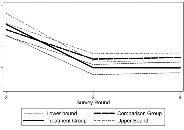
The drop-off in attendance as implied by the steepness of the slopes shown in Figure 2 is larger for girls in the comparison districts than it is for girls in the treatment districts. As a placebo test, I repeat the exercise for girls’ enrollment in private schools (Figure 3). I find that there is no differential change in the attendance probability for girls in private schools. This is to be expected if the stipend program did not induce parents to switch from private to public schools. There has been no evidence to date of this having occurred. Taken together, Figures 2 and 3 suggest that over time girls who reside in the treatment district and are in the typical age-range for grades 6 through 8 seem to be attending public schools at a higher rate over time than similar girls in the comparison district.
I next use the data from the school surveys conducted by the LEAPS team to plot the percent of all students who drop out over the course of the LEAPS survey. Figure 4 shows the dropout rate for children in public schools. Over the course of the survey period the drop-out rate from public schools in the comparison districts is fairly stable at 6 percent. In contrast, the drop-out rate clearly falls over time in the treatment district from 5 percent (at which point it is statistically indistinguishable from the dropout rate in the comparison districts) to 2 percent (which is statistically different). Again, to provide evidence that the changes in public schools are likely the results of the stipend program, I also plot dropout rates for private schools (Figure 5). There is no difference between treatment and comparison districts in the level or trend in drop-out rates from private schools. The confidence intervals for private schools in the treatment and comparison districts overlap everywhere. Figures 4 and 5 together suggest that there is no difference at baseline in dropout rates between public schools in the treatment and comparison
districts. They also suggest that a difference in drop-out rates emerges over time for public schools and that a similar difference is not present in the data on private schools.
Both of the preceding pieces of evidence suggest that the female student stipend program appears to be having an effect in the treatment district relative to the comparison districts.
Admittedly, each piece has its own limitations and these results do not constitute a
comprehensive evaluation of the effectiveness of the program as a whole. They do, however, provide some evidence regarding the channels through which the program appears to be
operating – a slowdown in the attrition rate from public schools for girls in the treatment district. In order to more convincingly establish that this is the case, I conduct a more stringent test by comparing the difference in outcomes between individuals and in family at time in the treatment district with this difference for families in the comparison district. I estimate the following model:
(1)
which assumes that the error term can be decomposed as follows:
(1a) The term represents the effects of unobservables that vary across families but are constant for individuals within the same family and terms are independently and identically distributed. I define two indicator functions: which denotes whether or not individual is a female and
which denotes whether or not family resides in the treatment district. Intuitively, I take differences between a girl and a boy ( and ) in the same family and compare how this difference evolves over time for families in the treatment district relative to how it evolves for families in the comparison districts. I am able to do this for three post-program periods.
I implement this as follows. I remove from the LEAPS sample households where all the children are boys (106 households) or households where all the children are girls (75
households). These households are not informative for the comparison performed here. I then enter dummy variables for the interaction between households and years. Standard errors are clustered by individual to allow for the correlation of observations from the same individuals over time. The coefficients of interest are the interactions between gender of the child, whether or not the family is in the treatment district and whether or not the data are from post-program rounds , . In Table 3, I report the results from this within family difference-in-differences estimator. As suggested above, the point estimates are positive and increase over time from practically (and statistically) no difference in the first post-program year to a one percentage point difference and then a statistically significant three percentage point difference over the course of the LEAPS survey.
The evidence in Table 3 suggests that by round 4 of the LEAPS survey, female children in the treatment district are roughly 3 percentage points more likely to be attending public schools than their male siblings relative to those in the comparison districts. Models that control for characteristics of the individual are similar and insensitive to choice of specification used.11 VI.Evidence of program impact on household time allocation
Having provided several pieces of evidence which suggest that the stipend program influenced girls’ enrollment, I turn to the main question posed at the outset of this paper: Do households reallocate time use when conditional cash transfers are provided to them? To answer it, I employ a standard difference-in-difference approach, briefly explained below.
Consider the stylized example depicted in Figure 6. Data are available on an outcome ( ) for households from two groups – those eligible for treatment ( ) and those ineligible for
11
treatment . The vertical dashed line at time t represents the implementation of the
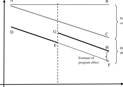
program. Consequently t-1 is the baseline period and t+1 is the post-program period. Outcomes for two groups are shown: the comparison group (solid grey line) and the treated group (solid black line). The dotted line AB represents no change in the outcome of interest over time. The solid grey line AC represents the evolution of the outcome of the comparison group over time. Consequently, the distance BC is the natural trend in the outcome over time that would exist in the absence of any program. Without such information from a comparison group, the effect of the program would be overstated. Likewise, the line DEF shows how the outcome for the treated group would have evolved in the absence of the program.12 The difference between the two groups at baseline (the distance AD) is assumed to have persisted (the distance CF is drawn to equal the distance AD). However, the implementation of policy causes the outcome for the treated group to evolve differently. Consequently, the outcome for the treated group follows the path GH after the program is implemented. Using the difference-in-differences methodology allows the decomposition of outcomes over time into a part due to a natural trend over time (BC), a part due to pre-existing differences between the two groups (CF) and the part that is due to the program (FH).
The data reveal that in districts where there is no stipend program, on average parents are more likely to send their children to school. When these children are at school, they do not help around the house. Consequently any housework is done by the mother or siblings who are old enough to help out and not in school. As they grow older and reach the end of class five – the end of the primary cycle in Pakistan – these children typically drop out of school. Once they have done so they are unlikely to return to school. Such children are again in a position to help
12
The segment DE is known and the segment EF is a counterfactual assumption. The choice of a positively trending outcome in this figure is completely arbitrary and has no bearing on the intuition.
around the house. Thus the mothers of school-going children in districts with no stipend program provide a picture of the typical pattern of time use in the absence of the program. In the context of Figure 6, they provide the information necessary to draw the line AC. While their children are in school, they likely report the following pattern of time use: large amounts of housework combined with low amounts of time spent on children’s needs. As their children drop out the mothers in non-stipend districts likely report smaller amounts of housework and larger amounts of time spent on children’s needs. At some level this is tautological. The children are now in the home and the mother must spend some time on their needs. Since she only has twenty-four hours in the day she must report spending less time in other activities.
By contrast in the districts where the stipend program is available, children who are in school are likely to delay dropping out and children who would otherwise not have gone might start going to school. Thus their mothers are unlikely to be able to adjust their hours by
devolving housework to children who have dropped out. Nor would they need to spend more time on children’s needs since these children are more likely to be in school or at least in school longer. Consequently, these individuals provide the information necessary to draw lines DE and GH.
a. Descriptive comparisons
In Table 4, I apply this methodology and report sample means of the outcomes of interest for eligible households in both treatment and comparison group districts over time. The four outcomes are the amount of time spent on (i) housework, (ii) paid work, (iii) looking after children’s needs and (iv) sleep. The survey defines housework as time spent on cooking, cleaning, looking after livestock, performing unpaid non-agricultural family work outside the house and working on one’s own farm. Paid work is defined as time spent on farm work, looking
after livestock, time in self-employed work, household industry (such as embroidery), or
working as a salaried worker. Children’s needs are described as bathing or feeding.13 Looking at the unadjusted difference-in-differences estimate of the effect of the program, I find that there are differences in the time use patterns of eligible households from the treatment district relative to those in the comparison districts. Specifically, comparing the time use data from round 1 (the baseline) with the data from round 3 (one year after the program began), mothers from stipend-eligible households in the treatment district report spending roughly 82 additional minutes per typical school day on housework compared to mothers from eligible households in the
comparison districts. Similarly they report spending 30 fewer minutes on paid work, 78 fewer minutes on children’s needs and report getting slightly approximately 20 fewer minutes of sleep relative to those in the comparison districts.
When I compare the baseline data to that from round 4, I find that the unadjusted effect of the program on time spent on housework, paid work and children’s needs is qualitatively and quantitatively unchanged and that the direction of the effect stays the same –housework goes up and paid work and time spent on children’s needs goes down. The effect on sleep stays
practically small and is now positive.14 b. Methodology
In order to see if these trends are robust to the inclusion of controls, I estimate the following empirical specification:
13
The questionnaire seems to imply that surveyors suggested the following definition of children’s needs to the respondent “bathing/feeding etc.” Looking after child’s studies and sickness are separate categories.
14
When I examine the additional activities respondents report, I find that the net change in activities balances out. For instance, if the unadjusted difference in difference suggests that mothers worked 2 more hours in the house and reduced their paid work and the time they spend on children’s needs by 3 hours, the remaining difference of 1 hour is recouped across the remaining activities.
(2) Where is the time spent by mother at time in a given activity (housework, paid work, child needs or sleep), the vector is a set of her observable characteristics, the terms and are indicator variables for rounds 3 and 4 of the LEAPS survey. The coefficient captures the effect of the program one year after program implementation and the coefficient captures the effect of the program two years after program implementation. Given that I estimate this relationship using the subsample of eligible households in both treatment and control
districts, these two coefficients represent the intent-to-treat effect of the program. The term reflects an individual fixed effect and incorporates the influence of time-invariant regressors – measured and unmeasured – on mother’s time use.15
c. Results
In columns 1 and 2 of Table 5, I first examine the extensive margin – whether the fraction of mother’s who report participating in housework changes differentially across treatment and comparison samples. I compare mothers from households with eligible girls in the treatment district with mothers from households with eligible girls in the comparison districts. Column 1 ignores the availability of panel data and presents results from pooled ordinary least squares (OLS) regression. Column 2 allows for a fixed effect at the level of the mother – the unit of analysis in this table. In both cases there is no difference over time in the fraction of mothers who report spending time in household work when one compares households with eligible children in the treatment district and the comparison districts. The mean level of participation in housework at baseline is 97 percent. This suggests that any differences in the intensive margin –
15
This fixed effects difference-in-differences estimator is an improvement over the difference estimator employed in Skoufias and Parker (2001) since I am now able to adjust for pre-program differences directly and am able to examine if the effect persists.
the amount of housework reported – are not the result of survey respondents becoming better at reporting their time use or being more likely to report housework.
In columns 3 – 7, I find evidence to suggest that relative to the mothers of those who are ineligible to receive the stipend program, the mothers of those who are eligible experience an increase in the amount of time they spend on housework. Columns 3 and 4 contain no controls and report estimates from pooled OLS and fixed effects regressions respectively. In columns 5 – 7, I introduce three sets of sequentially augmented controls– basic, extended and full. The basic specification controls for differences in household size and composition with a set of indicator variables for the number and gender of household members of various ages. I include separate controls for the number of men, the number of women, the number of teen boys (ages 13 to 17), teen girls, preteen boys (ages 5 to 12) and preteen girls as well as the number of male and female infants (those children under the age of 5).
The extended set of controls adds to the household size and composition variables a series of indicator variables that measure the current and relative wealth of the respondents. I include an index of household wealth – which is the score of the first principal component of an index derived from whether or not a household owns items from a list of assets.16 The LEAPS survey asks households to rate their wealth relative to five years ago as well as their harvest relative to one year ago. Responses to both these questions were categorical and as such indicator variables were included to capture their inherent non-linearity. The full set of controls adds a set of indicators for mother and father’s age as well as indicator variables for quarter of interview. If some seasonal differences confound the intent to treat effects of the program, controlling for quarter of interview addresses this issue.
16
Households were asked if they owned any of the following: beds, tables, chairs, fans, sewing machines, air coolers, air conditioners, refrigerators, radio cassette players, TVs, VCRs, and watches. Reponses were combined using principal components analysis. The first principal component is a standard normal variable.
At baseline, the average mother of a stipend-eligible child in a treatment district
household in the LEAPS sample reports spending 516 minutes on housework on a typical school day. Column 7 – the specification with the full set of controls – suggests that the availability of the stipend program increases the amount of time mothers in stipend-eligible households spend on housework by approximately 100 minutes (1 hour and 40 minutes). This point estimate corresponds to an effect of roughly 19 percent when compared with mothers in stipend ineligible households.17 This increase is the same order of magnitude regardless of whether I look at round 3 of the LEAPS survey or round 4. I fail to reject the null hypothesis that the two coefficients are equal. Together this is evidence that the effect of the stipend program persists from one year to the next.
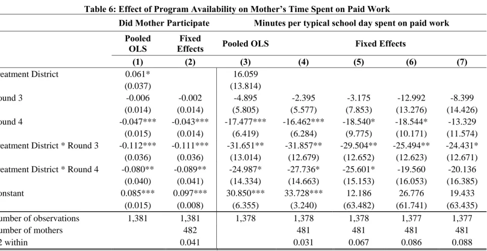
Table 6 reports the results from a similar exercise conducted on mother’s time spent on paid work. In contrast to the results on housework, I find no appreciable change in the amount of time reported on paid work. I do find evidence of a substantial difference on the extensive margin however: mothers from stipend-eligible households in the treatment district are
substantially more likely to stop reporting time spent on paid work over time when compared to mothers from similar households in the comparison districts.
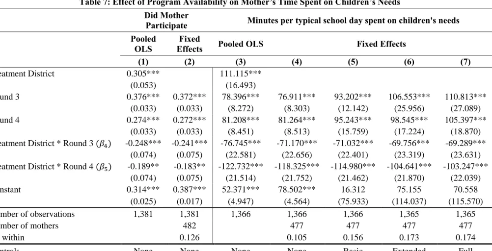
While housework and paid work are typically the outcomes of interest in most studies, Table 7 exploits the availability of detailed data in the LEAPS survey and focuses on time spent looking after children’s needs. As in the case of paid work, there is a substantial reduction in the fraction of mothers reporting time spent on children’s needs in the treatment district relative to the comparison districts. On average, over time mothers report spending roughly 1 hour less on this type of activity if they live in the treatment district than if they live in the comparison districts.
17
Table 8 shows that there is no statistical difference between treatment and control group households in their reported amount of sleep. The point estimates are practically small and statistically indistinguishable from zero. Thus while this would seem to be one margin on which mother’s could adjust they do not.
The evidence presented thus far suggests that mothers of stipend-eligible children in the stipend district have different trajectories of time use than mothers of similar children in the comparison districts. The evidence suggests that mothers spend more time on housework and less time on children’s needs. I find no evidence of changes in the amount of time respondents sleep or participate in paid work. The inclusion of controls does not explain away the effect of the program – which in the preferred specification is an increase of about 100 minutes per typical school day of housework and a reduction of 70 minutes of time spent on children’s needs.
VII. Robustness Checks
One critique that could reasonably be leveled at the analysis presented thus far is the fact that I agglomerate two districts into one comparison group. Administrative data presented in figure 7, shows total female enrollment in grades 6-8 (panel a) and all grades (panel b) for all three districts of the LEAPS data. This figure suggests that Attock is a more appropriate comparison group if baseline enrollment is taken as the yardstick for comparability.
Consequently in Tables 9 and 10, I report the results of the full specification using each district, Faisalabad and Attock respectively, separately as a comparison for the stipend district – Rahim Yar Khan.18 These specifications include all control variables. I find that the results are qualitatively and quantitatively unchanged. Mothers of stipend eligible children in Rahim Yar Khan report roughly two more hours of housework and roughly one hour and forty minutes less
18
I also examine if there is any evidence of systematic differences within the treatment district. I compare the characteristics of households with only boys in the eligible age range with those of households with girls in the eligible age range. I find no statistical evidence of any differences between these two groups.
of time spent on children’s needs when compared with mothers of stipend-eligible children in Attock. There is little difference over time in either paid work or sleep time. An alternative means of interpreting the point estimates is to compare their magnitude to baseline averages for the sample. As reported in Table 9, the mean amount of time spent on housework reported at baseline is 516 minutes per typical school day. Consequently, the point estimate suggests that program availability is associated with a 23 percent increase in housework.19
As a final check, I am particularly liberal in the removal of outlying observations. I re-run the analysis eliminating any households that in addition to providing outlying data on their total time use also provided outlying observations on a particular activity. Thus if a household’s responses account for 24 hours correctly, but the household reports spending 18 hours a day on one activity – for example housework (a value that is extreme relative to the rest of the
distribution in the data), I remove that household from the analysis. I do so for each activity considered in the paper. I find this does not influence the size or direction of the effects.
The evidence thus far suggests that households of stipend eligible children in the treatment district have different time use profiles over time than similar households in the districts where there is no such program. The skeptical reader might still be concerned that what is being referred to here as an effect of the stipend program is in fact the result of pre-program differences stemming from differences in the composition of the households at baseline. If that were true, the effects of household composition should persist and I should see no difference over time in the time-use patterns of households in the treatment and comparison districts.
At baseline, households of eligible children in the treatment district have more boys and fewer girls (ages 5 – 17). In addition they also have more infant children (under 5). From the
19
An alternative way of interpreting the output is to consider what fraction of time in the day is allocated to each activity. Such as analysis says that the share of the day devoted to housework increases by 0.09 and that devoted to children’s needs decreases by 0.07. There is no difference in shares of the day devoted to sleep and paid work
point of view of being able to divest responsibility to their daughters, the mothers in these
households would then appear to be over-burdened (they have “too many” boys who are not very productive around the house) and under-staffed (they have “too few” girls who can help out). When the stipend program begins operating and these girls start to attend school, the mothers in the treatment district have more to do as the girls have less time to help out. Another
consequence of girls going to school is that the mother has fewer children around the house on whose needs a mother can report spending time on a typical school day. Such a situation should persist as children age and households do not respond by differentially changing their fertility. In analyses not reported in this paper, I investigate if there is any evidence of differential growth in household size between the treatment and comparison households and find no such evidence. VIII. Discussion
Relative to mothers in households that were ineligible to receive the program, mothers in eligible households increase the amount of time that they report on housework by about two hours per typical school day. Considering that the typical eligible school girl reports spending four hours a day in school, I account for roughly half of the time a girl is away. This is likely due to two complementary reasons – the fact that an adult woman is more productive per unit time in the kinds of activities that fall under housework and the fact that not all the girls’ time at home was being spent in housework to begin with.
The data suggest that a gender-targeted conditional cash transfer program produces substantial changes in household time allocation. Such changes are not the goal of this program but must inevitably occur when it and similar programs are successful. Are such unintended consequences necessarily harmful from a societal point of view? In my opinion, the answer is a qualified no. The qualification stems from the fact that what is missing in the present analysis is
similarly detailed household data not only from the three districts analyzed here but also from all the districts in the province.20
In their haste to adopt a type of program that has been successful elsewhere,
policymakers incorporated some elements (the conditionality and relative size of the transfer) but changed others (the targeting based on gender). If the literature on program evaluation has taught us anything it is that generalizing from one setting to another is at best optimistic and at worst an exercise doomed to failure. This seems particularly true of evaluations of programs in developing countries where program design and implementation frequently are found to diverge.
Consequently policymakers in these countries should be more careful to incorporate data collection at baseline and at follow-up to ensure that context-specific evaluations are possible.
The analysis presented here and existing evidence on the effects of the program suggest that it is successful in sending girls to school. A substantial body of evidence exists on the benefits to society of educating women.21 The children of more educated mothers have better educational and health outcomes. Such evidence alone should justify the continuation of this gender-targeted stipend program – with obvious attention being paid to capacity constraints that are known to emerge in schools and education systems. However, an examination of data from the PSLM suggests another channel through which society could benefit from such programs. There is a stark correlation between regional levels of maternal literacy and the sex ratios of children within households (Figure 8). Specifically it appears that in regions with lower levels of literacy there is a substantially higher ratio of boys to girls. If we are to take this correlation seriously then it appears that in the long-run, the stipend program has the potential to impart
far-
20
The analysis presented here was made possible by the fortuitous timing with which researchers fielded a survey and not the result of an attempt by policymakers to adequately monitor and evaluate the program.
21
See for instance the arguments in Schultz, 2001 on the need for governments the world over to invest more in girls’ education and the evidence in Andrabi et. al., 2007 on how educated girls transition from being students today to teachers tomorrow in the Pakistani districts studied in the present paper.
reaching benefits to society – it could well correct this imbalance. As such, the program should not be abandoned in the name of expediency as has recently been the fate of policies in Pakistan.
Table 1
Country (Program) Condition Size of transfer (US$/year)* Eligibility Stipend Programs for all children
Mexico (Progresa / Oportunidades) Min 85% attendance monthly and annually Primary School: 8 - 17 (varies by grade)
Children from poor households ages 8-18 enrolled in primary, secondary or upper secondary school
Secondary School: 25 - 32 (varies by grade and gender) Allowances for school materials
Nicaragua (RPS) 85 % attendance per month. (No more than 3 unexcused absences per month.)
112 per household Children aged 7 – 13 who have not completed grade 1- 4.
4.75 per child to schools
Honduras (PRAF II) Max absence of 7 days in 3 month period
58 per child Children from poor households ages 6-12 who have not yet completed grade 4 4000 per school
Turkey (SSF) Min 85% attendance
85.5 for first child Children from poor households ages 6 and over enrolled in grades 1-11
72 for second child 58.5 for each subsequent child
Colombia (FA) 80% attendance in a two-month cycle
Primary School: 54 Children from poor households ages 7-17 enrolled in school (grades 2-11)
Secondary School: 81
Stipend Programs for Girls only
Cambodia (JFPR) Max: 9 days in the year "with good reason"
45 Female student enrolled in lower
secondary school who maintains a passing grade
Pakistan (FSSP) 80% attendance 30 per child Female student enrolled in grades 6 - 8 in a government school
Bangladesh (FSSAP) Min: 75 percent of school days
10-35 (varies by grade and type of school (government or non-government)
Female student enrolled in secondary school in rural areas who attains 45 percent of class-level test scores and remains unmarried
* Monthly amounts converted to annual under the assumption that a typical school year lasts 9 months. Figures for Bangladesh computed using 1996 exchange rate (year of program start). Figures for Pakistan computed using 2004 exchange rate (year of program start).
Table 2
Literacy Ratio (Population age 10 and over)
Districts Census 1998 1 Rawalpindi 71 2 Lahore 65 3 Jhelum 64 4 Gujrat 62 5 Sialkot 59 6 Chakwal 57 7 Gujranwala 57 8 Narowal 53 9 Faisalabad 52
10 Toba Tek Singh 51
11 Attock 49 12 Mandhi Bahauddin 47 13 Sargodha 46 14 Sahiwal 44 15 Sheikhupura 44 16 Mianwali 43 17 Multan 43 18 Hafizabad 41 19 Khushab 41 20 Khanewal 40 21 Layyah 39 22 Okara 38 23 Jhang 37 24 Vehari 37 25 Kasur 36 26 Bahawalnagar 35 27 Pakpattan 35 28 Bahawalpur 35 29 Bhakkar 34
30 Rahim Yar Khan 33
31 Dera Ghazi Khan 31
32 Lodhran 30
33 Muzaffar Garh 29
34 Rajanpur 21
The dotted line represents the literacy cutoff used by the government in determining program eligibility at the district level. The one highlighted district below the line is the treatment district in this analysis. Districts above the dotted line were deemed ineligible. The two districts in bold are control group districts in the present analysis.
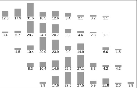
Figure 1: The Age-Grade Distribution in post-primary grades
Each row is a different post-primary grade. Each histogram is the percent of class enrollment that belongs to a particular age category. Thus the figure suggests that 31.6 percent of all the girls in class 6 in the rural areas of Attock, Faisalabad (comparison) and Rahim Yar Khan (treatment) are 12 years old. Similarly 52.8 percent (28.7+24.1) of the enrollment in class 7 is made up of girls who are 12 and 13 years old.
12.6 17.9 31.6 10.5 12.6 8.4 2.1 3.2 1.1 3.4 5.7 28.7 24.1 20.7 9.2 4.6 2.3 1.1 4.5 10.4 29.9 23.9 9.0 14.9 6.0 1.5 8.3 10.4 14.6 22.9 27.1 8.3 4.2 4.2 3.9 17.6 27.5 27.5 5.9 11.8 2.0 3.9 Class 10 Class 9 Class 8 Class 7 Class 6 Current class 10 11 12 13 14 15 16 17 18 19 20+ Age (Years)
Source: Pakistan Social and Living Standards Measurement Survey 2004-2005
Girls in rural Attock, Faisalabad and Rahim Yar Khan
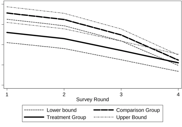
Figure 2: Probability of attending a public school
Note: Thick solid line represents sample average for girls in the treatment district. Thick dashed line represents sample average for girls in the comparison districts. Confidence intervals are marked using small dashes (lower bound) and lines that alternate dashes and dots (upper bound). The mean enrollment levels are statistically different in rounds 1 and 2. The fall-off in attendance is steeper in the comparison districts than in the treatment districts. The probability of attending public school at baseline (round 1) is 0.36 for girls in the treatment district and 0.46 for girls in the comparison districts.
.1
.2
.3
.4
.5
Probability of attending public school
1 2 3 4
Survey Round
Lower bound Comparison Group
Treatment Group Upper Bound
Girls 10-14 years old at baseline
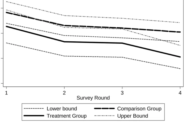
Figure 3: Probability of attending a private school
Note: Thick solid line represents sample average for girls in the treatment district. Thick dashed line represents sample average for girls in the comparison districts. Confidence intervals are marked using small dashes (lower bound) and lines that alternate dashes and dots (upper bound). The mean enrollment levels are statistically indistinguishable from each other in rounds 1,2 and 3. The probability of attending a private school at baseline (round 1) is 0.11 for girls in the treatment district and 0.14 for girls in the comparison districts.
0
.05
.1
.15
Probability of attending private school
1 2 3 4
Survey Round
Lower bound Comparison Group
Treatment Group Upper Bound
Girls 10-14 years old at baseline
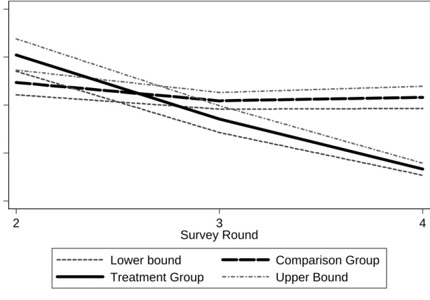
Figure 4: Dropout rate from public schools
Note: Thick solid line represents sample average for the treatment district. Thick dashed line represents sample average for the comparison districts. Confidence intervals are marked using small dashes (lower bound) and lines that alternate dashes and dots (upper bound). Data exist for all four rounds. The y-axis is the percentage of children dropping out. The mean at baseline for the treatment district is 0.061 and the mean at baseline for the comparison districts is 0.049.
0
.02
.04
.06
.08
Percentage of students dropping out
2 3 4
Survey Round
Lower bound Comparison Group
Treatment Group Upper Bound
Public schools
Figure 5: Dropout rate from private schools
Note: Thick solid line represents sample average for the treatment district. Thick dashed line represents sample average for the comparison districts. Confidence intervals are marked using small dashes (lower bound) and lines that alternate dashes and dots (upper bound). Data exist for all four rounds. The y-axis is the percentage of children dropping out. The mean at round 2 for the treatment district is 0.062 and the mean at round 2 for the comparison districts is 0.056.
0
.02
.04
.06
.08
Percentage of students dropping out
2 3 4
Survey Round
Lower bound Comparison Group
Treatment Group Upper Bound
All other schools
Table 3: Differences between girls and their male siblings
Does child attend public school
(1) (2)
Is Child Female -0.006 0.011
(0.009) (0.007)
Is Child Female * Treatment District -0.080*** -0.080***
(0.018) (0.016) Is Child Female * Treatment District * Year 2 0.002 0.003
(0.013) (0.013) Is Child Female * Treatment District * Year 3 0.016 0.012
(0.016) (0.015) Is Child Female * Treatment District * Year 4 0.035** 0.028*
(0.017) (0.017) Constant 0.270*** 0.021 (0.005) (0.014) Number of observations 36,544 36,133 Number of individuals 9,136 9,136 Adjusted R2 0.174 0.413
Family * Year Dummies Y Y
Controls N Y
note: *** p<0.01, ** p<0.05, * p<0.1. Column 2 includes a series of indicator variables for age of the child. Standard errors are robust to heteroskedasticity and are clustered to allow for repeated observations on the same child.
Figure 6: Stylized Description of methodology
Vertical dashed line at time t represents the implementation of the program. Consequently t-1 is the baseline period and t+1 is the post-program period. Outcomes for two groups are shown: the comparison group (solid grey line) and the treated group (solid black line). The dotted line AB represents no change in the outcome of interest over time. The solid grey line AC represents the evolution of the outcome of the comparison group over time. Consequently, the distance BC is the natural trend in the outcome over time that would exist in the absence of any program. The line DEF shows how the outcome for the treated group would have evolved in the absence of the program. The difference between the two groups at baseline (the distance AD) would have persisted (the distance CF is drawn to equal the distance AD). However, the implementation of policy causes the outcome for the treated group to evolve differently. Consequently, the outcome for the treated group follows the path GH after the program is implemented. Using the
difference-in-differences methodology allows the decomposition of outcomes over time into the a part due to a natural trend over time (BC), a part due to pre-existing differences between the two groups (CF) and the part that is due to the program (FH).
t-1 t Y1, Y0 Time t+1 Estimate of program effect F A B E G
Difference between groups in the absence of the program
H C D
Natural trend in outcome over time
Table 4: Unadjusted estimates
Minutes per typical school day spent by mother on :
All House Work All Paid Work Children's Needs Sleep
Treated Comparison Δ Treated Comparison Δ Treated Comparison Δ Treated Comparison Δ
Round 1 Mean 528 603 45 29 166 55 593 579 SD 231 207 126 116 174 93 201 137 N 128 385 Round 3 Mean 475 468 82 9 23 -30 171 139 -78 643 651 -21 SD 189 184 65 95 146 134 125 117 N 129 397 Round 4 Mean 523 506 92 8 13 -22 128 134 -117 660 635 11 SD 148 193 52 75 102 136 105 117 N 127 374
Let T denote Treated and C denote Comparison. Then for each outcome and round , ∆ . Treated households are from Rahim Yar Khan district and have at least one child who is eligible for receipt of the stipend. Comparison households are pooled from the two
comparison group districts – Attock and Faisalabad – and have at least one child who would be eligible if the stipend program existed in those districts. The changes in sample size from one round to the next reflect the net effect of observations lost due to attrition from the survey and those lost due to missing or outlying data. Housework is defined as including unpaid work on the family farm, looking after livestock, cooking, cleaning and unpaid non-agricultural work outside the home. Paid work is work for pay on a farm, looking after livestock, working in household industry, working as a laborer or being self-employed. Children's needs are defined as bathing and feeding. Each outcome is reported as minutes spent on a given activity per typical school day. Housework changes are driven by changes in minutes of cooking. Paid work changes are virtually all noise as very few of the mothers in these households work for pay.
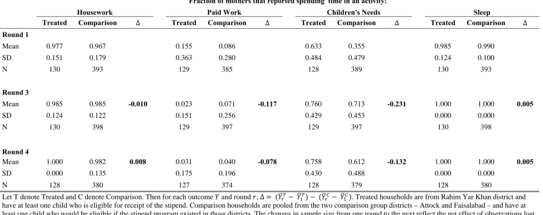
Table 4a: Unadjusted estimates
Fraction of mothers that reported spending time in an activity:
Housework Paid Work Children's Needs Sleep
Treated Comparison ∆ Treated Comparison ∆ Treated Comparison ∆ Treated Comparison ∆
Round 1 Mean 0.977 0.967 0.155 0.086 0.633 0.355 0.985 0.990 SD 0.151 0.179 0.363 0.280 0.484 0.479 0.124 0.100 N 130 393 129 385 128 389 130 393 Round 3 Mean 0.985 0.985 -0.010 0.023 0.071 -0.117 0.760 0.713 -0.231 1.000 1.000 0.005 SD 0.124 0.122 0.151 0.256 0.429 0.453 0.000 0.000 N 130 398 129 397 129 397 130 398 Round 4 Mean 1.000 0.982 0.008 0.031 0.040 -0.078 0.758 0.612 -0.132 1.000 1.000 0.005 SD 0.000 0.135 0.175 0.196 0.430 0.488 0.000 0.000 N 128 380 127 374 128 379 128 380
Let T denote Treated and C denote Comparison. Then for each outcome and round , ∆ . Treated households are from Rahim Yar Khan district and have at least one child who is eligible for receipt of the stipend. Comparison households are pooled from the two comparison group districts – Attock and Faisalabad – and have at least one child who would be eligible if the stipend program existed in those districts. The changes in sample size from one round to the next reflect the net effect of observations lost due to attrition from the survey and those lost due to missing or outlying data. Housework is defined as including unpaid work on the family farm, looking after livestock, cooking, cleaning and unpaid non-agricultural work outside the home. Paid work is work for pay on a farm, looking after livestock, working in household industry, working as a laborer or being self-employed. Children's needs are defined as bathing and feeding. Each outcome is reported as a binary variable equal to one if minutes spent on a given activity per typical school day were reported.
Table 5: Effect of Program Availability on Mother’s Time Spent on Housework
Minutes per typical school day mother spent on housework
Pooled OLS Fixed Effects
(1) (2) (3) (4) (5) Treatment District -89.942*** (25.073) Round 3 -133.901*** -133.743*** -157.467*** -176.368*** -197.911*** (13.073) (13.166) (18.160) (33.311) (35.644) Round 4 -103.437*** -106.081*** -135.484*** -139.177*** -161.650*** (14.735) (14.643) (23.850) (26.232) (28.721)
Treatment District * Round 3 111.537*** 111.051*** 106.291*** 107.095*** 101.943***
(27.268) (27.024) (27.668) (29.028) (29.912)
Treatment District * Round 4 116.609*** 117.421*** 106.512*** 98.441*** 100.043***
(28.902) (29.384) (28.564) (29.117) (29.899) Constant 606.215*** 585.636*** 672.595*** 665.762*** 700.157*** (11.083) (7.038) (103.884) (140.299) (137.522) Number of observations 1,381 1,381 1,381 1,380 1,380 Number of mothers 482 482 482 482 R2 within 0.109 0.148 0.160 0.165
Controls None None Basic Extended Full
p-value of F-test of : 0.9928 0.7210 0.9390
note: *** p<0.01, ** p<0.05, * p<0.1.The mean of the dependent variable for columns 1 and 2 is 0.9688 at baseline. For columns 3 – 7 the mean of the dependent variable at baseline is 516 minutes/typical school day. Basic controls:a series of indicator variables that fully describe the composition of the household by age and gender. For example: an indicator for each number of adult men, women, teenage boys, teenage girls, pre-teen girls, pre-teen boys as well as infant boys and girls. Extended: In addition to basic
specification includes age of mother and father as well as indicators for whether this information is missing. Includes an asset index measured as the first principal component of a list of 16 assets over all rounds of the data. Also includes a series of indicators for wealth status of household as measured by wealth relative to five years ago and harvest relative to last year. Full: In addition to extended controls a series of indicator variables for quarter in which household was interviewed. Round 3 is the first post-program year for which LEAPS data on this outcome is available. Heteroskedasticity-robust standard errors in parentheses. Standard errors adjust for clustering at the mother level.
Table 6: Effect of Program Availability on Mother’s Time Spent on Paid Work
Did Mother Participate Minutes per typical school day spent on paid work
Pooled OLS
Fixed
Effects Pooled OLS Fixed Effects
(1) (2) (3) (4) (5) (6) (7) Treatment District 0.061* 16.059 (0.037) (13.814) Round 3 -0.006 -0.002 -4.895 -2.395 -3.175 -12.992 -8.399 (0.014) (0.014) (5.805) (5.577) (7.853) (13.276) (14.426) Round 4 -0.047*** -0.043*** -17.477*** -16.462*** -18.540* -18.544* -13.329 (0.015) (0.014) (6.419) (6.284) (9.775) (10.171) (11.574) Treatment District * Round 3 -0.112*** -0.111*** -31.651** -31.857** -29.504** -25.494** -24.431*
(0.036) (0.036) (13.014) (12.679) (12.652) (12.623) (12.671) Treatment District * Round 4 -0.080** -0.089** -24.987* -27.736* -25.601* -19.560 -20.136
(0.040) (0.041) (14.334) (14.663) (15.153) (16.053) (16.385) Constant 0.085*** 0.097*** 30.850*** 33.728*** 12.186 26.776 19.433 (0.015) (0.008) (6.355) (3.240) (63.482) (61.741) (63.435) Number of observations 1,381 1,381 1,378 1,378 1,378 1,377 1,377 Number of mothers 482 481 481 481 481 R2 within 0.041 0.031 0.067 0.086 0.088
Controls None None None None Basic Extended Full
note: *** p<0.01, ** p<0.05, * p<0.1. The mean of the dependent variable for columns 1 and 2 is 0.1014. The mean of the dependent variable for columns 3 – 7 at baseline is 47 minutes/typical school day. Basic controls: a series of indicator variables that fully describe the composition of the household by age and gender. For example: an indicator for each number of adult men, women, teenage boys, teenage girls, pre-teen girls, pre-teen boys as well as infant boys and girls. Extended: In addition to basic specification includes age of mother and father as well as indicators for whether this information is missing. Includes an asset index measured as the first principal component of a list of 16 assets over all rounds of the data. Also includes a series of indicators for wealth status of household as measured by wealth relative to five years ago and harvest relative to last year. Full: In addition to extended controls a series of indicator variables for quarter in which household was interviewed. Round 3 is the first post-program year for which LEAPS data on this outcome is available. Heteroskedasticity-robust standard errors in parentheses. Standard errors adjust for clustering at the mother level.
Table 7: Effect of Program Availability on Mother’s Time Spent on Children’s Needs
Did Mother Participate Minutes per typical school day spent on children's needs
Pooled OLS
Fixed
Effects Pooled OLS Fixed Effects
(1) (2) (3) (4) (5) (6) (7) Treatment District 0.305*** 111.115*** (0.053) (16.493) Round 3 0.376*** 0.372*** 78.396*** 76.911*** 93.202*** 106.553*** 110.813*** (0.033) (0.033) (8.272) (8.303) (12.142) (25.956) (27.089) Round 4 0.274*** 0.272*** 81.208*** 81.264*** 95.243*** 98.545*** 105.397*** (0.033) (0.033) (8.451) (8.513) (15.759) (17.224) (18.870)
Treatment District * Round 3 -0.248*** -0.241*** -76.745*** -71.170*** -71.032*** -69.756*** -69.289*** (0.074) (0.075) (22.581) (22.656) (22.401) (23.319) (23.631) Treatment District * Round 4 -0.189** -0.183** -122.732*** -118.325*** -114.980*** -104.641*** -103.247***
(0.074) (0.075) (21.514) (21.752) (21.462) (21.870) (22.039) Constant 0.314*** 0.387*** 52.371*** 78.502*** 16.312 75.155 70.558 (0.025) (0.017) (4.947) (4.564) (75.933) (114.037) (115.570) Number of observations 1,381 1,381 1,366 1,366 1,366 1,365 1,365 Number of mothers 482 477 477 477 477 R2 within 0.126 0.105 0.156 0.173 0.174
Controls None None None None Basic Extended Full
p-value of F-test of : 0.0205 0.0677 0.0791
note: *** p<0.01, ** p<0.05, * p<0.1. For columns 1 and 2, the mean of the dependent variable at baseline is 0.4191. For columns 3 – 7 the mean of the dependent variable is 168 minutes/typical school day. Basic controls: a series of indicator variables that fully describe the composition of the household by age and gender. For example: an indicator for each number of adult men, women, teenage boys, teenage girls, pre-teen girls, pre-teen boys as well as infant boys and girls. Extended: In addition to basic specification includes age of mother and father as well as indicators for whether this information is missing. Includes an asset index measured as the first principal component of a list of 16 assets over all rounds of the data. Also includes a series of indicators for wealth status of household as measured by wealth relative to five years ago and harvest relative to last year. Full: In addition to extended controls a series of indicator variables for quarter in which household was interviewed. Round 3 is the first post-program year for which LEAPS data on this outcome is available. Heteroskedasticity-robust standard errors in parentheses. Standard errors adjust for clustering at the mother level.
Table 8: Effect of Program Availability on Mother’s Time Spent on Sleep
Minutes per typical school day spent on sleep
Pooled OLS Fixed Effects
(1) (2) (3) (4) (5) Treatment District -15.331 (17.812) Round 3 71.102*** 70.223*** 70.896*** 23.815 20.666 (9.029) (9.146) (14.098) (23.508) (24.424) Round 4 57.401*** 58.115*** 60.004*** 59.234*** 52.211*** (9.176) (9.249) (17.098) (17.805) (19.656)
Treatment District * Round 3 0.917 -0.992 2.476 -4.202 -4.280
(18.940) (19.137) (19.567) (20.316) (20.533)
Treatment District * Round 4 37.231* 35.758* 40.379** 28.752 26.205
(19.580) (19.658) (20.241) (20.947) (21.002) Constant 581.581*** 578.394*** 576.294*** 496.830*** 498.930*** (6.964) (4.781) (78.223) (84.996) (84.815) Number of observations 1,354 1,354 1,354 1,353 1,353 Number of mothers 473 473 473 473 R2 within 0.107 0.121 0.148 0.150
Controls None None Basic Extended Full
note: *** p<0.01, ** p<0.05, * p<0.1. For columns 1 and 2, the mean of the dependent variable at baseline is 0.9883. For columns 3 – 7, the mean of the dependent variable is 599 minutes per typical school day. Baseline controls: a series of indicator variables that fully describe the composition of the household by age and gender. For example: an indicator for each number of adult men, women, teenage boys, teenage girls, pre-teen girls, pre-teen boys as well as infant boys and girls. Extended: In addition to basic specification includes age of mother and father as well as indicators for whether this information is missing. Includes an asset index measured as the first principal component of a list of 16 assets over all rounds of the data. Also includes a series of indicators for wealth status of household as measured by wealth relative to five years ago and harvest relative to last year. Full: In addition to extended controls a series of indicator variables for quarter in which household was interviewed. Round 3 is the first post-program year for which LEAPS data on this outcome is available. Heteroskedasticity-robust standard errors in parentheses. Standard errors adjust for clustering at the mother level.