From value at risk to stress testing: The extreme value approach

From value at risk to stress testing:

The extreme value approach

Franc

ßois M. Longin

Department of Finance, Groupe ESSEC, Graduate School of Management, Avenue Bernard Hirsch, B.P. 105, 95021 Cergy-Pontoise Cedex, France

Received 11 September 1997; accepted 1 February 1999

Abstract

This article presents an application of extreme value theory to compute the value at risk of a market position. In statistics, extremes of a random process refer to the lowest observation (the minimum) and to the highest observation (the maximum) over a given time-period. Extreme value theory gives some interesting results about the distribution of extreme returns. In particular, the limiting distribution of extreme returns observed over a long time-period is largely independent of the distribution of returns itself. In ®nancial markets, extreme price movements correspond to market corrections during ordinary periods, and also to stock market crashes, bond market collapses or foreign exchange crises during extraordinary periods. An approach based on extreme values to compute the VaR thus covers market conditions ranging from the usual environment considered by the existing VaR methods to the ®nancial crises which are the focus of stress testing. Univariate extreme value theory is used to compute the VaR of a fully aggregated po-sition while multivariate extreme value theory is used to compute the VaR of a popo-sition decomposed on risk factors.Ó2000 Elsevier Science B.V. All rights reserved.

JEL classi®cation:C51; G28

Keywords:Aggregation of risks; Capital requirements; Extreme value theory; Financial crises; Financial regulation; Measure of risk; Risk management; Value at risk; Stress testing

www.elsevier.com/locate/econbase

*_{Tel.: +33-1-34-43-30-40; fax: +33-1-34-43-30-01.}

E-mail address:[email protected] (F.M. Longin).

0378-4266/00/$ - see front matterÓ2000 Elsevier Science B.V. All rights reserved. PII: S 0 3 7 8 - 4 2 6 6 ( 9 9 ) 0 0 0 7 7 - 1

1. Introduction

The contribution of this article is to develop a new approach to VaR: the

extreme value approach. As explained in Longin (1995), the computation of

capital requirement for ®nancial institutions should be considered as an

ex-treme value problem. The focus of this new approach is on theextremeevents

in ®nancial markets. Extraordinary events such as the stock market crash of October 1987, the breakdown of the European Monetary System in September 1992, the turmoil in the bond market in February 1994 and the recent crisis in emerging markets are a central issue in ®nance and particularly in risk man-agement and ®nancial regulation. The performance of a ®nancial institution over a year is often the result of a few exceptional trading days as most of the other days contribute only marginally to the bottom line. Regulators are also interested in market conditions during a crisis because they are concerned with the protection of the ®nancial system against catastrophic events which can be a source of systemic risk. From a regulatory point of view, the capital put aside by a bank has to cover the largest losses such that it can stay in business even after a great market shock.

In statistics, extremes of a random process refer to the lowest observation (the minimum) and to the highest observation (the maximum) over a given time-period. In ®nancial markets, extreme price movements correspond to market corrections during ordinary periods, and also to stock market crashes, bond market collapses or foreign exchange crises during extraordinary periods. Extreme price movements can thus be observed during usual periods corre-sponding to the normal functioning of ®nancial markets and during highly volatile periods corresponding to ®nancial crises. An approach based on ex-treme values then covers market conditions ranging from the usual environ-ment considered by the existing VaR methods to the ®nancial crises which are the focus of stress testing. Although the link between VaR and extremes has been established for a long time, none of the existing methods could deal properly with the modeling of distribution tails.

To implement the extreme value approach in practice, a parametric method based on ``extreme value theory'' is developed to compute the VaR of a po-sition. It considers the distribution of extreme returns instead of the distribu-tion of all returns. Extreme value theory gives some interesting results about the statistical distribution of extreme returns. In particular, the limiting dis-tribution of extreme returns observed over a long time-period is largely inde-pendent of the distribution of returns itself.

Two cases are considered to compute the VaR of a market position: a fully aggregated market position and a market position decomposed on risk factors. The former case may be used for positions with few assets and a stable com-position and the latter case for complex com-positions with many assets and a time-changing composition. The case of a fully aggregated market position is treated

with the asymptoticunivariatedistribution of extreme returns while the case of

a market position decomposed on risk factors involves the asymptotic

multi-variatedistribution of extreme returns. Univariate extreme value theory deals

with the issue of tail modeling while multivariate extreme value theory ad-dresses the issue of correlation or risk-aggregation of assets from many dif-ferent markets (such as ®xed-income, currency, equity and commodity markets) during extreme market conditions.

The ®rst part of this article recalls the basic results of extreme value theory. The second part presents the extreme value method for computing the VaR of a market position. The third part illustrates the method by estimating the VaR and associated capital requirement for various positions in equity markets. 2. Extreme value theory

This section brie¯y discusses the statistical behavior of univariate and multivariate extremes. Both exact and asymptotic results pertaining to the distribution of extremes are presented.

2.1. The univariate distribution of extreme returns1

Changes in the value of the position are measured by the logarithmic returns

on a regular basis. The basic return observed on the time-interval [t)1,t] of

lengthfis denoted byRt. Let us callFRthe cumulative distribution function of

R. It can take values in the interval (l, u). For example, for a variable

dis-tributed as the normal, one gets:lˆ ÿ1 anduˆ ‡1. Let R1;R2;. . .;Rn be

the returns observed over n basic time-intervals [0, 1], [1, 2], [2, 3],. . ., [T)2,

T)1], [T)1,T]. For a given return frequencyf, the two parametersTandnare

linked by the relation Tˆnf. Extremes are de®ned as the minimum and the

maximum of thenrandom variablesR1;R2;. . .;Rn. LetZndenote the minimum observed over n trading intervals: ZnˆMin…R1;R2;. . .;Rn†.2Assuming that

1_{The results of the basic theorem for independent and identically distributed (i.i.d.) variables can}

be found in Gnedenko (1943). Galambos (1978) gives a rigorous account of the probability aspects of extreme value theory. Gumbel (1958) gives the details of statistical estimation procedures and many illustrative examples in science and engineering. Applications of extreme value theory both in insurance and ®nance can be found in Embrechts et al. (1997) and Reiss and Thomas (1997). Leadbetter et al. (1983) give advanced results for conditional processes.

2_{The remainder of the article presents theoretical results for the minimum only, since the results}

for the maximum can be directly deduced from those of the minimum by transforming the random variableR into )R, by which minimum becomes maximum and vice versa as shown by the following relation: Min…R1;R2;. . .;Rn† ˆ ÿMax…ÿR1;ÿR2;. . .;ÿRn†:

returnsRtare independent and drawn from the same distributionFR, the exact

distribution of the minimal return, denoted byFZn, is given by

FZn…z† ˆ1ÿ… ÿ1 FR…z††n: …1†

The probability of observing a minimal return above a given threshold is

de-noted bypext_{. This probability implicitly depends on the number of basic}

re-turnsnfrom which the minimal return is selected (to emphasize the dependence

ofpext _{on the variablen, the notationp}ext_{(n) is sometimes used in this article).}

The probability of observing a return above the same threshold over one

trading period is denoted byp. From Eq. (1), the two probabilities,pext _andp,

are related by the equation:pext _ˆpn_.

In practice, the distribution of returns is not precisely known and, therefore, if this distribution is not known, neither is the exact distribution of minimal returns. From Eq. (1), it can also be concluded that the limiting distribution of

Zn obtained by lettingntend to in®nity is degenerate: it is null forzless than

the lower boundl, and equal to one forzgreater thanl.

To ®nd a limiting distribution of interest (that is to say a non-degenerate

distribution), the minimumZnis reduced with a scale parameteran(assumed to

be positive) and a location parameter bn such that the distribution of the

standardized minimum…Znÿb_n†=an is non-degenerate. The so-calledextreme

value theoremspeci®es the form of the limiting distribution as the length of the

time-period over which the minimum is selected (the variables n or T for a

given frequencyf) tends to in®nity. The limiting distribution of the minimal

return, denoted byFZ, is given by

FZ…z† ˆ1ÿexp

ÿ …1‡sz†1=s _2†

forz<ÿ1=sifs<0 and forz>ÿ1=sifs>0. The parameters, called the tail index, models the distribution tail. Feller (1971, p. 279) shows that the tail

index value is independent of the frequencyf(in other words, the tail is stable

under time-aggregation). According to the tail index value, three types of ex-treme value distribution are distinguished: the Frechet distribution (s<0), the

Gumbel distribution (sˆ0) and the Weibull distribution (s>0).

The Frechet distribution is obtained for fat-tailed distributions of returns

such as the Student and stable Paretian distributions. The fatness of the tail is

directly related to the tail indexs. More precisely, the shape parameterk(equal

toÿ1=s) represents the maximal order of ®nite moments. For example, ifkis

greater than one, then the mean of the distribution exists; ifkis greater than

two, then the variance is ®nite; ifkis greater than three, then the skewness is

well-de®ned, and so forth. The shape parameter is an intrinsic parameter of the

distribution of returns and does not depend on the number of returnsn from

number of degrees of freedom of a Student distribution and to the charac-teristic exponent of a stable Paretian distribution.

The Gumbel distribution is reached for thin-tailed distributions such as the normal or log-normal distributions. The Gumbel distribution can be regarded

as a transitional limiting form between the Frechet and the Weibull

distribu-tions as…1‡sz†1=s is interpreted as ez_{. For small values ofsthe Frechet and} Weibull distributions are very close to the Gumbel distribution.

Finally, the Weibull distribution is obtained when the distribution of returns has no tail (we cannot observe any observations beyond a given threshold de®ned by the end point of the distribution).

These theoretical results show the generality of the extreme value theorem: all the mentioned distributions of returns lead to the same form of distribution for the extreme return, the extreme value distributions obtained from di€erent distributions of returns being di€erentiated only by the value of the scale and location parameters and tail index.

The extreme value theorem has been extended to conditional processes. For processes whose dependence structure is not ``too strong'', the same limiting

extreme-value distributionFZgiven by Eq. (2) is obtained (see Leadbetter et al.,

1983, ch. 3). Considering the joint distribution of variables of the process, the following mixing condition (3) gives a precise meaning to the degree of de-pendence

lim

l!‡1jFi1;i2;...;ip;j1;j1;...;jq…xi1;xi2;. . .;xip;xj1;xj2;. . .;xjq†

ÿFi1;i2;...:;ip…xi1;xi2;. . .:;xip†Fj1;j2;...:;jq…xj1;xj2;. . .;xjq†j ˆ0; …3†

for any integersi1<i2< <ip andj1<j2< <jq, for whichj1ÿipPl.

If condition (3) is satis®ed, then the same limiting results apply as if the vari-ables of the process were independent with the same marginal distribution (the

same scale and location parameters an and bn can be chosen and the same

limiting extreme-value distribution FZ is also obtained). With a stronger

de-pendence structure, the behavior of extremes is a€ected by the local depen-dence in the process as clusters of extreme values appear. In this case it can still be shown that an extreme value modeling can be applied, the limiting extreme-value distribution being equal to

FZ…z† ˆ 1ÿexp

ÿ… ‡1 sz†h=s _;

where the parameterh, called the extremal index, models the relationship

be-tween the dependence structure and the extremal behavior of the process (see Leadbetter and Nandagopalan, 1989). This parameter is related to the mean size of clusters of extremes (see Embrechts et al., 1997, ch. 8; McNeil, 1998).

cases of weak dependence and independence. In other cases, the stronger the dependence, the lower the extremal index.

Berman (1964) shows that the same form for the limiting extreme-value distribution is obtained for stationary normal sequences under weak

assump-tions on the correlation structure (denoting byqm the correlation coecient

betweenRtandRt‡m, the sum of squared correlation coecientsP‡1_mˆ1q2mhas to remain ®nite). Leadbetter et al. (1983) consider various processes based on the normal distribution: discrete mixtures of normal distributions and mixed di€usion jump processes all have thin tails so that they lead to a Gumbel distribution for the extremes. As explained in Longin (1997a), the volatility of the process of returns (modeled by the class of ARCH processes) is mainly in¯uenced by the extremes. De Haan et al. (1989) show that if returns follow an

ARCH process, then the minimum has a Frechet distribution.

2.2. The multivariate distribution of extreme returns3

Let us consider a q-dimensional vector of random variables denoted by

Rˆ …R1_;R2_{;. . .;R}q_{†. The realization of theith component observed at timetis}

denoted by Ri

t. Although the de®nition of extremes is natural and

straight-forward in the univariate case, many de®nitions can be taken in the

multi-variate case (see Barnett, 1976). In this study the multimulti-variate minimum Zn

observed over a time-period containing n basic observations is de®ned as

Min R1 1; R12;. . .;R1n ÿ ; Min R2 1; R22;. . .;R2n ÿ ;. . .;Min Rq₁; Rq₂; . . .; Rq n ÿ . The mul-tivariate minimal return corresponds to the vector of univariate minimal re-turns observed over the time-period.

As for the univariate case, for an i.i.d. process, the exact multivariate dis-tribution of the minimum can be simply expressed as a function of the distri-bution of the basic variable. As in practice, we do not know the exact distribution, so we consider asymptotic results. We assume that there is a series

of a vector of standardizing coecients (an, bn) such that the standardized

minimum …Znÿbn†=an converges in distribution toward a non-degenerate

distribution. The main theorem for the multivariate case characterizes the

possible limiting distributions: a q-dimensional distribution FZ is a limiting

extreme-value distribution, if and only if, (1) its univariate margins F1

Z, F2

Z;. . .;FZqare either Frechet, Gumbel or Weibull distributions; and (2) there is

a dependence function, denoted bydFZ, which satis®es the following condition:

FZ…z1;z2;. . .;zq† ˆ1ÿ FZ1…z1†FZ2…z2† FZq…zq†

ÿ d_FZ…zq_ÿz1_;zq_ÿz2_;...;zq_ÿzqÿ1_† : …4†

3_{A presentation of multivariate extreme value theory can be found in Tiago de Oliveira (1973),}

Unlike the univariate case, the asymptotic distribution in the multivariate case is not completely speci®ed as the dependence function is not known but

has to be modeled. Considering two extremesZi_andZj_{, a simple model is the}

linear combination of the dependence functions of the two special cases of total dependence and asymptotic independence as proposed by Tiago de Oliveira (1973):

dF_Zi;Zj…zjÿzi† ˆqijMax…1;e zj_ÿzi

†

1‡ezj_ÿzi ‡ …1ÿqij†: …5†

The coecientq_ijrepresents the correlation between the extremesZi_andZj_.

In summary, extreme value theory shows that the statistical behavior of

extremes observed over a long time-period can be modeled by the Frechet,

Gumbel or Weibull marginal distributions and a dependence function. This asymptotic result is consistent with many statistical models of returns used in ®nance (the normal distribution, the mixture of normal distributions, the Student distribution, the family of stable Paretian distributions, the class of

ARCH processes. . .). The generality of this result is the basis for the extreme

value method for computing the VaR of a market position, as presented in Section 3.

3. The extreme value method for computing the VaR of a market position This section shows how extreme value theory can be used to compute the

VaR of a market position.4_{The method for a fully aggregated position, as}

presented here, ®rst involves the univariate asymptotic distribution of the minimal returns of the position. The method is then extended to the case of a position decomposed on risk factors. The VaR of the position is obtained with a risk-aggregation formula, which includes the following inputs: the sensitivity coecients of the position on risk factors, the VaR of long or short positions in risk factors, and the correlation between risk factors during extreme market conditions. The issues of positions including derivatives and conditional VaR based on the extremes are also discussed.

3.1. The extreme value method for a fully aggregated position

The method is summarized in the ¯ow chart in Fig. 1. Each step is detailed below:

4_{A general exposition of VaR is given in Wilson (1996), Due and Pan (1997) and Jorion}

Step 1:Choose the frequency of returns f.The choice of the frequency should be related to the degree of liquidity and risk of the position. For a liquid po-sition, high frequency returns such as daily returns can be selected as the assets can be sold rapidly in good market conditions. The frequency should be quite high as extreme price changes in ®nancial markets tend to occur during very short time-periods as shown by Kindleberger (1978). Moreover, low frequency returns may not be relevant for a liquid position as the risk pro®le could change rapidly. For an illiquid position, low frequency returns such as weekly or monthly returns could be a better choice since the time to liquidate the assets in good market conditions may be longer. However, the choice of a low fre-quency implies a limited number of (extreme) observations, which could impact Fig. 1. Flow chart for the computation of VaR based on extreme values (this ®gure recalls the eight steps of the extreme value method for computing the VaR of a fully aggregated position).

adversely upon the analysis as extreme value theory is asymptotic by nature. The problem of infrequent trading characterizing assets of illiquid positions may be dealt with by some data adjustment as done in Lo and MacKinlay

(1990) and Stoll and Whaley (1990). 5_{The choice of frequency may also be}

guided or imposed by regulators. For example, the Basle Committee (1996a) recommends a holding period of 10 days.

Step 2:Build the history of the time-series of returns on the position Rt. For a fully aggregated position, a univariate time-series is used.

Step 3:Choose the length of the period of selection of minimal returns T.The estimation procedure of the asymptotic distribution of minimal returns does not only consider the minimal return observed over the entire time-period but several minimal returns observed over non-overlapping time-periods of length

T. For a given frequencyf, one has to determine the length of the period of

selection of minimal returns,Tor equivalently the number of basic returns,n,

from which minimal returns are selected (as already indicated, the two

pa-rametersTandnare linked by the relationTˆnf). The selection period has to

satisfy a statistical constraint: it has to be long enough to meet the condition of application of extreme value theory. As this clearly gives an asymptotic result, extremes returns have to be selected over time-periods long enough that the exact distribution of minimal returns can be safely replaced by the asymptotic distribution.

Step 4: Select minimal returns Zn. The period covered by the database is

divided into non-overlapping sub-periods each containing n observations of

returns of frequency f. For each sub-period, the minimal return is selected.

From the ®rst n observations of basic returns R1;R2;. . .;Rn, one takes the

lowest observation denoted by Zn;1. From the next n observations

Rn‡1;Rn‡2;. . .;R2n, another minimum calledZn;2 is taken. FromnN

observa-tions of returns, a time-series…Zn;i†iˆ1;N containingNobservations of minimal

returns is obtained.6

Step 5: Estimate the parameters of the asymptotic distribution of minimal

returns. The three parameters an, bn and sof the asymptotic distribution of

minimal returns denoted byF_Zasymp_n are estimated from theNobservations of

minimal returns previously selected.7_{The maximum likelihood method is used}

5_{I am grateful to a referee for pointing out this issue.}

6_{For a database containingN}obs_{observations of daily returns, for a frequency of basic returnsf,}

and for a selection period of minimal returns containingnbasic returns, the number of minimal returnsNis equal to the integer part ofNobs_/f/n.

7_{While classical VaR methods consider the information contained in the whole distribution, the}

method based on extreme values takes into account only the relevant information for the problem of VaR: the negative extremes contained in the left tail. The extreme value method focuses on the extreme down-side risk of the position instead of the global risk.

here as it provides asymptotically unbiased and minimum variance estimates. Note also that the maximum likelihood estimator can be used for the three

types of extreme value distribution (Frechet, Gumbel and Weibull) while other

estimators such as the tail estimator developed by Hill (1975) are valid for the

Frechet case only. The extremal index h may also be worth estimating if the

data present strong dependence. Details of the estimation of the extremal index can be found in Embrechts et al. (1997, ch. 8).

Step 6:Goodness-of-®t test of the asymptotic distribution of minimal returns.

This step deals with the statistical validation of the method: does the asymp-totic distribution of minimal returns estimated in Step 5 describe well the statistical behavior of observed minimal returns? The test developed by Sher-man (1957) and suggested by Gumbel (1958, p. 38), is based on the comparison of the estimated and observed distributions. The test uses the series of ordered

minimal returns denoted by …Z0

n;i†iˆ1;N: Zn0;16Zn0;26 6Zn0;N. The statistic is computed as follows: XN ˆ 1₂ XN iˆ0 FZasympn …Z 0 n;i‡1† ÿFZasympn …Z 0 n;i† ÿ_N1_‡1 ; whereFasymp Zn …Zn0;0† ˆ0 and F asymp Zn …Zn0;N‡1† ˆ1:

The variableXN is asymptotically distributed as a normal distribution with

mean…N=…N‡1††N‡1 and an approximated variance…2eÿ5†=…e2_{N†, wheree}

stands for the Neper number approximately equal to 2.718. The variableXN

can be interpreted as a metric distance over the set of distributions. A low

value forXN indicates that the estimated and observed distributions are near

each other and that the behavior of extremes is well described by extreme

value theory. Conversely, a high value for XN indicates that the estimated

and observed distributions are far from each other and that the theory does

not ®t the data. In practice, the value of XN is compared with a threshold

value corresponding to a con®dence level (5% for example). If the value of

XN is higher than the threshold value, then the hypothesis of adequacy of the

asymptotic distribution of minimal returns is rejected. The rejection can be explained by the fact that minimal returns have been selected over too short sub-periods. In other words, the number of basic returns from which minimal returns are selected is too small. Extreme value theory is, in fact, an as-ymptotic theory, and many basic observations should be used to select minimal returns such that the estimated distribution used is near the limit. If the hypothesis of adequacy is rejected, one has to go back to Step 3 and

choose a longer selection period. If the value of XN is lower than the given

threshold, the hypothesis of adequacy is not rejected and one can go further to Step 7.

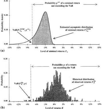
Step 7: Choose the value of the probability pext _{of a minimal return not}

probability is not used.8_{The reason is simple: we do not know of any model}

with a theoretical foundation that allows a link between the VaR and the probability of a return not exceeding the VaR (or more exactly ± VaR, as VaR is usually de®ned to be a positive number). In the extreme value method, in-stead of using the probability related to a basic return, the probability related to a minimal return is used: for example, the probability of a minimal daily return observed over a semester being above a given threshold (the threshold value for a given value of the probability corresponding to the VaR number of the position). As explained in Section 2, for an independent or weakly

de-pendent process, the two probabilities are related by: pext_ˆpn_.9 _{Note that}

when the distribution of returns is exactly known, the extreme value method is equivalent to any classical methods as they give the same VaR number for a

given value ofpor the associated value ofpext_{. To emphasize the dependence of}

the VaR on the distribution and the probability used, the VaR obtained with a

given distribution of returnsFR and a probabilitypis denoted by VaR(FR,p),

and the VaR obtained with the associated exact distribution of minimal returns

FZn and a probability pext is denoted by VaR(FZn; pn). Under the condition

pext_ˆpn_{, we have VaR(F}

Zn;pn)ˆVaR(FR,p).

The choice of the de®nition of the probability is guided by the statistical result concerning the extremes, presented is Section 2. The extreme value theorem shows that the link between the probability related to a minimal re-turn and the VaR can be developed on theoretical grounds. The strength of the method is great as the asymptotic distribution of extremes is compatible with many statistical models used in ®nance to describe the behavior of returns.

The choice of the value of probabilitypext_{is arbitrary (as in other methods).}

However, several considerations can guide this choice: the degree of ®nancial stability required by regulators (for example, the Basle Committee (1996a)

presently imposes a value for probabilityp equal to 0.99 implying a value for

probabilitypext _{equal to 0.99}n _{assuming weak dependence or independence of}

returns), the degree of risk accepted by the shareholders of ®nancial institu-tions, and the communicability of the results in front of the Risk Committee of the banks. For example, the VaR computed with a value of 95% for the

8_{The existing VaR methods of the classical approach use the probability of an unfavorable move}

in market prices under normal market conditions during a day or a given time-period, and then deduce the VaR with a statistical model. For example, the VaR computed by RiskMetricsTM

developed by JP Morgan (1995) corresponds to the probability of observing an unfavorable daily move equal to 5% (equivalent to the probabilitypof a return not exceeding the VaR equal to 95%). In RiskMetricsTM_{, the link between the probability and the VaR is realized with the normal}

distribution.

9_{The equationp}ext_ˆpn _{is still valid in the case of weak dependence. In the case of strong}

probabilitypext_{of a minimal return selected on a semester basis corresponds to}

the expected value of the decennial shock often considered by banks.

Step 8:Compute the VaR of the position.The last step consists of computing the VaR of the position with the asymptotic distribution of minimal returns previously estimated. The full model contains the following parameters: the

frequencyfand the number of basic returnsnfrom which minimal returns are

selected, the three parameters an, bn and sof the asymptotic distribution of

minimal returnsF_Zasymp_n , and the probabilitypext_{of observing a minimal return}

not exceeding the VaR. For processes presenting strong dependence, if the

value of probabilitypext _{is derived from the value of probabilityp using the}

equation pext_{ˆ …p}n_†h_{, then the extremal index h for minimal returns is also}

needed.

Considering the case of a fully aggregated position, the VaR expressed as a percentage of the value of the position is obtained from the estimated as-ymptotic distribution of minimal returns:

pext_ˆ1ÿFasymp Zn …ÿVaR† ˆ exp " ÿ 1 ‡s ÿVaRÿbn an 1=s# …6† leading to VaRˆ ÿb_n‡an s‰1ÿ …ÿln…pext††sŠ: …7†

This ``full'' valuation method used to compute the VaR of a market position requires the construction of the history of returns of the entire position. For complex positions containing many assets or with a time-changing composi-tion, it may be time-consuming to rebuild the history of returns of the position and re-estimate the asymptotic distribution of minimal returns every time the VaR of the position has to be computed. For this reason, it may be more ef-®cient to decompose the position on a limited number of risk factors (such as interest rates, foreign currencies, stock indexes and commodity prices) and compute the VaR of the position in a simpler manner with a risk-aggregation formula. Such a method is presented next.

3.2. The extreme value method for a position decomposed on risk factors

The risk-aggregation formula relates the VaR of the position to the sensi-tivity coecients of the position on risk factors, the VaR of long or short positions in risk factors and the correlation between risk factors. In this way, the computational work is reduced to the estimation of the multivariate dis-tributions of both minimal and maximal returns of risk factors (which is done once for all) and to the calculation of the sensitivity coecients of the position on risk factors (which is repeated every time the composition of the position changes).

A simple ad hoc risk-aggregation formula is used here to compute the VaR

of a position.10_{Consideringqrisk factors, the VaR of a position characterized}

by the decomposition weights…wi†iˆ1;q, is given by

VaRˆ  Xq iˆ1 Xq jˆ1 q_ijwiwjVaRiVaRj v u u t _{; …8†}

where VaRi represents the VaR of a long or short position in risk factori,wi

the sensitivity coecient of the position on risk factoriandqij the correlation

of extreme returns on long or short positions in risk factorsiandj.

For each risk factor, the VaR of a long position, denoted by

VaRl

i…FZasympn ; pext†, is computed with Eq. (7) using the parameters of the

marginal distribution of minimal returns. Similarly, the VaR of a short

posi-tion, denoted by VaRs

i…FYasympn ; pext†, is computed with the same equation using

the parameters of the marginal distribution of maximal returnsF_Yasymp_n .

Considering two risk factors i and j, four types of correlation of extreme

returnsq_ijcan be distinguished according to the type of position (long or short)

in the two risk factors. For a position long (short) in both risk factorsiandj,

the correlationq_ij corresponds to the correlation between the minimal

(maxi-mal) returns of risk factorsiandj. For a position long (short) in factoriand

short (long) in factorj, the correlation q_ij corresponds to the correlation

be-tween the minimal (maximal) return of risk factoriand the maximal (minimal)

return in factorj. To emphasize the dependence on the type of position (long or

short), the four correlation coecients are denoted byqll

ij,qssij,qlsij andqslij.

In the case of total dependence (qijˆ1 for all i and j), the VaR of the

position is equal to the sum of the weighted VaR of each risk factor,_P

q

iˆ1wiVaRi. In the case of independence (qijˆ0 for alli andj, i6ˆj), the VaR of the position is equal to the square root of the weighted sum of the squared VaR of each risk factor, Pq_iˆ1…wiVaRi†2

q

:

To summarize, for a position decomposed on a given set ofq risk factors,

the VaR can be formally written as VaR … †wi iˆ1;q; VaRli…FZasympn ; p

ext_† ÿ iˆ1;q; VaRsi…FYasympn ; p ext_† ÿ iˆ1;q; qab ij a;bˆlors i;jˆ1;q :

10_{This formula is inspired by the formula used in the variance/covariance method. In the case of}

normality, the VaR obtained with the position decomposed on risk factors and based on the risk-aggregation formula (8) with the VaRs of risk factors and correlation coecients classically computed corresponds to the VaR obtained with the fully aggregated position.

The method needs the estimation of 6q parameters of the marginal

distribu-tions of both minimal and maximal returns used to compute the 2qVaRs for

long and short positions in risk factors, and the estimation of 4q correlation

coecients of the multivariate distribution of extreme returns used to aggre-gate the VaRs of risk factors.

The extreme value method takes explicitly into account the correlation be-tween the risk factors during extreme market conditions. It has often been argued that there is a rupture of correlation structure in periods of market stress. For example, using multivariate GARCH processes, Longin and Solnik (1995) conclude that correlation in international equity returns tends to in-crease during volatile periods. Applying multivariate extreme value theory, Longin and Solnik (1997) ®nd that correlation in international equity returns depends on the market trend and on the degree of market volatility. Correla-tion between extreme returns tends to increase with the size of returns in down-markets and to decrease with the size of returns in up-down-markets.

3.3. Positions with derivatives

The VaR of positions with classical options is usually computed by the delta-gamma method to take into account the non-linearity. The VaR of po-sitions with more complex options is often obtained with a Monte Carlo simulation method since no analytical formula is available. With non-linearity, the tail behavior of the distribution is a critical issue. Although the extreme value method may be dicult to implement straightforwardly, extreme value theory may be very useful for determining a model for generating returns from the point of view of extreme events. For example, the non-rejection of the

Frechet distribution would suggest fat-tailed distributions such as a Student

distribution or a GARCH process. The non-rejection of the Gumbel distri-bution for extreme returns would suggest thin-tailed distridistri-butions such as the normal distribution or a discrete mixture of normals. The non-rejection of the Weibull distribution for extreme returns would suggest that bounded

distri-butions with no tails may be used to describe returns. 11_{Parameters from these}

models may be estimated by considering the extremes. For example, the

11_{Note that if a given distribution of returns implies a particular (Frechet, Gumbel or Weibull)}

distribution of extreme returns, the reverse is not true. For example, a Student distribution for returns implies a Frechet distribution for extreme returns, but a Frechet distribution for extreme returns does not necessarily imply a Student distribution for returns. Results about the extremes should be used to infer information about the tails of the distribution only. It should not be used to infer information about the whole distribution as the center of the distribution is not considered by extreme value theory.

number of degrees of freedom of a Student distribution and the degree of persistence in a GARCH process are directly related to the tail index value.

In an extreme value analysis using observed data, it is the historical distri-bution that is studied. However, for evaluating a position with derivatives, one may need a risk-neutral distribution. Using results for the normal distribution

(Leadbetter et al., 1983, pp. 20±21), in a worlda la Black±Scholes, the

risk-neutral asymptotic distribution of extreme returns di€ers from the historical

one by the value of the location parameter only:b

nˆbnÿ …lr0†, where the

asterisk refers to the risk-neutrality, and wherelandr0 _{represent respectively}

the expected return and the risk-free interest rate over a time-period of lengthf.

The scale parameter and the tail index are una€ected by the change of

distri-bution:a

nˆan andsˆsˆ0. For other processes (such as a mixed di€usion

process with jumps or a GARCH process), all three parameters may be a€ected by the change of probability.

3.4. Conditional VaR based on extreme values

Extreme value theory gives a general result about the distribution of ex-tremes: the form of the limiting distribution of extreme returns is implied by many di€erent models of returns used in ®nance (the normal distribution, a discrete mixture of normals, the Student distribution, the stable Paretian distribution, ARCH processes...). Such generality may also mean a lack of re®nement. For example, as the asymptotic extreme value distribution is largely unconditional, the VaR given by the extreme value method is inde-pendent of the current market conditions. In practice, everyday risk man-agement may be improved by taking into account the current market conditions. Thus it may be useful to investigate conditional VaR based on extreme values.

3.5. Related works

Boudoukh et al. (1995) also consider the distribution of extreme returns. They do not use the asymptotic results given by extreme value theory but derive exact results by assuming a normal distribution for returns. In a non-parametric setting Dimson and Marsh (1997) consider the worst realizations of the portfolio value to compute the risk of a position. Danielsson and De Vries (1997) and Embrechts et al. (1998) use a semi-parametric method to

compute the VaR. In both works, the tail index is estimated with HillÕs

esti-mator, which can be used for the Frechet type only. Note that the Weibull

distribution is sometimes obtained, and the Gumbel distribution is often not rejected by the data (some foreign exchange rates and non-US equity returns for example).

4. Examples of application

The case of a fully aggregated position is illustrated with long and short positions in the US equity market. To illustrate the case of a position de-composed on risk factors, long, short and mixed positions in the US and French equity markets are considered.

Table 1

Estimation of the parameters of the asymptotic distributions of extreme daily returns on the S&P 500 Index observed over time-periods of increasing length: 1 week, 1 month, 1 quarter and 1 se-mestera

Length of the selection

period Scaleparameteran

Location parameterbn

Tail index

s Goodness-of-®ttest statistics (A)Minimal daily returns

1 week…Tˆ5† 0.492 )0.518 )0.183 2.770 …fˆ1;nˆ5;Nˆ1;585† (0.009) (0.013) (0.020) [0.001] 1 month (Tˆ21) 0.533 )1.074 )0.148 1.371 …fˆ1;nˆ21;Nˆ377† (0.023) (0.030) (0.031) [0.085] 1 quarter…Tˆ63† 0.585 )1.451 )0.302 )1.040 …fˆ1;nˆ63;Nˆ125† (0.049) (0.059) (0.070) [0.851] 1 semester…Tˆ125† 0.623 )1.726 )0.465 )0.229 …fˆ1;nˆ125;Nˆ63† (0.085) (0.091) (0.128) [0.591] (B)Maximal daily returns

1 week…Tˆ5† 0.501 0.572 )0.084 3.291 …fˆ1;nˆ5;Nˆ1;585† (0.012) (0.013) (0.032) [<0.001] 1 month…Tˆ21† 0.544 1.158 )0.140 0.938 …fˆ1;nˆ21;Nˆ377† (0.025) (0.032) (0.042) [0.174] 1 quarter…Tˆ63† 0.705 1.597 )0.104 0.516 …fˆ1;nˆ63;Nˆ125† (0.053) (0.071) (0.066) [0.303] 1 semester…Tˆ125† 0.845 1.985 )0.060 )0.139 …fˆ1;nˆ125;Nˆ63† (0.087) (0.118) (0.082) [0.555]

a_{This table gives the estimates of the three parameters of the asymptotic distribution of extreme}

daily returns selected over time-periods of increasing lengthTas indicated in the ®rst column. Estimation results are given for the distribution of minimal daily returns (Panel A) and for the distribution of maximal daily returns (Panel B). The scale and location parameters (anandbn) and

the tail index (s) are estimated by the maximum likelihood method. Standard errors of parameters' estimates are given below in parentheses. The database consists of daily returns on the S&P 500 index over the period January 1962±December 1993 (7927 observations). Extreme daily (fˆ1) returns are selected over non-overlapping sub-periods of length ranging from 1 week to 1 semester. A minimal (maximal) daily return corresponds to the lowest (highest) daily return on the S&P 500 index over a given sub-period. The number of selected extremes (N) is inversely related to the length of the selection period (T) or equivalently to the number of daily returns from which extreme re-turns are selected (n). The last column indicates the result of Sherman's goodness-of-®t test with the p-value (probability of exceeding the test-value) given below in brackets. The 5% con®dence level at which the null hypothesis of adequacy (of the estimated asymptotic distribution of extreme returns to the empirical distribution of observed extreme returns) can be rejected, is equal to 1.645.

4.1. The case of a fully aggregated position

The extreme value method presented in Section 3.1 is now applied to the computation of the VaR of both long and short positions in the Standard and

PoorÕs 500 index (this widely available data are used here to allow an easy

replication of the results). Estimation results of the asymptotic distribution of extreme returns are ®rst presented. VaRs are then computed for di€erent values of the probability of an extreme return not exceeding the VaR. The sensitivity of VaR results to the frequency and to the length of the selection period, and the impact of the stock market crash of October 1987 on VaR results are also studied. The VaR given by the extreme value method is also compared with the VaR given by classical methods. Finally, capital requirements are computed in order to assess the regulation of market risks.

4.1.1. Estimation of the asymptotic distribution of extreme S&P 500 index returns

Results of the estimation of the parameters of the asymptotic extreme value distribution are given in Table 1 for minimal returns (Panel A) and for

max-imal returns (Panel B). Extreme daily (f ˆ1 day) returns are observed over

time-periods ranging from one week (T ˆ5 days) to one semester (T ˆ125

days). The database consists of daily returns on the S&P 500 index over the period January 1962±December 1993. Looking at a long time-period (without important structural changes) allows consideration of a variety of market conditions that may occur again in the future. Returns are de®ned as loga-rithmic index price changes. Considering the results for minimal daily returns: the scale parameter increases from 0.492 to 0.623, indicating that the negative extremes are more and more dispersed; the location parameter increases (in absolute value) from 0.518 to 1.726, showing that the average size of negative extremes is larger and larger; the tail index value is always negative and is

between)0.148 and)0.465, implying that the limiting distribution is a Frechet

distribution.12 _{In other words, the asymptotic distribution of minimal daily}

returns shifts to the left and spreads while the shape of the distribution, and specially the way the left tail decreases, remains the same. As the extreme value

distribution is a Frechet distribution, Hill's estimator based on tail

observa-tions can be used for the tail index. Following the procedure used in Jansen and De Vries (1991), the tail index estimate for the left tail is equal to)0.290 with a standard error of 0.043.

12_{A Frechet distribution for extreme returns in the US equity market has been found by Jansen}

and De Vries (1991), Loretan and Phillips (1994) and Longin (1996). Considering other international equity markets, Longin and Solnik (1997) ®nd that all types of extreme value distribution (Frechet, Gumbel and Weibull) are obtained.

A likelihood ratio test shows that the Gumbel distribution (and a fortiori the

Weibull distribution) is always rejected in favor of the Frechet distribution.

The test is distributed as a chi-square variable with one degree of freedom

(obtained by di€erence in the number of parameters in the Frechet and Gumbel

distributions). For example, in the case of minimal returns selected over a

semester, the value of the test is equal to 40.545 with ap-value (probability to

exceed the test value) less than 0.001.

Sherman's goodness-of-®t test indicates that the hypothesis of adequacy (of the estimated asymptotic distribution of extreme returns to the empirical dis-tribution of observed returns) is not rejected at the 5% con®dence level when extreme daily returns are selected over time-periods longer than a month. For extremes selected over a week, the test statistic is equal to 2.770 and is higher than the threshold value of 1.645 associated with a 5% con®dence level. For extremes selected over a month, a quarter and a semester, the test statistics are

respectively equal to 1.371, )1.040 and )0.229, and are lower than the

threshold value. The exact distribution of minimal returns can then be safely replaced by the asymptotic distribution as long as minimal returns are selected over time-periods of length greater than a month. Similar comments apply to maximal daily returns. However, the right tail appears less heavy than the left tail, and the Gumbel distribution for maximal returns is not rejected by the data.

The impact of the stock market crash of October 1987 (the greatest

obser-vation associated with a record-low return of)22.90%) on the estimation of

the parameters of the distribution of minimal returns is also investigated. Considering minimal daily returns selected over a semester, the whole sample

contains 63 observations…N ˆ63†. From Table 1A the parameters' estimates

are with the standard error in parentheses: 0.623 (0.085) for the scale

param-eter,)1.726 (0.091) for the location parameter, and)0.465 (0.128) for the tail

index. Removing the observation of the October 1987 crash from the sample

(Nis now equal to 62) and estimating the distribution of minimal returns again,

the parameters' estimates are now: 0.604 (0.054) for the scale parameter,

)1.748 (0.064) for the location parameter and)0.301 (0.093) for the tail index.

The impact of the greatest observation is largest on the tail index, while the two standardizing coecients are changed slightly. By dropping the observation of the stock market crash of October 1987, the estimated distribution appears to be less fat-tailed (the tail index is closer to zero). Although the di€erence is not statistically signi®cant, the economic impact in terms of VaR and regulatory capital requirement may be worth studying.

The Basle Committee (1996a) allows banks to consider price shocks equivalent to a short holding period such as a day, but it recommends a holding period of 10 days. The behavior of the asymptotic distribution under temporal aggregation is not speci®ed by extreme value theory although the tail index value should remain the same, as shown by Feller (1971, p. 279).

For this reason, asymptotic distributions of extreme returns of various fre-quencies are also estimated. Estimation results are given in Table 2 for minimal returns (Panel A) and for maximal returns (Panel B). Three values

are used for frequency f: 1, 5 and 10 days. Empirically, the asymptotic

dis-tribution of minimal (maximal) returns spreads and shifts to the left (right). For example, considering minimal returns, the scale parameter is equal to 0.623 for one-day returns, 1.098 for ®ve-day returns and 1.875 for 10-day

returns, and the location parameter is equal to )1.726 for one-day returns,

)2.746 for ®ve-day returns and )3.244 for 10-day returns. Such a result was

expected as low-frequency returns are more volatile than high-frequency

re-turns. The tail index value is always negative (between )0.465 and )0.134)

Table 2

Estimation of the parameters of the asymptotic distributions of extreme returns on the S&P 500 Index of various frequencies: 1, 5 and 10 daysa

Frequency of returns Scale parameteran

Location parameterbn

Tail index

s Goodness-of-®ttest statistics (A)Minimal returns

One-day returns…f ˆ1† 0.623 )1.726 )0.465 )0.229 …Tˆ125;nˆ125;Nˆ63† (0.085) (0.091) (0.128) [0.591] Five-day returns…fˆ5† 1.098 )2.746 )0.319 )0.599 …Tˆ125;nˆ25;Nˆ63† (0.136) (0.160) (0.120) [0.725] Ten-day returns…fˆ10† 1.875 )3.244 )0.134 0.499 …Tˆ120;nˆ12;Nˆ63† (0.208) (0.272) (0.096) [0.309] (B)Maximal returns One-day returns…f ˆ1† 0.845 1.985 )0.060 )0.139 …Tˆ125;nˆ125;Nˆ63† (0.087) (0.118) (0.082) [0.555] Five-day returns…fˆ5† 1.207 3.033 )0.147 )1.929 …Tˆ125;nˆ25;Nˆ63† (0.138) (0.176) (0.115) [0.973] Ten-day returns…fˆ10† 1.606 3.834 )0.100 )0.243 …Tˆ120;nˆ12;Nˆ63† (0.181) (0.239) (0.115) [0.596]

a_{This table gives the estimates of the three parameters of the asymptotic distribution of extreme}

returns of various frequencies f as indicated in the ®rst column. Estimation results are given for the distribution of minimal returns (Panel A) and for the distribution of maximal returns (Panel B). The scale and location parameters (anandbn) and the tail index (s) are estimated by the maximum

likelihood method. Standard errors of parameters' estimates are given below in parentheses. The time-series of returns of various frequencies are built from the database of daily returns on the S&P 500 index over the period January 1962±December 1993. The parameternis adjusted such that extreme returns of all three frequencies are selected over non-overlapping semesters (Tˆ125 for one-day and ®ve-day returns andT ˆ120 for 10-day returns). The last column indicates the result of Sherman's goodness-of-®t test with thep-value (probability of exceeding the test-value) given below in brackets. The 5% con®dence level at which the null hypothesis of adequacy (of the esti-mated asymptotic distribution of extreme returns to the empirical distribution of observed extreme returns) can be rejected, is equal to 1.645.

implying a Frechet extreme value distribution for all frequencies. It seems to decrease slightly for minimal returns while it remains fairly stable for maxi-mal returns.

The extremal index h, which models the relationship between the

depen-dence structure and the behavior of extremes of the process, is also estimated. Using the blocks method presented in Embrechts et al. (1997, pp. 419±421, Eq.

(8.10)), the estimate of h is equal to 0.72 when looking at minimal one-day

returns selected over a semester, and equal to 0.73 when looking at maximal

one-day returns (a threshold value of 5% is used to de®ne return

excee-dances). Higher values ofhare obtained when a lower frequency for returns is

used: 0.84 for minimal 10-day returns selected over a semester and 0.92 for

maximal 10-day returns. These estimates are close to the valuehˆ1 obtained

for the case of weak dependence or independence.

4.1.2. VaR of long and short positions in the S&P 500 index

The estimations obtained above are now used to compute the VaR of positions in the S&P 500 index. Empirical results are reported in Table 3 for a long position (Panel A) and for a short position (Panel B). Two holding

pe-riods are considered: 1 day and 10 days (f ˆ1 and 10). Extremes returns are

selected over time-periods of two di€erent lengths: 1 quarter and 1 semester.

The value of the probabilitypext _{of an extreme return not exceeding the VaR}

ranges from 50% to 99% (a higher probability value meaning a higher risk aversion or a higher degree of conservatism). It is important to compute the VaR for di€erent probability values as it gives an idea of the pro®le of the

expected loss beyond the VaR.13 _{For example, considering a holding period}

of 1 day and minimal returns selected on a semester basis, the VaR is equal to $1.98 for a long position of $100 and for a probability value of 50%. In other words, there is one chance in two that the position loses more than $1.98 in one trading session over a semester. The concept of mean waiting period (also called return period) is useful for interpreting the results. The mean waiting period is de®ned as the average time that one has to wait to see an observation exceeding a given threshold. The mean waiting period for a minimal return less than or equal to level z, denoted by T(z) is equal to 1=F_Zasymp_n …z† or 1/

(1) pext_{), expressed in units of the selection period of minimal returns. The}

mean waiting period that one has to wait to observe a loss greater than $1.98 is then equal to two semesters (or one year). For a value of 95% for the

13_{See Longin (1997b), Embrechts et al. (1998) and Artzner et al. (1999) for a measure of the}

probability pext _{(equivalent to a mean waiting period of 20 semesters or 10}

years), the VaR increases to $5.72. A higher value for pext _{implies a higher}

VaR number. A con®dence band measuring the uncertainty due to the es-timation procedure of the asymptotic extreme value distribution can be Table 3

VaR of long and short positions in the S&P 500 Index computed using the extreme value methoda

Probability of not

exceeding VaR Holding period: 1 day_{Selection period:} Holding period: 10 days

1 quarter Selection period:1 semester Selection period:1 quarter Selection period:1 semester (A)Long position

50% 2.18 1.98 4.12 3.72 (1 year) [2.05, 2.30] [1.88, 2.07] [3.91, 4.33] [3.50, 3.94] 75% 2.98 2.78 5.80 5.41 (2 years) [2.74, 3.23] [2.59, 2.97] [5.49, 6.11] [5.06, 5.77] 90% 4.21 4.20 7.78 7.72 (5 years) [3.68, 4.75] [3.72, 4.68] [7.26, 8.29] [7.05, 8.40] 95% 5.36 5.72 9.23 9.67 (10 years) [4.42, 6.29] [4.77, 6.66] [8.48, 9.98] [8.57, 10.77] 99% 9.07 11.76 12.63 15.19 (50 years) [5.62, 12.52] [7.27, 16.25] [10.86, 14.41] [11.85, 18.54] (B)Short position 50% 2.38 2.26 4.20 4.24 (1 year) [2.26, 2.58] [2.16, 2.37] [4.03, 4.36] [4.05, 4.44] 75% 3.10 3.04 5.54 5.70 (2 years) [2.91, 3.30] [2.89, 3.20] [5.29, 5.79] [5.41, 6.00] 90% 4.02 3.98 7.17 7.53 (5 years) [3.66, 4.37] [3.72, 4.24] [6.74, 7.61] [7.02, 8.04] 95% 4.73 4.69 8.41 8.95 (10 years) [4.18, 5.28] [4.31, 5.08] [7.76, 9.06] [8.17, 9.73] 99% 6.56 6.42 11.44 12.57 (50 years) [5.10, 8.02] [5.48, 7.37] [9.82, 13.07] [10.53, 14.61]

a_{This table gives the VaR of positions in the S&P 500 index computed using the extreme value}

method for various values of the probabilitypext_{of an extreme return not exceeding the VaR, as}

indicated in the ®rst column. The corresponding waiting periods are given below in parentheses. The VaR of a long position (Panel A) is obtained with the estimated asymptotic distribution of minimal returns, while the VaR of a short position (Panel B) is obtained with the estimated as-ymptotic distribution of maximal returns. The VaR is computed for a position of $100, or equivalently, the VaR is expressed as the percentage of the value of the position. Two holding periods are considered: 1 and 10 days (fˆ1 and 10). Extremes returns are selected over non-overlapping time-periods of two di€erent lengths: 1 quarter and 1 semester. The probabilitypext_of

observing an extreme return not exceeding the VaR depends on the length of the selection period (parameterTornfor a given frequencyf):pext_ˆpext_{n†. The probability used to compute the}

VaR with extreme returns selected on a quarterly basis…nˆ63†is related to the one used to compute the VaR computed with extreme returns selected on a semester basis…nˆ125†by using the equation:pext_{63† ˆp}ext_125†63=125_{. The 50% con®dence band is given below in brackets for}

each estimate of VaR. It is estimated from the quantiles of the estimated asymptotic distribution of extreme returns.

computed.14_{For example, for a long position and a probability value of 95%,}

the 50% con®dence band for the VaR estimate of $5.72 is $4.77, $6.66. In other words there is a 50% chance for the VaR to be located between $4.77 and $6.66. The 90% con®dence band is $3.42, $8.01.

Impact of the frequency: From the results reported in Table 3, the VaR

numbers computed from returns with the lower frequency (f ˆ10 days) are

always higher than the VaR computed from returns with the higher frequency

(f ˆ1 day). They are around 90% higher in most of the cases. In order to

compute the regulatory capital requirement, VaR numbers calculated ac-cording to shorter holding periods than 10 days have to be scaled up to 10 days, by the square root of the time factor. For example, VaR obtained from

daily returns would have to be multiplied by a time factor ofp1020. For a

long position and a probability value of 95%, the scaled VaR obtained with

one-day returns is equal to $18.09 …ˆp105:72†21and is thus much higher

than the VaR computed with 10-day returns ($9.67). Such a di€erence suggests that the scaling factor proposed by the Basle Committee may be too high.

Impact of the length of the selection period: The VaR can be computed from

the distribution of extreme returns selected over time-periods of di€erent length as long as it ®ts well the empirical distribution of observed extremes. Of course,

the value of the probabilitypext_{has to be adjusted as this parameter depends on}

the length of the selection period. For two selection periods containingnandn0

basic returns, a simple adjustment rule may bepext_{n† ˆ ‰p}ext_n0_†Šn=n0

. This rule is consistent with i.i.d. processes and also with processes presenting weak or strong dependence. VaR results previously presented for extreme returns se-lected over a semester are now compared with those obtained for extreme re-turns selected over a di€erent time-period. The probability value of 95% used in the case of extreme returns selected over a semester corresponds to a proba-bility value of 97.44%…ˆ0:9563=125_{†for extreme returns selected over a quarter.}

Using the estimates of the parameters given in Table 1A the corresponding VaR numbers for a long position are $5.36 for a selection period of a quarter. This number is not statistically di€erent from the VaR obtained with a selec-tion period of a semester ($5.72). As similar VaR numbers are obtained, the extreme value method seems to be robust to the choice of the length of the selection period.

Impact of the dependence in the data: The relationship between the

depen-dence in the data and the behavior of extremes is modeled with the extremal

indexh. When the probabilitypext_{of an extreme return not exceeding the VaR}

14_{The formula for the estimation error on the quantile estimation is given in Kendall (1994, pp.}

358±359). The estimation risk for VaR is discussed in Jorion (1996). Techniques for verifying the accuracy of VaR can also be found in the recommendations of the Basle Committee on backtesting (1996b) and in Kupiec (1995).

is derived from the probabilityp of a basic return not exceeding the VaR, the

equation pext_{ˆ …p}n_†h _{should be used in the case of strong dependence. Note}

that, as the extremal index is always lower than one, the VaR is always higher in the case of strong dependence than in the case of weak dependence or

in-dependence. Empirically, using the estimate ofh equal to 0.72 obtained with

minimal daily returns selected over a semester, the equation pext_ˆpn_ˆ0:95

becomes pext_{ˆ …p}n_†h_ˆ0:950:72 _{ˆ0:9637 by taking into account the}

depen-dence. The corresponding VaR is equal to $6.60, compared to $5.72 obtained by assuming weak dependence or independence of returns. The impact of de-pendence seems to be less pronounced when a lower frequency for returns is

employed. Using the estimate ofhequal to 0.84 obtained with minimal 10-day

returns selected over a semester, the probabilitypext _{corrected for the e€ect of}

dependence is equal to 95.78%…ˆ0:950:84_{†and the corresponding VaR is equal}

to $10.58 compared to $9.67 obtained by assuming weak dependence or in-dependence of returns. The di€erence in VaR results is not statistically sig-ni®cant but it may be judged quite large from an economic point of view (additional capital is always costly for ®nancial institutions).

Impact of the stock market crash of October 1987: The impact of the stock

market crash of October 1987 on VaR results is also investigated. Using the asymptotic distribution of minimal daily returns selected over a semester, the VaR of a long position is equal to $4.65 by excluding the crash from the set of minimal returns for the estimation, compared with $5.72 by including the crash. From a statistical point of view, the di€erence can be attributed to the tail index, whose value is larger when the return observation of the crash is included in the estimation.

4.1.3. Comparison with classical methods

The VaR given by the extreme value method, VaR(F_Zasymp_n ;pext_{) for a long}

position or VaR(F_Yasymp_n ;pext_{) for a short position, is now compared with the}

VaR given by classical methods, denoted by VaR(FR,p), where FR is a

par-ticular distribution of returns.15 _{To make VaR results given by both}

ap-proaches directly comparable, it is assumed that the probabilitiespext_andpare

related by the equation:pext_ˆpn_{, which is valid under the assumption of weak}

dependence and independence of returns. Four classical VaR methods are considered:

· VaR(Fhis

R ,p) based on the historical distribution of returns, denoted byFRhis.

· VaR(Fnor

R ;p) based on the normal distribution of returns, denoted byFRnor.16

15_{Former empirical studies on VaR include Beder (1995) and Jackson et al. (1997).}

16_{Over the period January 1962±December 1993, the estimates of the meanland standard}

deviationrof the normal distribution of returns are 0.027% and 0.883% for one-day returns, and 0.264% and 2.852% for 10-day returns.

· VaR(FGARCH

Rt ;p) based on the conditional GARCH process. A

GARCH(1, 1) is used here. Return Rt observed at time tis assumed to be

drawn from a conditional normal distribution denoted byFGARCH

Rt . The

con-ditional variance rt2 of this distribution is given by r2t ˆa0‡a1e2tÿ1

‡b1r2tÿ1, where parameter a1 represents the persistence in volatility of the

latest squared innovation et2_ÿ1, and parameter b1 measures the persistence

in volatility of the past variancert2ÿ1.17

· VaR(FEWMA

Rt ;p) based on the exponentially weighted moving average

(EWMA) process for the variance used in RiskMetricsTM_{. Return Rt}

ob-served at timetis assumed to be drawn from a conditional normal

distribu-tion denoted byFEWMA

Rt . The conditional variancert2of this distribution is

given by r2

t ˆ …1ÿk†e2tÿ1‡kr2tÿ1, where the parameterk, called the decay

factor, re¯ects the persistence of volatility over time. 18_{This process is an}

in-tegrated GARCH(1, 1) process with the constrainta1‡b1ˆ1.

The methods using the asymptotic extreme value distribution, the empirical distribution and the normal distribution are unconditional as they give the same results whatever the market conditions at the time of estimation. Con-ditional models such as the GARCH and EWMA processes account for the time-varying conditions of the market as they use a normal distribution with time-varying mean and variance. As a consequence, they lead to a VaR which re¯ects the degree of market volatility at the time of estimation.

Empirical VaR results for positions in the S&P 500 index are given in Table 4 for the various methods presented above. The VaR is computed for a long position (Panel A) and a short position (Panel B). Two holding periods are

considered: 1 and 10 days (f ˆ1 and 10). Three values for the probabilitypext

of an extreme return not exceeding the VaR are taken: 50%, 95% and 99% corresponding to waiting periods respectively equal to 1, 10 and 50 years.

Considering a long position and a holding period of 1 day, the VaR based on the historical distribution of returns observed over the period January

1962±December 1993 is equal to $2.06 for a value of 50% for probabilitypext

and to $6.32 for a probability value of 95%. These numbers are close to those obtained with the extreme value distribution: $1.98 and $5.72. Such results are consistent with the good ®t of the extreme value distribution to the data as previously discussed. Note that for very high probability values (99% for ex-ample), the VaR cannot be computed from the historical method because of

17_{The estimates of the three parameters a}

0, a1 and b1 of the GARCH(1, 1) process are

respectively equal to 0.004, 0.094 and 0.904 for one-day returns, and 0.488, 0.141 and 0.807 for 10-day returns.

18_{The estimate of the parameterkof the EWMA process is equal to 0.93 for one-day returns and}

the lack of data. Such a drawback does not exist for the extreme value method

which, as a parametric method, allowsout-of-sampleVaR computations.

The VaR based on the unconditional normal distribution of returns is equal

to $2.22 for a value of the probabilitypext _{equal to 50%. By comparison, the}

VaR based on the asymptotic extreme value distribution is equal to $1.98. For low probability levels, the two methods then lead to similar results. As the normal distribution has thin tails, the VaR computed for more conservative probability levels is not much higher: for example, for a value of probability

pext_{equal to 95%, it is equal to $2.93, a number much lower than that given by}

the extreme value distribution ($5.72). Such a result illustrates the problem of Table 4

VaR of long and short positions in the S&P 500 Index computed using the extreme value method and classical methodsa

Methods used to

compute VaR Holding period: 1 day_{Probability of not exceeding VaR} Holding period: 10 days_{Probability of not exceeding VaR}

50% 95% 99% 50% 95% 99%

(A)Long position VaR(Fasymp Zn ;pext† 1.98 5.72 11.76 3.72 9.67 15.19 VaR(Fhis R ;p) 2.06 6.32 n.c. 3.73 9.58 n.c. VaR(Fnor R ;p) 2.22 2.93 3.31 4.27 7.24 8.70 VaR(FGARCH Rt ;p) 1.01 1.34 1.52 2.12 3.73 4.53 VaR(FEWMA Rt ;p) 0.93 1.24 1.40 1.95 3.41 4.12 (B)Short position VaR(Fasymp Yn ;Pext) 2.26 4.69 6.42 4.24 8.95 12.57 VaR(Fhis R ;p) 2.41 4.65 n.c. 4.01 9.19 n.c. VaR(Fnor R ;p) 2.27 2.98 3.36 4.80 7.77 9.23 VaR(FGARCH Rt ;p) 1.09 1.43 1.60 2.81 4.43 5.22 VaR(FEWMA Rt ;p) 0.99 1.29 1.45 2.48 3.93 4.25

a_{This table gives the VaR of positions in the S&P 500 index computed using various methods as}

indicated in the ®rst column. The VaR is computed for a long position (Panel A) and for a short position (Panel B). Five statistical models are considered: the asymptotic distribution of extreme returns, the historical distribution of returns, the unconditional normal distribution of returns, and GARCH and EWMA processes of returns. The VaR is computed for a position of $100, or equivalently, the VaR is expressed as the percentage of the value of the position. Two holding periods are considered: 1 and 10 days (fˆ1 and 10). Extreme returns are selected over non-overlapping semesters (nˆ125 andTˆ125 for one-day returns andnˆ12 andTˆ120 for 10-day returns). Three values for the probabilitypext_{of an extreme return not exceeding the VaR are}

taken: 50%, 95% and 99% corresponding to waiting periods respectively equal to 1 year, 10 years and 50 years. For the classical VaR methods, the probabilitypof a return not exceeding the VaR is related to probabilitypext_{by the relationp}ext_ˆpn_{, which is valid under the assumption of weak}

dependence or independence of returns. For the conditional models (GARCH and EWMA pro-cesses), the VaR is computed on December 31, 1993 (the last day of the database). For high values of probabilitypext_{(orp), the VaR is not calculable (n.c.) with the historical distribution because of}