On the Capacity of Ad Hoc Wireless Networks
Under General Node Mobility
Michele Garetto, Paolo Giaccone, Emilio Leonardi
Technical report
Abstract— We revisit the problem of characterizing the
ca-pacity of an ad hoc wireless network with n mobile nodes. Grossglauser and Tse (2001) showed that, by exploiting user mobility, it is possible to maintain a constant per-node throughput as the number of nodes grows. Their scheme allows to overcome the throughput decay (at least as 1=
p
n) that affects networks with static nodes, which was first pointed out by Gupta and Kumar (2000). Subsequent works have analyzed the delay-capacity trade-off that arises in mobile networks under various mobility models. Almost invariably, however, available asymptotic results strongly rely on the assumption that nodes are identical, and move according to some ergodic process that is equally likely to visit any portion of the network area. In this paper, we relax such ‘homogeneous mixing’ assumption on the node mobility process, and analyze the network capacity in the more realistic case in which nodes are heterogeneous, and the motion of a node does not necessarily cover uniformly the entire space. We propose a general framework to characterize the capacity of networks with arbitrary mobility patterns, considering both the case of finite number of nodes (also with the support of experimental traces), as well as asymptotic results when the number of nodes grows to infinity.
I. INTRODUCTION AND PREVIOUS WORK
In recent years a significant effort has been devoted by the research community to study the asymptotic performance of ad hoc wireless networks when the number of users increases. Gupta and Kumar [1] consider a model in which n static
nodes randomly placed in a disk of unit area, establish n
source-destination (S-D) communications. They obtain the disheartening result that the throughput available to each S-D pair decreases at least as 1=
p
n, even allowing optimal
scheduling and node placement. Grossglauser and Tse [2] consider a similar scenario in which the nodes are mobile, and show that, in contrast to the fixed node case, the throughput per S-D pair can be kept constant while increasing n. This
nice property was established under the assumption that the trajectories of the nodes are independent, and results for each node into a uniform stationary distribution over the disk of unit area. This mobility pattern is actually a generous one, since it allows each node to equally come in contact with any other node in the network.
Indeed, in real environments, the contact times between the nodes can be highly diverse, as recently pointed out in [3]. Actually, an individual node usually spends most of the time just on a small portion of the entire network area, and rarely goes outside its region of habit. Motivated by
M. Garetto is with Dipartimento di Informatica, Universit`a di Torino, Italy; P. Giaccone and E. Leonardi are with Dipartimento di Elettronica, Politecnico di Torino, Italy. This work was supported by the Italian Ministry of University and Research through CARTOON PRIN-project.
this observation, in [4] the authors considered a restricted mobility model, where each node independently moves along a randomly chosen great circle on the sphere of unit surface. Quite surprisingly, even under this one-dimensional mobility pattern a constant throughput per S-D pair can be sustained.
Since then, the attention of researchers has been mostly attracted by capacity-delay trade-offs [5], [6], [7], [8]. Various mobility models have been considered, such as the simple re-shuffling model [5], Brownian motion [6], different variants of random walks and random way-point [7], [8]. Almost invari-ably, in all these studies nodes are assumed to be identical and independently moving, while their trajectories ‘fill the space over time’. One exception is [9], where the authors study throughput-delay scaling laws for the same one-dimensional mobility pattern considered in [4]. Another study of capacity-delay trade-off under restricted mobility appears in [10]: here the network of unit area is partitioned into square cells, and nodes are restricted to move within one randomly chosen cell; the authors consider two cases in which the cell area either scales as(logn)=nor remains constant, obtaining results close
to Gupta-Kumar and Grossglauser-Tse, respectively.
Apart from the above examples of restricted mobility over great circles or cells, the general question about how anisotropic mobility patterns affect the network capacity has been left behind unanswered. The goal of this paper is to fill the existing gap in the analysis of the throughput capacity of ad hoc wireless networks. We address the general case of heterogeneous nodes with arbitrary mobility patterns. Clearly, there exists an extraordinary huge space of different mobility patterns in between the extreme cases of static nodes (Gupta-Kumar) and complete homogeneous mixing (Grossglauser-Tse). Therefore it is quite interesting to investigate how the network capacity can vary across such a huge space. In this work we are not concerned with delay, but only on throughput. Thus practical implications of our work mainly fit in the context of delay tolerant networks [11].
We remark that we are not the first to consider the capacity of ad hoc wireless networks with heterogeneous nodes. In the particular case of static nodes, several works have already appeared that generalize the results of Gupta-Kumar. The nice deterministic approach proposed in [12] allows to analyze in a simple way non-uniform spatial distribution such as straight lines, or highly dense neighborhoods. The work in [13] inves-tigates the network capacity resulting from asymmetric traffic patterns. In [14] the authors analyze arbitrary node placement and interference constraints using spectral techniques. Several papers have also considered the case of hybrid networks, where an overlay of wired base stations is added to the
ad hoc network [15], [16], [17], [18], with the potential of dramatically improving the available per-node throughput.
To the best of our knowledge, we are the first to consider the general case of heterogeneous mobile nodes. More specifi-cally, we provide the following contributions: i) we formulate the general case as a joint scheduling and routing problem, defining an abstract framework within which the performance analysis of mobile ad hoc networks can be carried out; ii) we precisely characterize the capacity region of a network with finite number of nodes, pointing out several structural properties of the system; iii) we apply the framework to the analysis of a real network, using publicly available traces; iv) we extend the analysis to the asymptotic regime, first estab-lishing some results of general validity, and then considering a few significant examples of anisotropic distributions of the nodes over the area.
II. NETWORKS WITH FINITE NUMBER OF NODES
A. System assumptions and notation
We consider a mobile ad hoc network composed of n
nodes moving according to a general mobility model in-side a bidimensional, compact and convex region A of
area jAj. Let X i
(t) denote the position of node i at
time t and X(t)=(X 1 (t);X 2 (t):::X n (t)) the vector of
nodes’ positions; we define with d ij
(t) the euclidean
dis-tance between mobile i and mobile j at time t, i.e., d ij (t)=jjX i (t) X j (t)jj 2.
We assume the node mobility process to be stationary and ergodic; i.e., given any m-uple (B
1 ;B 2 ;B 3 :::B m ) of
Lebesgue measurable subsets ofA, it results: lim t!1 1 t Z t 0 I (\ i X i ()2B i ) d =E[I (\ i X i (t)2B i ) ℄ w.p.1
whereIrepresents the logical indicator function.
Node s generates traffic for destination d according to a
stationary and ergodic process with average traffic rate sd
bit/s1. We denote with
= [
sd
℄ the corresponding nn
traffic matrix.
We assume that interference between simultaneous trans-missions is described by the well known protocol interference model [1]. However, most of the results obtained in this paper can be extended to the physical interference model [1] too2. According to the protocol interference model, transmission from nodeito nodej at timet at rateris successful only if,
for any other simultaneously transmitting nodek, it holds: d
k j
(t)>(1+)d ij
(t)
for some guard factor>0. Note that according to this
inter-ference model: (i) no node can be either origin or destination of multiple simultaneous transmissions, (ii) a node cannot be simultaneously origin and destination of transmissions.
We denote with Q the set of all possible
transmission-receiver pairs (i;j) (by construction it must be i 6= j). 1Defined with^
(t;)the amount of data generated by a source within the
interval[t;), the traffic is said stationary and ergodic with average rate
iff:E[ ^
(t;t+1)℄=for anyt>0andlim t!1
^
(0;t)=t=w.p.1. 2Note that the protocol interference model has been proved to be
equiv-alent to the physical interference model when each user employs the same power [1].
Subsets of Q in which nodes appear at most once (either
as transmitter or receiver), represent possible transmission configurations, i.e., sets of transmission-receiver pairs (i;j),
which may be simultaneously enabled to communicate at time
t. We denote with the set of all the possible
transmis-sion configurations and with A(t) the set of all
non-interfering (hence, implementable) transmission configurations at time t. The protocol interference model (more in general,
any interference model) induces a correspondence between the vector of instantaneous nodes positions X(t) and the
set of non-interfering transmission configurations A(t); we
formalize this concept introducing functionI mapping vectors
of nodes positions into sets of non-interfering transmission configurations:I(X(t))=A(t).
Given any set Aof implementable transmission
configura-tions, we denote with I 1
(A) the set of node positions X
to which A corresponds through mapping I, i.e.,I 1
(A)= fX:I(X)=Ag.
3 For any
A, we can univocally determine
the probability that A(t) = A, i.e. the probability that
configurations in Aare the only implementable at time t: P(A)=E[I X(t)2I 1 (A) ℄= lim t!1 1 t Z t 0 I X()2I 1 (A) d w.p.1
Note that the above probability depends only on the joint stationary distribution of the node mobility process.
At last, we denote with fT n
g the sequence of random
instants at which the set of implementable transmission con-figurations changes; i.e.,lim
t"T n A(t)6=A(T n ). B. Scheduling policy
The scheduling policy S dynamically selects an
im-plementable transmission configuration S
(t) belonging to A(t)=I(X(t)). In this paper we restrict our investigation to
stationary and ergodic scheduling policies: i.e. those policies for which: E[I (i;j)2 S (t) ℄= lim t!1 1 t Z t 0 I (i;j)2 S () d w.p.1
In general the selection of S
(t)may be influenced by several
dynamical parameters, including instantaneous queues lengths, age of stored information at nodes, etc. Particularly relevant are those scheduling policies driven only byX(t). In this paper
we call stateless and memoryless such scheduling policies. We also introduce the class of simple scheduling policies
^
S, which is a strict subclass of the stateless and memoryless
scheduling policies characterized as follows. At each transition time T
n a transmission configuration
2 A(T n
) is selected
according to a stationary and memoryless (possibly random) rule; the selected transmission configuration is then kept constant in the whole interval [T
n ;T
n+1
). Simple scheduling
policies are fully specified by the conditional probabilities
p ^ S
(;A) that the transmission configurations 2 A are
selected at time T n, given that X(T n )2I 1 (A): p ^ S (;A)=Prf ^ S (T n )=jX(T n )2I 1 (A)g 8Aand 2A 3It can be verified that, for any
A2,I 1
(A)is a convex set ofR 2n
According to scheduling policy S, a communication link is
established between nodes i and j whose average capacity
expressed in bit/s is:
S ij =rE[I (i;j)2 S (t) ℄= lim t!1 r t Z t 0 I (i;j)2 S () d w.p.1
which, in case of simple scheduling policies, can be rewritten as: ^ S ij =r P A2 P 2A I (i;j)2 p ^ S (;A)P(A).
An important question we would like to answer is: “how can we characterize the capacity of the mobile ad hoc network under a scheduling policyS (or
^
S)?” To this end we need to
spend few words on the routing strategy employed to transfer data through the network. The more general and abstract way to define a routing strategy is to specify quantitiesf
sd ij
2[0;1℄
denoting the average fraction of traffic from node s to node d, which is routed through link(i;j), i.e.j followsias relay
node [19]; f sd ii
= 0 by construction. The above quantities f
sd ij
must satisfy the following well known flow conservation constraints: X i f sd ij X k f sd jk = 8 < : 1 forj=d 0 forj6=dandj 6=s 1 forj=s (1)
A routing strategy specified by a set of f sd ij
satisfying (1) can be easily implemented by the following simple hop-by-hop routing algorithm R: every nodei in the network, upon
reception of new data from sources, destined tod, routes them
by selecting nodej as next hop with probabilityf sd ij = P k f sd ik .
C. Traffic sustainability and capacity region
In this subsection we analyze the performance of a mobile ad hoc network comprising n users, obtaining a precise
characterization of its capacity region. We emphasize that our results are fairly general since only stationarity and ergodicity of traffic and mobility processes are required. We remark that, in our framework, the nodes movements are not constrained to be independent of each other.
Definition 1: We denote with Z(t) the network backlog,
that is, the amount of traffic (in bits) already generated by sources that has not yet been delivered to destinations at time
t.
Definition 2: Traffic is sustainable if there exists a
scheduling policy S and a routing strategy R, such that: limsup
t!1
Z(t)=t=0w.p.1.
Definition 3: Traffic is strongly sustainable if there
exists a simple scheduling policy ^
S and a routing strategyR,
such that:limsup t!1
Z(t)=t=0w.p.1.
We are now in a position to state our first result:
Theorem 1: A mobile ad hoc network sustains a traffic,
if a scheduling policySand a routing strategyRcan be found
such that: X sd sd f sd ij S ij 8i;j (2)
Moreover, if a simple scheduling policy ^
S and a routing
strategyRcan be found such that: X sd sd f sd ij ^ S ij 8i;j (3)
the mobile ad hoc network strongly sustains traffic .
Proof: The dynamics of the system can be described by a network of queues representing the evolution of the backlog at different nodes. We suppose that every nodei is equipped
with n 1 separate transmission queues, each one storing
data to be routed through a different nodej. Upon reception,
new data are immediately routed according to policy Rand
enqueued in the transmission queue associated to the next hop. Transmission queues are served at fixed rateraccording
to a FCFS service policy, during the periods of activity of the corresponding link (i;j). Note that, by construction, the
average service rate in bit/s of the transmission queue of link
(i;j)is S ij
. The network of queues describing the system falls in the class of generalized Kelly networks, which are stable under the condition that no queues are overloaded [20]. Being, by construction, the load at the queue of link (i;j) equal to P sd sd f sd ij = S ij
1, the assert follows immediately 4.
As a corollary, we get a strict characterization of the traffic matrices which are strongly sustainable:
Proposition 1: A traffic matrix =[ sd
℄is strongly
sus-tainable iff a set off sd ij
2[0;1℄,8i;j;s;dandp(;A)2[0;1℄ 8A;2Acan be found satisfying the following equations:
8 > > > > < > > > > : f sd ij satisfies (1) 8i;j;s;d X 2A p(;A)=1 8A2 X sd sd f sd ij r X A2 X 2A I (i;j)2
p(;A)P(A) 8i;j
Definition 4: The capacity region of the mobile ad hoc
network is the set of all sustainable traffic matrices.
Definition 5: The restricted capacity region of the mobile
ad hoc network is the set of all strongly sustainable traffic matrices.
Note that the restricted capacity region, by construction, depends on nodes mobility only via the joint stationary distri-bution of nodes. We can now state the following fundamental result:
Theorem 2: If traffic matrixis sustainable, then it is also
strongly sustainable.
Proof: Let S be the stationary and ergodic scheduling
policy which sustains . Define for every configuration A
and every2A: q S (;A)=Prf S (t)=jX(t)2I 1 (A)g= lim t!1 1 t Z t 0 I S ()=jX()2I 1 (A) d w.p.1
Due to the ergodicity of the mobility process and of the scheduling policy, the above quantities are well defined. It is immediate to verify that:
P 2A
q S
(;A) = 1. Thus
considering a stationary, simple scheduling policy ^
S such that p ^ S (;A) =q S (;A), it follows, by construction: S ij = ^ S ij 8i;j.
The previous result has three significant implications: i) the class of simple policies achieves maximum throughput, i.e., no gain in terms of throughput can be obtained by adopting complex scheduling policies that select transmission configura-tions by considering dynamical variables such as instantaneous
4WhenP sd f sd = S
queues lengths, age of stored information at the nodes, etc; ii) a tight characterization of the capacity region is provided by Proposition 1; iii) the capacity region depends on the mobility process only through the joint-stationary distribution of nodes. This result extends and generalizes recent findings in [8]. At last,
Corollary 1: The capacity region of an ad hoc wireless
network with mobile nodes is convex.
Proof: Let
1 and
2 be two sustainable traffic
ma-trices. Let ^ S
1 and ^ S
2 be two simple scheduling policies
which sustain 1 and
2 respectively. Any traffic pattern
=
1
+(1 )
2, with
0 1, is sustainable
by the simple policy ^
S defined according to: p ^ S (;A) = p ^ S1 (;A)+(1 )p ^ S2
(;A), 8A; 2A. Note that ^ S, at
time t, with probability emulates ^ S
1 and with probability (1 )emulates
^ S
2.
D. Contact graph: throughput and routing
To understand the relationship between the scheduling pol-icy and the routing strategy, we first need to characterize which traffic patterns are sustainable by employing an assigned scheduling policyS. Observe that the capacities
5
ij
associ-ated to the communication links are univocally determined, once the scheduling policyShas been selected. Thus a
(capac-itated) graphG(V;E) whose vertices correspond to network
nodes and capacitated edges correspond to communication links, fully characterizes the mobile ad hoc network adopting
S. In the following we refer toG(V;E)with the term contact
graph. Therefore, the routing problem through the mobile ad hoc network adoptingScan be formalized in terms of a
multi-commodity flow problem on the contact graph.
Proposition 2: A traffic matrix=[ sd
℄can be sustained
employing a policy S iff the multi-commodity flow problem
defined by (1) and (2), where communication link capacities are determined byS, admits a feasible solution. In such a case
the set of variablesf sd ij
univocally defines the routing strategy
R.
An alternative, partial characterization of the sustainable re-gion achievable by scheduling policy S (i.e. the set of = [
sd
℄ that can be sustained employing S) can be provided in
terms of the capacities associated to cuts of the contact graph.
Proposition 3: Traffic =[ sd
℄ is sustainable by policy S only if, for any partition(D;
D)of the nodes, it results: X s2 D X d2D sd X s2 D X d2D sd (4)
For undirected Graphs G(V;E), it was proven in [21] that
traffic is guaranteed to be sustainable if the ratio between
the minimum value of the r.h.s. and the maximum value of the l.h.s. is!(logm)beingm the number of flows.
6
Consider a network adopting a scheduling policyS and a
routing strategyR, under a sustainable traffic pattern. Let 5To simplify the notation we omit, in this section, the explicit dependency
from the scheduling policyS. 6Given two functions
f(n) 0 and g(n) 0: f(n) = o(g(n)) means lim
n!1
f(n) =g(n) = 0; f(n) = O(g(n)) means limsup
n!1
f(n) =g(n) = < 1; f(n) = !(g(n)) is equivalent to g(n) = o(f(n)); f(n) = (g(n)) is equivalent to g(n) = O(f(n));
finally,f(n)=(g(n))meansf(n)=O(g(n))andg(n)=O(f(n)).
0.001 0.01 0.1 1 10 100 1000 10000 100000 1e+06 P[X>x] Capacity [sec]
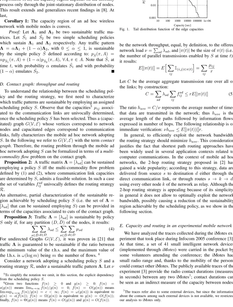
Fig. 1. Tail distribution function of the edge capacities
be the network throughput, equal, by definition, to the offered network load =
P sd
sd, and
j(t)jbe the size of(t)(i.e.,
the number of parallel transmissions enabled byS at timet);
it results: E[j(t)j℄=E h X ij I (i;j)2(t) i = X ij ij r
Let C be the average aggregate transmission rate over all of
the links; by construction:
C= X sd sd X ij f sd ij rE[j(t)j℄ (5) The ratioh ave
=C=represents the average number of times
that data are transmitted in the network; thus h
ave is the
average length of the paths followed by information flows, expressed in number of hops. The following relationship is of immediate verification:h
ave
E[j(t))j℄r.
In general, to efficiently exploit the network bandwidth, the routing strategy should minimizeh
ave. This consideration
justifies the fact that shortest path routing approaches have been widely used in several application contexts related to computer communications. In the context of mobile ad hoc networks, the 2-hop routing strategy proposed in [2] has gained a wide popularity; according to this strategy, data are delivered from source s to destination d either through the
direct communication link, or through routes s ! k ! d,
using every other nodekof the network as relay. Although the
2-hop routing strategy is appealing because of its simplicity, in general it does not allow to optimally exploit the network bandwidth, possibly causing a reduction of the sustainability region achievable by the scheduling policy, as we show in the following section.
E. Capacity and routing in an experimental mobile network We have analyzed the traces collected during the iMotes ex-periment that took place during Infocom 2005 conference [3]. At that time, a set of 41 small intelligent network devices (implemented through iMotes) were carried in the pocket by some volunteers attending the conference; the iMotes had small radio range and, thanks to the mobility of the person, could contact other iMotes. The publicly available traces of the experiment [3] provide the radio contact durations (measured in seconds) between any two iMotes7; contact durations can
be seen as an indirect measure of the capacity between nodes.
7The traces refer also to some external devices, but since the information
about the contacts among such external devices is not available, we restricted our analysis to iMotes only.
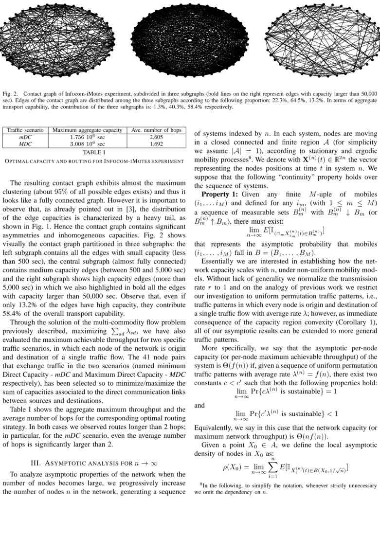
Capacity <500 sec Capacity 500-5000 sec Capacity >5000 sec
Fig. 2. Contact graph of Infocom-iMotes experiment, subdivided in three subgraphs (bold lines on the right represent edges with capacity larger than 50,000 sec). Edges of the contact graph are distributed among the three subgraphs according to the following proportion: 22.3%, 64.5%, 13.2%. In terms of aggregate transport capability, the contribution of the three subgraphs is: 1.3%, 40.3%, 58.4% respectively.
Traffic scenario Maximum aggregate capacity Ave. number of hops
mDC 1:75610 6 sec 2.605 MDC 3:00810 6 sec 1.692 TABLE I
OPTIMAL CAPACITY AND ROUTING FORINFOCOM-IMOTES EXPERIMENT The resulting contact graph exhibits almost the maximum clustering (about95%of all possible edges exists) and thus it
looks like a fully connected graph. However it is important to observe that, as already pointed out in [3], the distribution of the edge capacities is characterized by a heavy tail, as shown in Fig. 1. Hence the contact graph contains significant asymmetries and inhomogeneous capacities. Fig. 2 shows visually the contact graph partitioned in three subgraphs: the left subgraph contains all the edges with small capacity (less than 500 sec), the central subgraph (almost fully connected) contains medium capacity edges (between 500 and 5,000 sec) and the right subgraph shows high capacity edges (more than 5,000 sec) in which we also highlighted in bold all the edges with capacity larger than 50,000 sec. Observe that, even if only 13.2% of the edges have high capacity, they contribute 58.4% of the overall transport capability.
Through the solution of the multi-commodity flow problem previously described, maximizing
P sd
sd, we have also
evaluated the maximum achievable throughput for two specific traffic scenarios, in which each node of the network is origin and destination of a single traffic flow. The 41 node pairs that exchange traffic in the two scenarios (named minimum Direct Capacity - mDC and Maximum Direct Capacity - MDC respectively), has been selected so to minimize/maximize the sum of capacities associated to the direct communication links between sources and destinations.
Table I shows the aggregate maximum throughput and the average number of hops for the corresponding optimal routing strategy. In both cases we observed routes longer than 2 hops; in particular, for the mDC scenario, even the average number of hops is significantly larger than 2.
III. ASYMPTOTIC ANALYSIS FORn!1
To analyze asymptotic properties of the network when the number of nodes becomes large, we progressively increase the number of nodesnin the network, generating a sequence
of systems indexed by n. In each system, nodes are moving
in a closed connected and finite region A (for simplicity
we assume jAj = 1), according to stationary and ergodic
mobility processes8. We denote withX (n)
(t)2R 2 n
the vector representing the nodes positions at time t in system n. We
suppose that the following “continuity” property holds over the sequence of systems.
Property 1: Given any finite M-uple of mobiles (i
1 ;:::i
M
) and defined for any i
m, (with
1 m M)
a sequence of measurable sets B (n) m with B (n) m # B m (or B (n) m "B
m), there must exist: lim n!1 E[I (\mX (n) im (t)2B (n) m ) ℄
that represents the asymptotic probability that mobiles
(i 1 ;:::;i M )fall inB=(B 1 ;:::;B M ).
Essentially we are interested in establishing how the net-work capacity scales withn, under non-uniform mobility
mod-els. Without lack of generality we normalize the transmission rate r to 1 and on the analogy of previous work we restrict
our investigation to uniform permutation traffic patterns, i.e., traffic patterns in which every node is origin and destination of a single traffic flow with average rate; however, as immediate
consequence of the capacity region convexity (Corollary 1), all of our asymptotic results can be extended to more general traffic patterns.
More specifically, we say that the asymptotic per-node capacity (or per-node maximum achievable throughput) of the system is(f(n))if, given a sequence of uniform permutation
traffic patterns with average rate (n)
=f(n), there exist two
constants< 0
such that both the following properties hold:
lim n!1 Prf (n) is sustainableg=1 and lim n!1 Prf 0 (n) is sustainableg<1
Equivalently, we say in this case that the network capacity (or maximum network throughput) is(nf(n)).
Given a point X 0
2 A, we define the local asymptotic
density of nodes in X 0 as: (X 0 )= lim n!1 n X i=1 E[I X (n) i (t)2B(X0;1= p n) ℄
8In the following, to simplify the notation, whenever strictly unnecessary
where B(X 0
;1= p
n) is the disk centered in X
0, of radius 1=
p n.
A. The impact of transmission range
First we discuss the impact of the transmission range associated to node-to-node communications selected by the scheduling policies on the achievable asymptotic throughput asn!1.
Theorem 3: Given a network comprising n nodes. Let S
(n)
be the associated scheduling policy. If S (n)
achieves asymptotically a network throughput (n) = (f(n)), then
only a negligible amount of traffic o(f(n)) is transferred
exploiting node-to-node communications whose transmission range is!(
1 p
f(n) ).
The proof is reported in appendix I.
The previous theorem essentially states that throughput(n)
is achievable only by those scheduling policies selecting with high probability (w.h.p.) (i.e. with a probability converging to 1 asn!1) transmitters and receivers pairs whose distance is O(
1 p
(n)
). Hence, the scheduling policies achieving a network
throughput (n) = (n) must exploit transmission ranges
withinO( 1 p n
). Furthermore,
Theorem 4: Given a network comprising n nodes. If (i)
node movements are independent and (ii) the asymptotic node density is finite and different from zero at every pointX
0 2A,
i.e. there exist 1 ; 2such that: 0< 1 (X 0 ) 2 <1 for everyX 0 2A (6)
the asymptotic capacity is achievable by the class of schedul-ing policies which forces the transmission range to be w.h.p.
O( log(n)
p n
).
The proof is reported in appendix II.
The above results concerning the transmissions ranges es-sentially provide the guidelines to the design of through-put efficient scheduling policies, indicating that transmission ranges should be reduced as much as possible. This finding is in line with observations in [1], [2] for particular cases. A generic communication(i;j)occurring at timet interferes
with possible communications involving nodes within the transmission range used; thus, by reducing the transmission range of nodes, the transmission parallelismj(t)jis increased
on average, resulting in a maximization of the global trans-port capability (5). Instead, wherever the local asymptotic density of nodes is finite and non null, the selection of a node-to-node communication with range !(
1 p n
) blocks on
average an (asymptotically) infinite number of other potential communications. So the choice of allowing communications with transmission ranges!(
1 p n
), unless strictly necessary (as
for the special case of static nodes), leads to a suboptimal exploitation of the system bandwidth, resulting in a global throughput reduction.
For the above reasons, in the following we mainly focus our investigation on the class of scheduling policies forcing transmission ranges to beO( 1 p ). B. TheS scheduling policy
Following the above described guidelines, we propose the following stateless and memoryless scheduling policy:
Definition 6: Given a network comprisingnnodes, policy S
schedules transmission between i and node j under the
following condition: min(d k j (t);d k i (t))>(1+)d ij (t) for>0
for every other node k in the network (regardless of node k activity). Notice that, under scheduling policy S
, the transmission bandwidth betweeni andj is equally shared in
the two directions. Long term capacities
ij
achieved byS
can be expressed as function of the joint stationary spatial distribution of mo-biles according to:
ij = lim t!1 1 2t Z t 0 I (\ k 6=i;j min(d k j ();d k i ())>(1+)d ij ()) d = 1 2 E[I (\ k 6=i;j min(d k j (t);d k i (t))>(1+)dij(t)) ℄ w.p.1
When movements of mobiles are independent, ij
can be ob-tained as function of marginal spatial distribution of individual nodes: ij = 1 2 Z X i 2A Z X j 2A h Y k 6=i;j Z X2A (X i ;X j ) dF k (X) i dF j (X j )dF i (X i ) (7) being F i
(X) the spatial Distribution of node i and A (X i ;X j
)the area outside the transmission range used by i to communicate with j: A (X i ;X j ) = fX : min (jjX X j jj 2 ;jjX X i jj 2 )>(1+)jjX i X j jj 2 g.
Theorem 5: Under the assumption that mobiles
move-ments are independent and that (6) holds, w.h.p. the trans-mission ranges selected by S
areO(1= p
n). In addition, for
any pair of nodes(i;j)and any finite>0, it results: ij = Prfd ij p n g
The proof is reported in appendix III.
As a consequence, no sequence of scheduling policiesS(n)
forcing the transmission ranges to be O( 1 p n
) can achieve an
asymptotically higher throughput than sequence of policies
S
(n).
C. Conditions to achieve (n)throughput
Now we consider the case in which nodes are independently moving according to general non uniform mobility models. We establish some conditions for obtaining a(n)asymptotic
net-work throughput. We assume that assumptions of Theorem 5 hold.
The first important result is an immediate consequence of Theorem 3 and Theorem 5:
Property 2: IfS
(n)achieves a network throughputo(n),
then no other sequence of policies exists that achieves an asymptotic throughput(n).
This result reduces the problem of (n) throughput
achiev-ability, to the study of the maximum throughput achievable with the scheduling policyS
Now observe that, by construction (n) (t) n, and (n)h ave (n)E[j (n)
(t)j℄. Thus, the existence of a sequence
of routing strategies such that h ave
(n) = (1) represents
a necessary condition to obtain throughput (n). Moreover,
since it can be proved, using the same arguments of Theorem 5, that for every node i,
P j (n) ij =(1), the existence of
routing strategies operating along withS
such thath ave
(n)= (1)is also sufficient to obtain throughput(n).
At last consider a sequence of systems achieving(n); the
aggregate of links whose capacities (n) ij areo( 1 n )is able to
asymptotically transport only an amount of traffico(n). Thus
an amount of traffic(n)must be transported by links(i;j)
such that (n) ij are ( 1 n
). This implies that the infrastructure
comprising only links whose capacity is ( 1 n
) should be
considered to decide whether the sequence of systems is able to achieve an asymptotic throughput(
1 n ).
IV. APPLICATIONS OF THE ASYMPTOTIC ANALYSIS
A. Independent mobile nodes with uniform distribution We revisit the case in which nodes move independently and uniformly over a closed domain A as in [2], showing that S
achieves(n) network throughput. First, observe that by
symmetry all the node-to-node capacities ij
must be equal. Moreover, since by construction
P j ij 1, it necessarily follows ij 1 n 1
. To avoid edge effects (which however can be proved to be irrelevant along the lines of [1]) we supposeA
to be the spheric surface of unit area. We apply (7) to evaluate the capacity between any two mobilesiandj. We denote with the angle described by the positions X
i and X
j of nodes iandj, whose distance results to be=(2
p
). Using simple
geometrical arguments we have:
1 4 Z 2(1+) 0 sin()[os((1+))℄ n 2 d ij 1 n 1
Note that, by restricting the integration domain to interval
[0; 1 p
n(1+)
℄, and observing that for small values of 0, sin()+ 3 =3andos()1 2 =2, it results: ij 1 4 Z 1 p n(1+) 0 h 3 3 ih 1 [(1+)℄ 2 2 i n 2 d= 1 8n(1+) 2 +o 1 n
which proves that ij
= (1=n). At last, to show that the
network maximum throughput is (n) ((1) per node), as
found in [2], we select a 2-hop routing strategy. In this case, every communication link (i;j) is traversed by at most two
traffic flows (the flow originated at i and the traffic flow
destined to j). Thus, by dividing equally the link capacity
among the two traffic flows, the total capacity on paths from sourcesto destinationd, exclusively devoted to the transport
of traffic flow (s;d), is: sd + 1 2 P k 6=s;d min( sk ; k d ) = ( 1 n )+(n 2)( 1 n )=(1). B. Fixed nodes
In general, when nodes are fixed, policy S
cannot be successfully employed, since it fails to guarantee network
asymptotic connectivity. Furthermore, if nodes are indepen-dently and uniformly randomly placed over A to
guaran-tee asymptotic network connectivity, transmission ranges r T
should be made ( q
logn n
), as shown in [1]. In such a case,
node i has asymptotically (logn) neighbors to which it
can directly transmit data (neighbors of nodei are the nodes
falling within its transmission range). However, due to the interference preventing neighbor nodes from simultaneously transmitting, the global transmission capability of node i, P j ij, is ( 1 logn
), while the capacity of individual links
between neighbors is ( 1 log 2 n ).
Now observe that flow (s;d) must be routed through the
network following the spatial trajectories connectingswithd.
As a consequence, to cover the finite distance betweensand d,h ave =( 1 r T )= q n logn
hops are necessary.
In conclusion the maximum asymptotic network throughput is (n) = P i;j ij(n) hav e = (n q 1 nlog(n) ), i.e., a throughput ( q 1 nlogn
) per node. If instead the nodes are optimally
placed to form a perfect square grid, the transmission range can be reduced to (
q 1 n
). For example, allowing each node
is to directly communicate only with the four nearest nodes on the grid. In this case, each node has 4 neighbors; the capacity between neighbors is
ij
=(1), while the average number
of hops h ave is ( q 1 n
). The maximum asymptotic network
throughput is, in this case, (n)= P i;j ij =h ave =( p n), i.e., a throughput( q 1 n )per node.
Finally, observe that when nodes are perfectly placed over a square grid, the scheduling policy, allowing nodes to com-municate only with the closest four nodes on the grid, can be considered an extension of policyS
.
C. Examples of non-uniform spatial distributions
Now, we explicitly compute the asymptotic network capac-ity (as n ! 1), achievable by scheduling policies forcing
the transmission range of communications to be O( 1 p n
), in
a few interesting cases in which the spatial distribution of each mobile node is non-uniform over the network area. For simplicity, we assume that nodes move independently of each other.
Thanks to Theorem 5, within the above mentioned class of scheduling policies, maximum throughput is achieved by policy S
(n), according to which the communication link
capacity (n) ij
between any pair of nodes is:
(n) ij = Z X i 2A Z X j 2A I dij<Rn dF (n) j (X j )dF (n) i (X i ) ! being R n = 1 p n
. We consider a class of node spatial distri-butions characterized as follows: each node selects a point as its ‘home point’, chosen uniformly at random within the area. The probability that it visits another point at distance dfrom
its home point is then given by an assigned distributiong(d).
Notice that the networks resulting from our model are random in nature. Therefore, to precisely characterize the asymptotic network capacity asn!1, we rely on the notion of typical
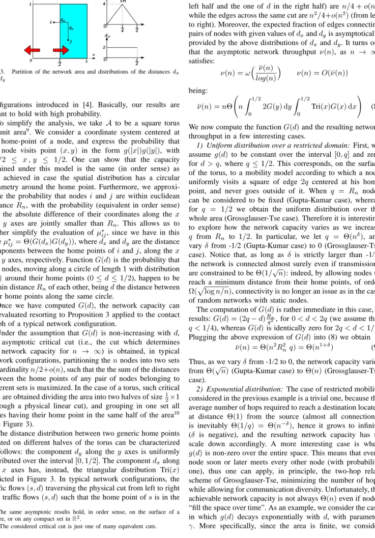
2 1 2 1 2 1 0 0 dx 0 y d dx dy Tri 1 y x 1 i j 1 4 4 2
Fig. 3. Partition of the network area and distributions of the distances d x
anddy
configurations introduced in [4]. Basically, our results are meant to hold with high probability.
To simplify the analysis, we take A to be a square torus
of unit area9. We consider a coordinate system centered at
the home-point of a node, and express the probability that the node visits point (x;y) in the form g(jxj)g(jyj), with 1=2 x;y 1=2. One can show that the capacity
obtained under this model is the same (in order sense) as that achieved in case the spatial distribution has a circular symmetry around the home point. Furthermore, we approxi-mate the probability that nodesi andj are within euclidean
distance R
n, with the probability (equivalent in order sense)
that the absolute difference of their coordinates along the x
and y axes are jointly smaller than R
n. This allows us to
further simplify the evaluation of
ij, since we have in this
case ij =(G(d x )G(d y )), whered xand d
y are the distance
components between the home points ofi andj, along the x
andy axes, respectively. FunctionG(d)is the probability that
two nodes, moving along a circle of length1with distribution g(d) around their home points (0d1=2), happen to be
within distanceR
nof each other, being
dthe distance between
their home points along the same circle.
Once we have computed G(d), the network capacity can
be evaluated resorting to Proposition 3 applied to the contact graph of a typical network configuration.
Under the assumption that G(d) is non-increasing with d,
the asymptotic critical cut (i.e., the cut which determines the network capacity for n ! 1) is obtained, in typical
network configurations, partitioning thennodes into two sets
of cardinalityn=2+o(n), such that the the sum of the distances
between the home points of any pair of nodes belonging to different sets is maximized. In the case of a torus, such critical cuts are obtained dividing the area into two halves of size1
2 1
(through a physical linear cut), and grouping in one set all nodes having their home point in the same half of the area10 (see Figure 3).
The distance distribution between two generic home points located on different halves of the torus can be characterized as follows: the componentd
y along the
y axes is uniformly
distributed over the interval[0;1=2℄. The componentd xalong
the x axes has, instead, the triangular distribution Tri(x)
depicted in Figure 3. In typical network configurations, the traffic flows(s;d)traversing the physical cut from left to right
(i.e. traffic flows(s;d)such that the home point ofsis in the 9The same asymptotic results hold, in order sense, on the surface of a
sphere, or on any compact set inR 2
.
10The considered critical cut is just one of many equivalent cuts.
left half and the one of din the right half) are n=4+o(n),
while the edges across the same cut aren 2
=4+o(n 2
)(from left
to right). Moreover, the expected fraction of edges connecting pairs of nodes with given values ofd
xand d
yis asymptotically
provided by the above distributions of d x and
d
y. It turns out
that the asymptotic network throughput (n), as n ! 1,
satisfies: (n)=! (n) log(n) (n)=O((n)) being: (n)=n n Z 1=2 0 2G(y)dy Z 1=2 0 Tri(x)G(x)dx ! (8) We now compute the functionG(d)and the resulting network
throughput in a few interesting cases.
1) Uniform distribution over a restricted domain: First, we assume g(d) to be constant over the interval [0;q℄ and zero
for d>q, where q 1=2. This corresponds, on the surface
of the torus, to a mobility model according to which a node uniformly visits a square of edge 2q centered at his home
point, and never goes outside of it. When q = R
n nodes
can be considered to be fixed (Gupta-Kumar case), whereas for q = 1=2 we obtain the uniform distribution over the
whole area (Grossglauser-Tse case). Therefore it is interesting to explore how the network capacity varies as we increase
q from R n to
1=2. In particular, we let q = (n Æ
), and
vary Æ from -1/2 (Gupta-Kumar case) to 0 (Grossglauser-Tse
case). Notice that, as long as Æ is strictly larger than -1/2,
the network is connected almost surely even if transmissions are constrained to be(1=
p
n): indeed, by allowing nodes to
reach a minimum distance from their home points, of order
( p
logn=n), connectivity is no longer an issue as in the case
of random networks with static nodes.
The computation ofG(d)is rather immediate in this case, It
results: G(d)=(2q d) Rn
q 2, for
0<d<2q (we assume that q<1=4), whereasG(d)is identically zero for2q<d<1=2.
Plugging the above expression ofG(d) into (8) we obtain (n)=(n 2 R 2 n q)=(n 1+Æ ) (9)
Thus, as we varyÆfrom -1/2 to 0, the network capacity varies
from ( p
n) (Gupta-Kumar case) to(n) (Grossglauser-Tse
case).
2) Exponential distribution: The case of restricted mobility considered in the previous example is a trivial one, because the average number of hops required to reach a destination located at distance (1) from the source (almost all connections)
is inevitably (1=q) = (n Æ
), hence it grows to infinity
(Æ is negative), and the resulting network capacity has to
scale down accordingly. A more interesting case is when
g(d) is non-zero over the entire space. This means that every
node soon or later meets every other node (with probability one), thus one can apply, in principle, the two-hop relay scheme of Grossglauser-Tse, minimizing the number of hops while allowing for communication diversity. Unfortunately, the achievable network capacity is not always(n)even if nodes
“fill the space over time”. As an example, we consider the case in which g(d) decays exponentially with d, with parameter . More specifically, since the area is finite, we consider
the truncated exponentialg(d)=e d =(2(1 e =2 )). The complete expression ofG(d)is G(d)= e (d+Rn) [e (e 2Rn 1)(1+d)+ 4(e =2 1) 2 +e (d Rn) (2R n d+3)+e (d+Rn) (2R n +d 3)℄
Substituting the above expression into (8) we obtain
(n)= n 2 R 2 n
which is formally identical to (9) provided that=1=q. Thus,
by letting1==n Æ
, with 1=2<Æ<0, we obtain a network
capacity(n 1+Æ
).
We have repeated the computation in case of a truncated Pareto distribution defined over [R
n
;1=2℄, obtaining a
simi-lar continuous variation of network capacity in between the extreme cases of Gupta-Kumar and Grossglauser-Tse as we vary the mean value ofg(d), this time through the power-law
exponent.
3) Uni-dimensional mobility: Quite surprisingly, a network capacity of (1) can be sustained even when nodes visit
a small fraction of the entire network area. This has been already pointed out in [4], where the authors assume that nodes are constrained to move just along uni-dimensional paths. Our framework allows to recover and extend this result in a simple way. For simplicity, we assume that nodes are constrained to move either on a vertical or horizontal path (each with probability 1/2) passing through their home-point. As opposed to the uniform assumption adopted in [4], we allow the nodes to visit the points along their path according to a given distribution g(d) of the distance from the home
point, which is assumed to be non-increasing with d. The
dominant contribution to network capacity is provided by communication links between nodes moving along orthogonal directions. Actually, contacts between a horizontal (vertical) node i and a vertical (horizontal) node j, occur only when
both nodes simultaneously fall within distance R
n from the
unique intersection point between their paths (see Fig. 3). Hence the capacity
ij
of communication link(i;j), is ij = (g(d x )g(d y )R 2 n
), where the distributions of d x and
d y are
those reported in the right of Figure 3. Considering thatG(d)
is(g(d)R n
), and that the number of edges across the critical
cut isn 2
=8+o(n 2
), by comparing with (8) we recognize that
(n) is the same as that achieved under a two-dimensional
mobility pattern having the same distance distribution g(d)
along the two dimensions.
This fact allows us to make an interesting observation. Suppose that nodes are constrained to visit uniformly a fraction
n
of the space, with1=2< <1, over a rectangular domain
of minimum edge equal to n 1
2, and random orientation. It
turns out the the best solution in terms of network capacity is to stretch out the domain as much as possible, forming a rectanglen 1 2 n 1 2
, which achieves a capacity n 3 2
. The worst case instead is the square of edgen
2, which achieves
a capacity n 1
2. We conclude that the network capacity is
significantly affected by the shape of the domain visited by the nodes. In this sense, uni-dimensional mobility over maximum
length paths (as in [4]) can be considered to be a best-case scenario.
4) Multiple classes of nodes: Our technique based on the application of Proposition 3 over the typical contact graph provides quite a powerful and flexible tool to evaluate the network capacity in very general conditions. In particular, we can also mix different classes of users with different mobility patterns. As an example, we consider the case of
n
nodes visiting uniformly the entire area (class A nodes), with 0 < < 1; the remainingn n
nodes (class B) are assumed to move around a randomly located home-point with distributiong(d). The average ofg(d)is(n
Æ
), (Æ<0), as in
the previously considered examples. To evaluate the network capacity, we consider that the critical cut is traversed by:
n 2 =4+o(n 2 )edges of capacity( 1 n
)(among nodes of class
A), (n n ) 2 =4+o((n n ) 2 ) edges of capacity (n Æ 1 )
(among nodes of class B), andn (n n )=2+o(n (n n )) edges of capacity ( 1 n
) (cross capacity A-B). We obtain a
network capacity (n) =(n
+n 1+Æ
). Thus, to have any
impact on network capacity (in order sense), the fraction n
of fully mobile nodes of classA must satisfy >Æ+1.
V. CONCLUSIONS
In this paper we have considered an ad hoc wireless network composed of n heterogeneous mobile nodes and proposed a
general methodology that allows to precisely characterize its capacity region by considering the associated contact graph, highlighting several important structural properties of the system. We have, then, extended our study to the asymptotic regime (for n ! 1) and obtained fundamental results of
general validity. Finally we have computed the asymptotic capacity of an ad-hoc network under significant examples of non-uniform mobility models of the nodes. Our results show that under anisotropic mobility patterns network capacity may vary with continuity from(
p
n)(Gupta-Kumar case) to (n) (Grossglauser-Tse case).
REFERENCES
[1] P. Gupta, P.R. Kumar, “The capacity of wireless networks”, IEEE Trans.
on Information Theory, vol. 46, n.2, pp. 388–404, Mar. 2000
[2] M. Grossglauser, D.N.C. Tse, “Mobility increases the capacity of ad hoc wireless networks”, IEEE Trans. on Networking, vol. 10, n.2, pp. 477–486, Aug. 2002
[3] P. Hui, A. Chaintreau, J. Scott, R. Gass, J. Crowcroft, C. Diot, “Pocket Switched Networks and the Consequence of Human Mobility in Con-ference Environments”, ACM WDTN, Philadelphia, PA, Aug. 2005 [4] S.N. Diggavi, M. Grossglauser, D.N.C. Tse, “Even one-dimensional
mo-bility increases ad hoc wireless capacity”, IEEE Trans. on Information
Theory, vol. 51, n. 11, pp. 3947–3954, Nov. 2005
[5] S. Toumpis and A. Goldsmith, “Large wireless networks under fading, mobility, and delay constraints”, IEEE INFOCOM, Hong Kong, China, Mar. 2004
[6] A. El Gamal, J. Mammen, B. Prabhakar, and D. Shah, “Throughput-Delay Trade-off in Wireless Networks”, IEEE INFOCOM, Hong Kong, China, Mar. 2004
[7] G. Sharma, R. R. Mazumdar and N. B. Shroff, “Delay and Capacity Trade-offs in Mobile Ad Hoc Networks: A Global Perspective” IEEE
INFOCOM, Barcelona, Spain, Apr. 2006
[8] A. Al Hanbali, A. A. Kherani, R. Groenevelt, P. Nain, E. Altman, “Impact of Mobility on the Performance of Relaying in Ad Hoc Networks,” IEEE
INFOCOM, Barcelona, Spain, Apr. 2006
[9] J. Mammen, D. Shah, “Throughput and Delay in Random Wireless Networks: 1-D Mobility is Just As Good As 2-D”, IEEE ISIT, Chicago, IL, July 2004
[10] R. M. Moraes, H. R. Sadjadpour and J. J. Garcia-Luna Aceves, “Mobility-Capacity-Delay Trade-off in Wireless Ad Hoc Networks,” Elsevier
Journal on ad hoc networks, July 2005
[11] Delay Tolerant Network Research Group (DTNRG):www.dtnrg.org
[12] S. R. Kulkarni, P. Viswanath, “A Deterministic Approach to Throughput Scaling in Wireless Networks,” IEEE Trans. on Infornation Theory, vol. 50, no. 6 , pp. 1041–1049, June 2004
[13] S. Toumpis, “Capacity bounds for three classes of wireless networks: asymmetric, cluster, and hybrid”, ACM MobiHoc, pp. 133–144, Tokyo, Japan, May 2004
[14] R. Madan, D. Shah, “Capacity-Delay Scaling in Arbitrary Wireless Net-works”, Allerton Conference, Monticello, IL, 2005
[15] U. C. Kozat and L. Tassiulas, “Throughput capacity of random ad hoc networks with infrastructure support” ACM MobiCom, pp. 55–65, San Diego, CA, Sep. 2003
[16] A. Agarwal and P. R. Kumar, “Capacity bounds for ad-hoc and hybrid wireless networks”, ACM Computer Communications Review, vol. 34, no. 3, pp. 71–81, July 2004
[17] B. Liu, Z. Liu, and D. Towsley, “On the capacity of hybrid wireless networks”, IEEE INFOCOM, vol. 2, pp. 1543–1552, San Francisco, CA, Apr. 2003
[18] S. R. Kulkarni, A. Reznik and S. Verd´u, “A “Small World” Approach to Heterogeneous Networks,” Commun. Inf. Syst., vol. 3, no. 4, pp. 325– 348, Sep. 2004
[19] L. Fratta, M. Gerla, L. Kleinrock, “The Flow Deviation Method - An Approach to the Store-and-Forward Communication Network Design,”
Networks, vol. 3, pp. 97-133, 1973
[20] M. Bramson, “Convergence to Equilibrium for Fluid Models of FIFO Queueing Networks”, Queueing Systems, vol. 22, pp. 5-45, 1996 [21] Y. Aumann and Y. Rabani, “AnO(logk)Approximate Min-Cut
Max-Flow Theorem and Approximation Algorithm”, SIAM Journal on
Com-puting, vol. 27, n. 1, 1998
[22] P. Hall.“Introduction to the Theory of Coverage Processes,” John Wiley & Sons, New York, 1988
APPENDIXI PROOF OFTHEOREM3
In a network comprisingn nodes, consider a pair (i;j)2 (t) and draw a circle of radius r
i
= d
ij
(t) around the
transmitter node i; by construction, according to the
inter-ference model, no other transmitting node k can lie in the
circle (otherwise it would cause interference at receiver j).
Draw now a circle of radiusr i
=2around every simultaneously
transmitting nodei; by construction, all these circles cannot
overlap at any point. Thus:
X (i;j)2 (n) (t) 2 4 d 2 ij 1
and for any value n >0, by simple inequality, X (i;j)2 (n) (t) 2 n I d ij > n X (i;j)2(t) d 2 ij 4 2
thus dividing both size by(n)we obtain: 1 (n) X (i;j)2 (n) (t) I d ij (t)> n 4 2 n (n) 2
Integrating both sides and dividing byt: 1 (n)t Z t 0 X (i;j)2 (n) () I d ij ()> n d 4 2 n (n) 2
By makingt!1, for ergodicity, we obtain: 1 (n) X (i;j)2 (n) (t) E[I dij(t)>n ℄ 4 2 n (n) 2 At last, for n!1, if n =( 1 p (n) ): limsup n!1 1 (n) E h X (i;j)2 (n) (t) I dij()>n i =0
i.e., asymptotically the fraction of traffic transported over link with length n =( 1 p (n) )is negligible. APPENDIXII PROOF OFTHEOREM4 The proof goes through four main steps.
Step 1. Extending standard coverage results [22] under the assumption of independence and the assumption that
inf X
(X) > 1
> 0, it is possible to prove that with
probabilityp(n)>1 1=n 2
, all points ofAfall within at least
one of the circles centered at network node locations of radius
a(n)= 4logn
n
. In such a case we say thatA is fully covered.
As a consequence, with probabilityp(n), between any pair of
nodes, i and j such that d ij
> 4a(n), an ordered set (finite
chain)C=( 1 =i; 2 ;::: ; h
=j)of intermediate nodes can
be found such that: (a) the maximum distance between nodes inCand the segment connectingitojis not larger thana(n);
(b) the distance between nodes i and
i+1 is not smaller than 2a(n) and is not larger than 4a(n). Note that, neglecting for
the moment the effects of the interference, a connected path can be established along C by selecting a transmission range r(n)=4a(n).
Consider the vector of positions X (n)
and define the sets
B n i;j;C
for any pair of nodes (i;j) and any ordered chain of
nodes C =( 1
=i;:::; h
=j) according to the following
rule: X (n) 2B n i;j;C if d ij
>r(n)=4a(n); then, C forms a
chain satisfying constraints (a) and (b). We define B
n i;j;;
according to the following rule: X (n) 2 B n i;j;; , if d ij
> r(n) = 4a(n) and no chain can be found
satisfying constraints (a) and (b). Finally we denote withB n ; = [ i;j B n i;j;; .
We can restate step 1 saying that the probability that X (n)
falls insideB n ;
is not greater than1 p(n).
Step 2. When X
(n) 2 B
n i;j;C
according to the interference model not all the transmissions (
i ;
i+1
)can simultaneously
occur because of the interference. However, since by construc-tion distance d
ii+1 satisfies:
r(n)=2 d ii+1
r(n), the
transmissions along C can be partitioned into a superposition
of at most d3+2emaximal non interfering sets. This can
be easily proved through elementary geometrical arguments. Step 3. Note that transmission(i;j)completely covers
trans-missions ( i
; i+1
). interfering with all ( i
; i+1
). In addition
transmissions not interfering with (i;j), by construction, do
not interfere with any of ( i
; i+1
)too.
Step 4. Now, given any sequence of scheduling policies
S(n)sustaining a per-node throughput((n))and
employ-ing transmissions with ranges greater than r(n), we show
that a sequence of policies S 0
(n) can be defined sustaining
the same asymptotic throughput but forcing all transmissions ranges to be less or equal to r(n). Note that without lack of
generality we expect the network throughput(n)to satisfies: (n
1 p
First, defining with C S(n);;
the global transport capacity achieved byS(n)whenX(t)2B n ; , it results: C S(n);; =E h X i;j I (i;j)2 S(n) (t);X(t)2B n ; i nPrfB n ; g= 1 n
where the inequality derive by the fact that by construction
j S(n)
(t)j n. Thus asymptotically the global transport
capacity of C S(n);;
(i.e. the information that flow through
C S(n);;
) is negligible with respect to the network throughput. As a consequence we can define a sequence of policiesS
0 (n)
which differ fromS(n)becauseS 0
(n)mapsX(t)2B n ;
into
(t) = ;, and conclude that the sequence of policies S 0
(n)
achieves asymptotically the same throughput ofS(n).
Policies S 0
(n) are obtained by modifying policies S 0
(n)
according the following rule: whenever X(t) 2 B n i;j;C and (i;j) 2 S(n) (t), S 0 (n) (t) differs from S 0 (n) (t) because (i;j) is substituted by a randomly selected maximal set of
non interfering transmissions alongC; this is possible thanks to
arguments in Step 3. Note that thanks to Step 2, the probability of selecting any transmission along C is greater or equal to 1=(2+2). LetC S(n);d ij >r(n);C ij
denote the capacity exploited byS 0
(n)
on link (i;j)when X(t)2B n i;j;C , by construction C S 0 (n);d ij >r(n);C ij =E[I (i;j)2 S 0 (n) (t);X(t)2B n i;j;C ℄ LetC S 0 (n);d ij >r(n) ij
denote the capacity exploited byS 0
(n)
on link (i;j)when d ij >r(n) C S 0 (n);dij>r(n) ij = X C6=; E[I (i;j)2 S 0 (n) (t);X(t)2B n i;j;C ℄+ E[I (i;j)2 S 0 (n) (t);X(t)2B n i;j;; ℄= X C6=; C S(n);d ij >r(n);C ij by constructionS 0 (n)replaceC S(n);dij>r(n);C ij with capacities along chainC; letC
S 0 (n);d ij >r(n);C ij
be the extra capacity along
C provided byS 0 (n)(with respect toS 0 (n)); it results: C S 0 (n);d ij >r(n);C ij 1 3+2 C S(n);d ij >r(n);C ij
Summing over all possible chains C, it follows that a finite
fraction of the removed capacity between(i;j),C S(n);d ij >r(n) ij is reestablished byS 0
nalong all chainsC.
Thus sequence of S 0
(n) asymptotically achieves the same
throughput ofS 0
(n)andS(n).
At last we notice that arguments used in this proof are rather conservative; in general we may expectS
0
(n)to achieve better
asymptotical throughput properties ofS(n)in light of the fact
long range transmission (i;j) can be replaced in S 0
(n) not
just with transmission along chainC. Many other short range
transmissions falling within the transmission range of (i;j)
are possible in S 0
(n).
APPENDIXIII
PROOF OFTHEOREM5
First we prove that for eachiandj, (n) ij =(Prfd (n) ij p n g). Indeed, by construction: Prfd (n) ij p n g= Z Xi2A Z Xj2B(Xi;= p n) dF (n) j (X j )dF (n) i (X i )
while, by restricting the integration domain in (7):
(n) ij 1 2 Z X i 2A Z X j 2B(X i ;= p n) h Y k 6=i;j Z X2A(Xi;Xj) dF (n) k (X) i dF (n) j (X j )dF (n) i (X i ) (10)
Thus to prove the assert, it is sufficient to show that
lim n!1 Q k 6=i;j E[I X (n) k (t)2A(Xi;Xj)
℄ > a.e. for some > 0. Note that lim
n!1 E[I X (n) i (t)2B(X0;= p n) ℄ represents
the limiting probability of finding mobile i at location X 0,
i.e., by ergodicity, the limiting fraction of time that mobile i
spends still at locationX
0. By construction, excluding at most
a denumerable set of points fX m g, 8X 0 2=fX m g, it results: lim n!1 E[I X (n) i (t)2B(X0;= p n) ℄ = 0. Thus fixing X i with X i 6=X m, considering X j 2B(X i ;= p
n)and defining for
short: p n k = 1 E[I X (n) k 2A (X i ;X j ) ℄, we have: p n k ! 0, for
anyk whenn!1. Thanks to (6): lim n!1 n X k =1 p n k <+1 (11)
The assert is proved if we show that:lim n!1 Q n k =1 (1 p n k )> >0. By the continuity oflogfunction, this is equivalent to:
lim n!1 n X k =1 log (1 p n k )>log> 1 (12)
Observe that log(1 x) > 2x for any 0 x x 0, with x 0 0:8 such that 1 x 0 = exp( 2x 0
), and that for n
sufficiently large we can assume p n i
<x
0; thanks to (11) we
can easily show (12).
At last, to prove that S
selects w.h.p. transmission ranges which are O(1=
p
n) it is sufficient to show that lim n!1 Q k 6=i;j E[I X (n) k (t)2A (X i ;X j ) ℄=0wheneverd (n) ij = !( 1 p n
). Also in this case, defining for short: p n k = 1 E[I X (n) k 2A(Xi;Xj) ℄ it results: lim n!1 P n k =1 p n k = +1. Since log(1 x) x: lim n!1 n X k =1 log(1 p n k ) n X k =1 p n k = 1
and thus by continuity of exponential function:
lim n!1 Q n k =1 (1 p n k )=0.