Contents lists available atScienceDirect
Computers and Mathematics with Applications
journal homepage:www.elsevier.com/locate/camwaMulti-thread implementations of the lattice Boltzmann method on
non-uniform grids for CPUs and GPUs
M. Schönherr
∗, K. Kucher, M. Geier, M. Stiebler, S. Freudiger, M. Krafczyk
TU Braunschweig, Institute for Computational Modeling in Civil Engineering (iRMB), 38106 Braunschweig, Germany
a r t i c l e i n f o Keywords: Multi-core Multi-scale Lattice Boltzmann GPU
a b s t r a c t
Two multi-thread based parallel implementations of the lattice Boltzmann method for non-uniform grids on different hardware platforms are compared in this paper: a multi-core CPU implementation and an implementation on General Purpose Graphics Processing Units (GPGPU). Both codes employ second order accurate compact interpolation at the interfaces, coupling grids of different resolutions. Since the compact interpolation technique is both simple and accurate, it produces almost no computational overhead as compared to the lattice Boltzmann method for uniform grids in terms of node updates per second. To the best of our knowledge, the current paper presents the first study on multi-core parallelization of the lattice Boltzmann method with inhomogeneous grid spacing and nested time stepping for both CPUs and GPUs.
©2011 Elsevier Ltd. All rights reserved.
1. Introduction
Strategies for the efficient implementation of computationally intensive numerical methods, such as the lattice Boltzmann method for the simulation of fluid flow, have to address specific properties of the latest hardware. Currently, this development is focused on systems with an increasing number of computational units within one die. These systems emerge not only in the form of multi-core CPUs, but also as special multi-processing units with a particularly large numbers of cores. Noteworthy among these are the General Purpose Graphics Processing Units (GPGPUs), due to their high performance to price ratio. For example, the recently released nVIDIA TESLA C1060 has been observed to deliver about 5
·
1011single precision(32 bit) floating point operations per second (0.5 TFLOPS), while the theoretical peak performance of the Intel Core2 Quad Q8200 2.38 GHz is only 38 GFLOPS for double precision and 76 GFLOPS for single precision. Also, the bandwidth of the memory interface is 102 GB
/
s for nVIDIA’s TESLA C1060 and is thus much larger than the bandwidth of a desktop computer (up to 17,
06 GB/
s for DDR3—double channel memory). On the other hand, GPGPUs are not as flexible as CPUs with regard to the layout of data structures, thus efficient computation on GPGPUs requires structured data.The lattice Boltzmann algorithm is especially suitable for implementation on GPGPUs [1,2] due to its utilization of Cartesian grids and its typical restriction to next neighbor communication between lattice nodes. However, the usage of uniform Cartesian grids is expensive, as the complete computational domain has to be discretized with the same resolution irrespective of the local geometric and fluid dynamic complexity. Although scientific problems exist for which a homogeneous description of the domain is a reasonable choice (such as flow in porous media), it is usually desirable to resolve regions of high geometrical complexity with a finer grid than is used for peripheral regions of the flow field. It is possible to change the resolution in the lattice Boltzmann method, provided that suitable interface conditions are imposed between the regions of different resolutions. The interface conditions and the utilization of multiple grid levels add complexity to the original lattice Boltzmann method and, consequently, make the implementation on highly structured
∗Corresponding author.
E-mail address:[email protected](M. Schönherr). 0898-1221/$ – see front matter©2011 Elsevier Ltd. All rights reserved. doi:10.1016/j.camwa.2011.04.012
computational hardware such as GPGPUs more challenging. In this paper, we investigate and compare two multi-thread parallel implementations of the multi-scale lattice Boltzmann method. The first implementation is done for a multi-core CPU system in an object oriented framework. The second implementation is done for a GPGPU using the CUDA SDK [3] and is based on the code discussed in [1]. For grid refinement, both codes use the compact second order accurate interpolation technique introduced in [4].
2. The multi-scale lattice Boltzmann equation
The lattice Boltzmann equation for fluid dynamics is derived from the continuous Boltzmann equation, which describes the probability of finding a fluid particle in a certain velocity state at a certain position and time [5,6]. The lattice Boltzmann equation is a simplification of the Boltzmann equation, allowing particle distributions to move only within a small set of discrete velocities. Commonly used sets are 9 velocities in two dimensions and 13, 15, 19, or 27 velocities in three dimensions. The naming convention of lattice Boltzmann velocity sets by Qian [7] isDdQq, withdbeing the number of dimensions andqbeing the number of discrete velocities, respectively. In this paper, we consider the two-dimensional D2Q9 velocity set. The primitive data structure for the lattice Boltzmann equation consists of a Cartesiand-dimensional field of lattice nodes. Each lattice node holdsqdiscrete populationsfiassociated with theqdifferent velocities. The set of velocities
is chosen such that, after one time step1t
=
1 (in reduced units), each populationfihas moved along the vectorei1tto aneighboring lattice node. In the case of the D2Q9 lattice, four populations move to neighbors along the primary axes, four populations move along the diagonals, and one population remains on the lattice node. The propagation of populations is followed by the collision step, which is typically a function that depends only on the nine local populations at the given time step. It conserves the zeroth and the two first statistical moments of the local distribution of populations, corresponding to mass and momentum, and relaxes the higher moments toward an equilibrium state (typically taken as a Taylor expansion of a Maxwellian). Hence, the lattice Boltzmann equation can be written as:
fi
(
x+
ei1t,
t+
1t)
−
fi(
x,
t)
=
Ω(
fi(
x,
t)).
(1)For simplicity, the collision operatorΩ
(
fi(
x,
t))
in this study is the BGK or single relaxation time type approach [8]:Ω
(
fi(
x,
t))
= −
∆tτ
fi(
x,
t)
−
f eq i(
x,
t)
.
(2)The equilibrium distribution for the standard BGK model is:
fieq
=
w
iρ
1+
3(
ei·
u)
c2+
9 2(
ei·
u)
2 c4−
3 2 u2 c2
(3) withc=
1x/
1tbeing the particle velocity in the primary lattice directions,w
ibeing the weights for the different directions,and
ρ
andubeing the macroscopic mass and velocity, respectively. The densityρ
is computed from the zeroth moment of the nodal distribution functionfiand the velocity is obtained from the momentumu=
j/ρ
. Introducing a constant backgrounddensity
ρ0
and redefining the velocity to beu=
j/ρ0
, He and Luo [9] obtained an incompressible lattice Boltzmann method with the equilibrium function:fieq
=
w
iδρ
+
w
iρ0
1+
3(
ei·
u)
c2+
9 2(
ei·
u)
2 c4−
3 2 u2 c2
.
(4)Incompressibility of the model is obtained only for steady state solutions. However, one distinguishing property of this model is that only the density fluctuations
δρ
have to be stored in memory. These values fluctuate around zero and better use is made of the available digits of floating point numbers than in the standard model. The only material parameter in the model defined by(1)and(2)is the kinematic viscosityν
, which is controlled by the relaxation timeτ
in the collision operator. Asymptotic analysis of the lattice Boltzmann equation shows that it generates the solution of the incompressible Navier–Stokes equation for the low order moments in the limit of small grid spacings and time steps [10] where viscosity is related to the relaxation time asν
=
2τ
−
16
1x2
1t
.
(5)Although the standard LBM does not permit a continuous change in grid resolution, it is still possible to change the resolution arbitrarily, provided that suitable interface conditions are imposed between regions of different resolutions. The computational complexity of the interface condition is typically reduced by allowing only integer ratios of grid spacing and time step length between neighboring areas with different resolutions. The simplest method of grid coupling, which we adopt here, uses a grid spacing ratio of1xc
/
1xf=
2 where1xcand1xfare the grid spacings in the coarse and fine grids,respectively [11,12]. For time step length, acoustic scaling is applied where the time step ratio is proportional to the grid spacing ratio:1tc
/
1tf=
1xc/
1xf.It is also possible to apply the diffusive limit1tc
/
1tf=
(
1xc/
1xf)
2=
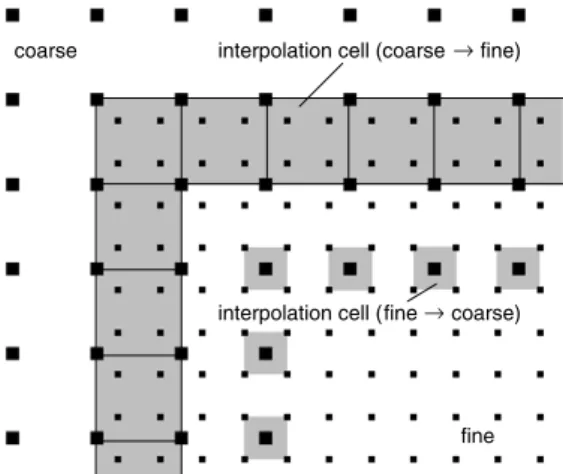
4, which one might assume to be more consistentFig. 1. The overlapping interfaces between a coarse and a fine patch. The lattice nodes in the gray regions are filled with distributions obtained by second order compact interpolation between the four enclosing lattice nodes. The compact interpolation method utilizes the statistical moments of the distribution functions of the four enclosing lattice nodes to compute distributions at the internal nodes.
The acoustic scaling is applied for grid coupling for three reasons. First, the overall convergence of the lattice Boltzmann equation to the Navier–Stokes equation in the diffusive limit is not affected by this choice of interface conditions. Second, diffusive scaling would reduce errors in the Mach number and the grid spacing in the refined regions as compared to the coarse regions. The acoustic scaling keeps the Mach number identical in both regions. Hence, Mach number errors are not reduced in the fine region as compared to the coarse region. In exterior flow problems, finer grids are typically applied close to the regions of high geometric complexity near the boundaries. Here, the purpose of grid refinement is to reduce errors in grid spacing. Close to the surface of the body experiencing the flow, the Mach number is usually not larger than far from the body. Allowing a larger error in the Mach number in the coarse regions does not make sense when the Mach number is highest in the coarse regions. Third, since the acoustic scaling leads to identical Mach numbers on fine and coarse grids, the interfacial condition is naturally non-reflective. A sudden change in the Mach number along the interfaces between regions of different resolutions is undesirable, as it imposes an obstacle for pressure waves.
At the interfaces, nodal information has to be interpolated from the coarse grid to the fine grid and from the fine grid to the coarse grid in a synchronization step. To consistently recover the second derivatives of the velocity and the first derivatives of the pressure in the Navier–Stokes equation, we require an interpolation of the velocity field which is at least second order accurate and an interpolation of the pressure field which is at least first order accurate. Since we apply the acoustic scaling by keeping the Mach number constant over the grid interface, the relaxation time
τ
has to be scaled in order to obtain the same Reynolds number on both lattices [11]. In this paper, we adopt a recent approach using second order compact velocity interpolation in a square spanned by four lattice nodes [4]. A naive second order accurate interpolation in two dimensions would require six points which cannot be arranged both symmetrically and compactly on a Cartesian grid. Our symmetric compact interpolation method obtains the missing information from the derivatives of the velocity hidden in the second moments of the nodal distribution function via asymptotic analysis [10]. Two types of interpolation cells are used: fine to coarse interpolation cells and coarse to fine interpolation cells (seeFig. 1). Each cell receives its information from the four nodes at its corners. All nodes enclosed in the interpolation cell are reconstructed from compact interpolation in the synchronization step. Synchronization happens every coarse time step (i.e., every two fine time steps).Time interpolation is not required in this method since the fine grid reaches two lattice spacings into the coarse domain. Hence, the fine domain is enclosed in two rings of interpolated fine grid nodes. The outer ring becomes invalid in the asynchronous time step. Both rings are refilled immediately after the inner ring becomes invalid. The symmetric interpolation cells make the application of the interface condition independent of the orientation of the interface and does not require any special treatment for corners. The simplicity of the method is a big advantage, especially for the GPGPU implementation where decisions or exceptions would be expensive. The utilization of an overlapping region has to be discussed with regard to efficiency. The outer ring of fine lattice nodes is not really required and can be replaced by interpolation in time between two subsequent coarse time steps. This approach has been discarded here due to the following efficiency considerations: If time interpolation were to be used, the interpolation function would have to be evaluated every fine time step instead of every coarse time step (that is, twice as often as in the current implementation). In order to interpolate in time, two time steps would have to be kept in memory for the interpolation cells. This would require more memory than would be used for storing the outer ring of fine lattice nodes. Further, saving memory by disregarding the outer ring would make the interpolation cells asymmetric. A different treatment for all orientations of the wall would be necessary and corners would be singular exceptions, spoiling parallel efficiency. Therefore, we conclude that the current implementation is conceptually more efficient than a time interpolation technique. Details on the interface conditions are given in [4]. A similar approach can be found in [14].
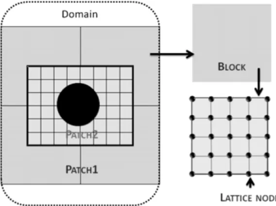
Fig. 2. Data structure for the geometric partitioning of the computational domain. A domain holds the complete simulation. A patch stores the data associated with one threat. A block is a geometric regular subpartitioning of a patch. The lattice nodes provide the atomic data structure of the lattice Boltzmann method.
3. Thread based CPU code
In this section we describe the implementation of the lattice Boltzmann model on a multi-core platform with the computational work assigned to CPUs. Multi-core parallelization strategies for the homogeneous grid lattice Boltzmann method have been studied by Donath et al. [15], Peng et al. [16], and Williams et al. [17]. To the best of our knowledge, the current paper presents the first study on multi-core parallelization of the LBM with inhomogeneous grid spacing and nested time stepping for both CPUs and GPUs. A CPU implementation of the lattice Boltzmann model can take advantage of established programming paradigms and the flexibility of the hardware. Debugging the software, as well as porting the software to other platforms, is substantially simpler than in the case of a special hardware implementation such as the GPGPU code described in the next section.
3.1. Geometric partitioning of the simulation domain
The implementation of the CPU lattice Boltzmann code is based on a hierarchy of geometrical subdivisions of the computational domain that facilitates parallel computations (Fig. 2). These subdivisions can be classified, from the bottom of the hierarchy up, as:
•
lattice node: a geometrical point element that holds one set of distributionsfi.•
block: a set of lattice nodes that are spatially arranged in the form of a rectangular two (2D) or three (3D) dimensionalarray. The individual nodes in a block can be accessed by indices (B
(
x,
y)
orB(
x,
y,
z)
) and the grid spacing between nodes belonging to one block is homogeneous.•
patch: a set of blocks with identical grid resolution connected by at least one block face.•
domain: represents the set of patches that make up the complete geometrical model underlying the physical problem.In what follows, we assume without loss of generality that each thread deals with one patch only. Thus, in our notation, a patch corresponds to what is classically termed a (geometric) subdomain.
Patches may contain subpatches. A patch contained completely in a larger patch is calledchild patchand the patch containing a smaller patch is calledparent patch. Parent and child patches are related by parent-and-child-relations which are determined as part of the pre-processing. Patches sharing a geometrical boundary are related by neighbor-relations. These relationships are required for consistent synchronization. Parent and child synchronizations are applied in the interface condition when the parent and the child have different grid resolutions. Geometrically connected patches with the same resolution require synchronization with their neighbors.
The size of one block (which can be specified by the user) is the smallest unit of grid refinement and the smallest unit of computational load distribution. Lattice node based load balancing would be prohibitive due to the large number of lattice nodes in the computation [18,19] which in three dimensions may exceed 109. The number of blocks is usually more than
three orders of magnitude smaller than the number of lattice nodes. Since blocks are stored in dense multi-dimensional arrays and are being processed one after another in one thread, optimal use of the CPU cache can be made by choosing an appropriate block size.
3.2. Implementation
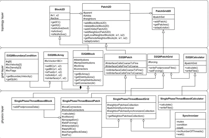
Our implementation is divided into three logic layers [18]: the topology layer, the grid layer, and the physics layer (Fig. A.8
in theAppendix A). The topology layer contains the base classes describing general data structures such as patch, block, and domain.
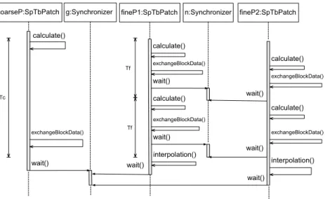
Fig. 3. Synchronization sequence of the patch grid with two resolution levels.1tc=21tf, where1tcis the time step of the coarse patch and1tfis that
of the fine patch.
The grid layer describes the data structures holding the primitive variables of the lattice Boltzmann D2Q9 model. It contains appropriate subclasses of the general data structures and classes specific for this model. Among such classes is the D2Q9BcArray which saves information about lattice node types, i.e. fluid, solid, interface, or boundary condition nodes.
The physics layer implements methods for the specific task set; in this case, it implements the flow simulation for single phase fluid.
The user provides an initial definition of the patches, which is segmented into subpatches according to the number of available compute cores. These subpatches are computed in separate, parallel threads during the simulation. In the current implementation, the assignment task is delegated to the graph based METIS library [20] for automated load balancing. Necessary specific node and edge weights are assigned as described in [18].
During the simulation, the synchronizer class guarantees that the different patches/threads work on consistent data. Two kinds of synchronization have to be distinguished on the patch level: the synchronization between fine and coarse patches along the interface condition (this is the parent–child synchronization) and the synchronization between neighboring patches.Fig. 3shows an example for the synchronization of two neighboring fine patches contained in one coarse patch. This structure naturally allows for an arbitrary deep recursive nesting of grids with different resolutions. The class structure is listed inAppendix A.
4. GPGPU code
A GPGPU based implementation of the lattice Boltzmann method has the potential to run up to one order of magnitude faster than a CPU code due to the large number of cores. The nVIDIA TESLA C1060 GPGPU offers 30 single instruction multiple data processors with eight cores each, resulting in 240 cores. The programming paradigm for these devices differs from CPU programming and is completely focused on parallel execution. Instead of processing data sequentially in loops, the high number of cores allows one to process each lattice node with its own thread. The GPGPU code used here is based on the one presented in [1]. The GPGPU applies a special memory access pattern that has to be taken into account in order to obtain an efficient code. When accessing the main memory, the multi-processors read data in segments of 64 bytes. This data is distributed over 16 simultaneous threads running on the multi-processor, called a warp. The 64 bytes correspond to 16 four byte floating point numbers. In order not to waste bandwidth, the nodes processed by the threads of one multi-processor should be aligned in such a way that they read from consecutive places in the memory. Instead of storing the state vectors node by node, the distributions are stored in arrays according to their lattice direction. The index of the array is aligned in thex-direction. In the streaming step, particle distributions have to move in thex-direction as well as in the
y-direction. Streaming in thex-direction shifts the index of a distribution by one so that the array is misaligned with respect to the segments after streaming. In order to re-align them, we make use of the shared memory that can be accessed by all threads running on one multi-processor. Streaming in thex-direction is done in shared memory first. After synchronization of all of the threads, the distributions are again aligned with the segments and can be written back to main memory by the warps. For streaming in they-direction, the segments are automatically aligned if the first element in each row is aligned with a segment. Since the rows are stored consecutively in the memory, the length of the domain in thex-direction should be a multiple of the 16 lattice spacings. Otherwise, it has to be padded with empty nodes. Streaming in the four diagonal directions is done by first streaming in thex-direction in the shared memory and, after the synchronization, streaming in the alignedy-direction.
The GPGPU code is augmented by the same compact interface condition for grid coupling as the above CPU code. The in-terface condition for the grid refinement uses a pre-computed list of interpolation cells holding the indices of the associated nodes on the fine and coarse grids. Following the new programming paradigm, each entry in the list is assigned to a thread and processed in parallel during the application of the interface condition. Note that by using a list of indices, performance is completely independent of the form and topology of the interface line. It is an essential feature of our implementation that the compact second order interpolation method is independent of the orientation of the interface and does not require a special treatment of the corners. Exceptions like corners are likely to introduce computational overhead that is dispropor-tionate to their frequency of occurrence. For example, if each one of the four corners in the interface of a rectangular block were to require special treatment, they would either have to be processed sequentially in a special step while the rest of the simulation waited or the interface condition would have to check whether an interpolation cell were a corner cell. Both methods would be very expensive and are fortunately not necessary when using the compact interpolation method.
4.1. Limitations for lattice Boltzmann running on GPGPUs
The GPGPU code used in this study differs in several respects from the CPU code. Currently, the GPGPU code uses only a single coarse and a single fine block for multi-scale simulations. A recursive generalization of this algorithm allowing for grid nesting of arbitrary depths is shown inAppendix B. For the GPGPU code, the patch data structure has not yet been adopted. Also, the GPGPU code differs from the CPU code with respect to the accuracy of the no slip boundary conditions. While the CPU code offers simple link based bounce back boundary conditions, as well as second order accurate interpolation bounce back boundary conditions for curved walls, the GPGPU code uses only node based simple bounce back boundary conditions. In the link based bounce back method, the population streaming away from a lattice node returns in the same streaming step to the node from which it came. The node based bounce back method is applied on boundary nodes, replacing the collision step. The population returning from the boundary node arrives one time step later than the population arriving from a link based bounce back boundary condition. Both methods converge to the same steady state and their accuracy is not substan-tially different, since the lattice Boltzmann method itself is only first order accurate in time. The motivation for implementing a node based bounce back boundary condition is that node based boundaries are independent of the orientation of the wall. This simplifies their implementation. The reason for the simpler structure of our GPGPU code, as compared to the CPU code, is only partially motivated by the restrictions of the new programming paradigm. The primary reason is that at the time of this writing, substantially more person hours have been invested in the development of the CPU code than in the GPGPU code. The GPU code uses single precision floating point numbers whereas the CPU code uses double precision. As a result, the impact of single precision accuracy on the lattice Boltzmann method will be discussed in detail in the following subsection.
4.2. Single precision floating point numbers
The impact of the reduced numerical precision on lattice Boltzmann simulations due to the usage of 32 bit floating point numbers, as compared to 64 bit floating point numbers, has been investigated by Harvey et al. [21] using a cell processor implementation. They concluded that single precision was sufficient for test cases but they observed some loss in mass and momentum over time. This violation of the conservation laws could be traced back to the fact that the cell processor always rounds the fraction of the floating point number to the next lower value. Since the distribution functions in the standard lattice Boltzmann model are always positive, rounding down must result in loss of mass. No such violation of the conservation laws was observed when compared to architectures that rounded to the nearest even value. We note here that our GPGPU platform supports rounding to nearest even value.
A single precision IEEE 754 floating point number consists of 32 bits: one for the sign, eight for the exponent, and 23 for the fraction. This compares to a double precision number having one bit for the sign, eleven bits for the exponent, and 52 bits for the fraction. In both cases, the fraction also contains a hidden bit since the leading digit of a binary floating point number is always one. Hence, the range of the fraction of a single precision number is 24 bits long. The variables used in the lattice Boltzmann method are the populationsfi. Thefican be decomposed into equilibrium and non-equilibrium parts fi
=
fieq+
fneq
i . The equilibrium part is a function of the conserved quantities
ρ
anduand is given in Eq.(3)for the standardmodel and in Eq.(4)for the incompressible model.
Scientific conclusions based on computer simulations should only be drawn if the convergence of the simulation results can be established. In the case of the lattice Boltzmann method, convergence is obtained if the results do not change under diffusive scaling, that is when Mach number and grid spacing are reduced proportionally for a fixed Reynolds number. However, the influence of finite numerical precision is expected to increase for smaller Mach numbers and convergence might be lost. In the diffusive scaling, the velocitiesushrink linearly with grid spacing and the local variations in density
δρ
shrink quadratically with grid spacing when mapped to constant physical velocities and densities, respectively. Numerical difficulties arise from the fact that the background densityρ0
is independent of the grid spacing. Here, we use a tilde for the fixed scale quantities as they appear if they are written in SI units. The lattice Boltzmann variables without a tilde are then scaled with the grid spacing:u=
1xu˜
andρ
=
ρ0
+
δρ
= ˜
ρ0
+
12x
δ
ρ
˜
. The standard equilibrium (Eq.(3)) becomes: fieq=
w
i(
ρ0
˜
+
1x2δ
ρ)
˜
1+
31x(
ei· ˜
u)
c2+
9 21x 2(
ei· ˜
u)
2 c4−
1x 23 2˜
u2 c2
.
(6)According to the theory of asymptotic analysis [10], the solution of the lattice Boltzmann method should become more accurate for smaller1x. This applies to all asymptotic errors, such as the non-Galilean invariance of the viscosity. Asymptotic errors decrease with a higher resolution and a lower Mach number. Round-off errors, on the other hand, increase with a lower Mach number (a low Mach number corresponds to a short physical time step). It is observed thatfeqis constant and non-zero toO
(
1x0)
. As a result, the floating point number has a fixed or only weakly varying exponent and, hence, possessa lower numerical significance than an integer of the same size in bits. This also explains why approaches using integers instead of floating point numbers are usually successful [22]. By decreasing the grid spacing and the Mach number with1x, all nonconstant terms will eventually drop below machine precision. The number of significant bitsNthat remain from the available number of bitsNsingle
=
23 can be computed depending on the Mach number Ma= |u|
/
cswith speed of soundcs
=
1/
√
3 for the linear (NMa) and quadratic (NMa2) terms in the equilibrium. For this, we balance the number of bits used
to store the constant term with the number of bits available for linear and quadratic terms: 1 223
=
3√
3Ma 2NMa (7) 1 223=
Ma2 2∗
2NMa2.
(8) This gives rise to:NMa
= −
log
2−23Ma−1 3√3
log 2 (9) NMa2= −
log
2∗
2−23Ma−2
log 2.
(10)The roots of these functions give us the Mach number below which the respective terms in the equilibrium fall below machine precision. The linear term is below machine precision for Ma
<
2.
3∗
10−8, while the quadratic term is already smaller than machine precision for Ma<
0.
0005. For double precision using 52 bits for the fraction, these values are Ma<
4.
3∗
10−17for the linear term and Ma<
2.
1∗
10−8for the quadratic term. The non-equilibrium part offi, coding the
spatial derivatives of velocity and pressure, depends on the local flow structure. According to the asymptotic analysis, the non-equilibrium part offiscales like the quadratic term in the equilibrium. Hence, there is a substantial threat of the accuracy
of single precision floating point numbers becoming insufficient before convergence in the diffusive limit is obtained using the standard equilibrium. The incompressible equilibrium of Eq.(4)makes better use of the available bits since only the deviations from the background density have to be stored. All the 23 bits are now used to store the linear term in the Mach number while the quadratic term is still stored in the lower significant bits. We can balance this by setting:
3
√
3Ma 223=
Ma2 2∗
2NMa2.
(11) Which leads to:NMa2
= −
log
3∗2−22√3 Ma
log(
2)
.
(12)The quadratic term will now fall below machine precision when Ma
<
1.
2∗
10−6. This is substantially better than the value for the standard equilibrium using single precision, but it is still considerably worse than the standard model using double precision. When double precision is combined with the incompressible equilibrium function, the quadratic term drops below machine precision only for Ma<
2.
3∗
10−15. Since round-off errors and asymptotic errors are very different in nature, it is difficult to establish a strict point where the round-off errors become dominant. We observed significant fluctuations in drag and lift values when using the standard equilibrium at a Mach number ofO(
10−4)
. These fluctuationswere suppressed with the incompressible equilibrium.
5. Validation
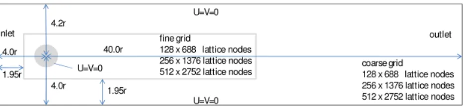
In this section, the multi-core and GPGPU lattice Boltzmann implementations are validated by considering the standard benchmark problems of [23,24]. The test cases are the flow behind a circular cylinder at Reynolds numbers 20 and 100. The benchmark geometry defined by Turek [24] is sketched inFig. 4. The inlet boundary is a parabolic velocity profile. The Reynolds number is defined by
Re
=
u Dν
,
u=
2
Fig. 4. The flow past a cylinder: geometric layout and boundary conditions. The inner rectangle shows the position of the fine grid which has twice the resolution of the coarse grid.
Table 1
Results of drag and lift for compressible and incompressible flows (GPU) and for the compressible model using simple bounce back (SBB) and quadratic bounce back (QBB) boundary conditions at Re=20.
Parameter Incompressible flow (GPU) Compressible flow (GPU) SBB (CPU) QBB (CPU)
Resolution 128×688 nodes cd 5.59242 5.27722 5.5972526 5.5807648 cl 0.0039781 0.0035821 0.0042797 0.0073446 Resolution 256×1376 nodes cd 5.58904 5.41912 5.5870459 5.5731531 cl 0.0090671 0.0085598 0.0162391 0.0101338 Resolution 512×2752 nodes cd 5.59295 5.486955 5.5778068 5.5745483 cl 0.0092500 0.0096763 0.0107031 0.0102097 Table 2
Results of drag and lift for compressible and incompressible flows (GPU) and for the compressible model using simple bounce back (SBB) and quadratic bounce back (QBB) boundary conditions at Re=100.
Parameter Incompressible flow (GPU) Compressible flow (GPU) SBB (CPU) QBB (CPU)
Resolution 256×1376 nodes
cd 3.24188 3.22707 3.261132 3.239529
cl 0.977958 1.00898 1.022869 0.997079
St 0.3 0.3 0.3 0.3
Table 3
Reference values for the flow over a cylinder asymmetrically placed in a channel at Re=20.
Re=20 Present methods Crouse [23] Schäfer and Turek [24] cd 5.49–5.59 5.585–5.627 5.57–5.59
cs 0.0092–0.0107 0.017–0.0119 0.0104–0.011
whereDis the diameter of the cylinder and
ν
is the kinematic viscosity of the fluid. The drag and lift coefficients over the cylinder are computed as follows:cd
=
2Fd
ρ
u2d,
cl=
2Flρ
u2d.
(14)The drag (Fd) and lift forces (Fl) can be obtained by a local exchange of momentum [25]. We simulate this setup with one
level of grid refinement around the cylinder. The fine grid has the same number of nodes as the surrounding coarse grid. For the GPGPU simulations, we compare the compressible and the incompressible model. The multi-core implementation uses the standard compressible model and double precision floating point numbers.
For the curved wall along the cylinder, we compare second order accurate (in grid spacing) bounce back boundary conditions [26,27] to simple link based bounce back boundary conditions for the multi-core code. The GPGPU code currently supports only node based bounce back.
For theRe
=
20 case, we apply diffusive scaling to obtain three different solutions with the resolutions 128×
688, 256×
1376, and 512×
2752 using the inflow velocitiesumax=
0.
0384,
0.
0192, and 0.0096, respectively. The resolutioncorresponds to the coarse outer grid. The fine inner grid has the same number of nodes. The lift and drag coefficients are listed inTable 1.
Periodic vortex shedding is observed atRe
=
100.Table 2lists the maximum ofcd,
cland the Strouhal number obtainedin the simulation by the GPGPU and the multi-core code. The Strouhal number is defined asSt
=
D/
uT. The maximum inlet velocity wasumax=
0.
01 (seeTables 3and4).Table 4
Reference values forcdandclandStfor the flow over a cylinder asymmetrically
placed in a channel at Re=100.
Re=100 Present methods Crouse [23] Schäfer and Turek [24] cd 3.2271–3.2611 3.2645–3.2650 3.22–3.24
cl 0.9780–1.0229 0.9492–1.0709 0.99–1.01
St 0.3 0.3050–0.3076 0.295–0.305
Fig. 5. The performance for different block sizes on different CPUs.
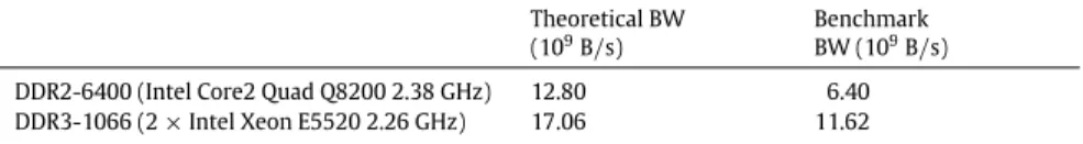
Table 5
Theoretical and measured memory bandwidth of the considered hardware. The benchmark was obtained using STREAM copy [28].
Theoretical BW
(109B/s) BenchmarkBW (109B/s) DDR2-6400 (Intel Core2 Quad Q8200 2.38 GHz) 12.80 6.40 DDR3-1066 (2×Intel Xeon E5520 2.26 GHz) 17.06 11.62
6. Performance analysis
In this section, we investigate the performance of our two codes. We take the number of node updates per second (NUPS) as a general performance measure for the performance of a lattice Boltzmann code and set it in relation to the performance characteristics of the hardware.
6.1. Multi-core code performance
For investigating the performance of the multi-core code, different block sizes have been tested for different CPUs. A two fold periodic uniform system with one million lattice nodes has been simulated to neglect the effects from the boundary conditions and to ensure that each block has the same work load and amount of interblock communication. As shown in
Fig. 5, the optimal block size depends on the CPU being used and its cache size. In general, better results are obtained for smaller blocks starting with 20
×
20 lattice nodes.To determine the parallel efficiency and the scale-up, the same grid was used with a rectangular refinement for the non-uniform setups. In simulations investigating the parallel efficiency, the grid was subdivided into subpatches with METIS to match the number of the available CPU cores. In order to investigate the parallel performance, we conducted measurements for weak scaling with a reference system of two threads and the total system size was a corresponding multiple of 20 million degrees of freedom. For the evaluation of the scale-up, the problem size was linearly increased with the number of threads.
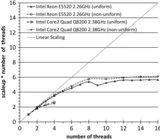
Figs. 6and7show that the parallel efficiency is almost identical for the uniform and the non-uniform grids. The scale-up is indicating that, for a decent number of threads, memory bandwidth ultimately limits the overall performance. The usage of simultaneous multi-threading (more than eight threads on the Xeon processor) leads only to a marginal increase in absolute performance.
In order to confirm that the performance of the multi-core implementation is bandwidth limited, we measure the work done by our code with respect to read and write operations and with respect to floating point operations, and compare it to the performance measures of our computers.Tables 5and6show the theoretical and measured performance of the two computers used in this study. Each lattice population has to be read and written twice: once for collision and once for streaming. The number of bytes to be read and written during the update of one node is:
Fig. 6. The parallel efficiency for uniform and non-uniform computations on different hardware.
Fig. 7. The scale-up for uniform and non-uniform computations on different hardware.
Table 6
Theoretical and measured floating point operations per second (FLOPS) of the considered hardware. Theoretical performance is calculated from the maximal number of operations per cycle and the duration of one circle. The benchmark performance is obtained from a Linpack [29] solving a 1000×1000 linear system.
Cores Theoretical performance FLOPS (×109)
Threads Benchmark performance FLOPS (×109)
Intel Core2 Quad Q8200 2.38 GHz, DDR2-6400
2 19.04 2 1.77
4 38.08 4 3.54
2×Intel Xeon E5520 2.26 GHz, DDR3-1066 4 36.16 4 5.07
8 72.32 8 10.14
Hence, the load bandwidth compares to the peak bandwidth (BW):
LoadBW
=
100%∗
(
NUPS∗
NByte)/
BW.
(16)For the floating point performance, we counted the number of operations in one update step to be NCOLL
=
94. The floating point performance is hence:FPPerformance
=
100%∗
NUPS∗
NCOLL/(
FLOPS∗
number of cores).
(17) Performance measures in terms of bandwidth and FLOPS rate are given inTables 7and8. It is observed that the utilization ratio of bandwidth increases with the number of threads, while the utilization ratio for the available FLOPS rates decreases with the number of threads. Hence, the performance of our code is clearly bandwidth limited.Table 7
Bandwidth utilization of the multi-core code.
Number of threads NUPS (×106) Load of theoretical BW (%) Load of real BW (%)
Intel Core2 Quad Q8200 2.38 GHz, DDR2-6400
2 7.63 17.2 53.7
4 10.7 24.1 75.2
2×Intel Xeon E5520 2.26 GHz, DDR3-1066
4 23.2 39.2 52.4
8 36.6 61.7 73.6
Table 8
Utilization of the floating point capabilities of the multi-core code.
Number of threads NUPS (×106) Theoretical peak performance (%) Real peak performance (%) Intel Core2 Quad Q8200 2.38 GHz, DDR2-6400
2 7.63 3.8 40.6
4 10.7 2.8 29.9
2×Intel Xeon E5520 2.26 GHz, DDR3-1066
4 23.2 6.3 44.8
8 36.6 4.9 35.2
Table 9
Relation of the performance between uniform and non-uniform grids in the GPU implementation. The distinction between raw resolutions includes the nodes of the coarse grid located below the fine patch. The effective resolution excludes the nodes below the fine patch.
Resolution (nodes) NUPS (×106) NUPS (%) time (s/1051t)
Uniform 2048×15 360 911.62 100.00 3450.73 Non-uniform 2×1024×15 360 903.35 99.09 5223.46 (Raw) Non-uniform 2×1024×15 360 828.07 90.84 5223.46 (Effective) −512×7680 Uniform 1024×7680 920.59 100.00 854.27 Non-uniform 2×512×7680 911.20 99.02 1294.6 (Raw) Non-uniform 2×512×7680 835.27 90.73 1294.62 (Effective) −256×3840 Uniform 512×3840 902.55 100.00 217.83 Non-uniform 2×256×3840 837.50 92.79 352.13 (Raw) Non-uniform 2×256×3840 767.71 85.06 352.13 (Effective) −128×1920
6.2. GPGPU code performance
Since the performance of the GPGPU code is expected to depend strongly on the complexity of the algorithm, we have to investigate the impact of the algorithmic overhead due to the employment of non-uniform grids compared to that of uniform grids. We keep the number of degrees of freedom in the uniform case equal to the combined number of degrees of freedom on the fine and the coarse grids in the non-uniform case. All tests are performed using 256 threads per GPU block (a GPU block is the sum of threads run on one multi-processor) and run 100.000 time steps. For the test case with the highest resolution we need about 2.4 GB, for the medium resolution test case about 640 MB, and for the lowest resolution we need about 170 MB of device memory.
The results of our tests are shown inTable 9. We observe that the interpolation at the grid interface is not much more expensive than usual boundary functions, such as inflow and outflow boundary conditions, and decreases the NUPS rate only marginally.
For the raw calculation of the NUPS rate of the non-uniform grid, we consider the entire coarse grid. In the current implementation, the lattice nodes on the coarse grid located ‘‘below’’ the fine grid are not excluded from the calculation. This unnecessary work is currently the only noteworthy overhead in the multi-scale simulation and can be avoided in a refined implementation. InTable 9we thus distinguish between the raw and the effective NUPS rate. The effective number of NUPS excludes the nodes below the fine grid.
7. Conclusion and outlook
In this work, we presented a GPGPU and a multi-core implementation of the LBM for non-uniform grids. The key features leading to an efficient implementation are the multi-level data structures, which allow a seamless transition
Fig. A.8. UML class diagram of the primary data structures in our lattice Boltzmann code. The geometric subdivision in patches and blocks exists on all the three implementation layers.
from block structured to almost unstructured Cartesian grids (in the limit of vanishing block size). The grid interface algorithm (which is non-trivial for the LBM) relies on the utilization of gradient information hidden in higher moments of the distribution functions, which allows for a more local stencil for the corresponding interpolations between adjacent lattice nodes belonging to different grid levels. The computational performance in terms of NUPS, which is a frequent measure of the efficiency of an LBM code, is virtually unaffected by the grid refinement procedure, neither in the case of the GPGPU code nor in the case of the multi-core code. Also, the parallel efficiency is close to the optimum value for the four core compute nodes serving as a test hardware for an LBM code using separate streaming and collision steps. A large performance gain is expected from combining streaming and collision in a single loop, which is left for future work.
The performance results obtained in this study indicate that the limiting factor for the speed of the lattice Boltzmann simulation is the memory bandwidth, rather than the performance of the processor. This condition is expected to become more pronounced with the ongoing development in hardware resources and has some implications for the future of numerical algorithms such as the lattice Boltzmann method. The ratio of the cost of a floating point operation to the cost of a read or write operation to main memory will become smaller in future. The efficiency of an algorithm has to be judged on how well it makes use of locally available data. Algorithms aiming to improve accuracy with more complex local operations will win against methods that use larger stencils for improved accuracy. Complex collision operators for the lattice Boltzmann method, such as multiple relaxation time operators [30] or cascaded operators [22], will come at little extra cost. The lattice Boltzmann method will profit from this development in hardware as its operations are rather minimalistic in terms of memory exchange. In each time step, each node communicates only a single value to its next neighbors.
The next step will be an extension to three-dimensional problems and to a level parallelization utilizing the multi-threaded approach on cores belonging to the same compute node extended by MPI based communication for compute nodes with distributed memory resources.
Acknowledgments
We would like to express our gratitude to the BMBF for funding the SKALB (Lattice–Boltzmann–Methoden für skalierbare Multi-Physik–Anwendungen) project (support code 01IH08003E). In addition, funding by the DFG under grant GE 1990/2-1 (Konsistente Multiskalenströmungsmechanik mit der kaskadierten Lattice Boltzmann Methode) is also gratefully acknowledged. Finally the authors are very grateful to Jan Linxweiler and Christian Janssen for their CUDA support,
to Jonas Tölke for providing the GPGPU code from which the one used here was derived, and John Gounley for editorial assistance.
Appendix A. Patch class diagram
SeeFig. A.8.
Appendix B. Recursive updating of nested grids
l_max
:=
maximum number of grid levels;l
:=
grid level;dT_l0
:=
coarse grid time step; dX_l0:=
coarse grid node distance;endtime
:=
maximum number of time steps;updateGrid(l, endtime )
begin
dT
:=
2(−l)∗
dT_l0;dX
:=
2(−l)∗
dX_l0;dX_temp
:=
2(−(l+1))∗
dX_l0;fori
=
0toi⇐
endtimestepi+ =
dT beginif(l
+
1⇐
l_max)updateGrid(l+
1,
1); collision(l);propagation(l);
applyBoundaryConditions(l);
if(l
! =
l_max)theninterpolateGridInterface(l,
l+
1);end; end;
References
[1] J. Tölke, Implementation of a lattice boltzmann kernel using the compute unified device architecture developed by nvidia, Computing and Visualization in Science (2008).
[2] J. Tölke, M. Krafczyk, Teraflop computing on a desktop pc with gpus for 3d cfd, International Journal of Computational Fluid Dynamics 22 (7) (2008) 443–456.
[3]http://www.nvidia.com.
[4] M. Geier, A. Greiner, J.G. Korvink, Bubble functions for the lattice Boltzmann method and their application to grid refinement, European Physical Journal Special Topics 171 (2009) 173–179.
[5] X. He, L.-S. Luo, Theory of the lattice Boltzmann method: from the Boltzmann equation to the lattice Boltzmann equation, Physical Review E 56 (1997) 6811–6817.
[6] J.D. Sterling, S. Chen, Stability analysis of lattice Boltzmann methods, Journal of Computational Physics 123 (1) (1996) 196–206. doi:http://dx.doi.org/10.1006/jcph.1996.0016.
[7] Y.H. Qian, D. d’Humières, P. Lallemand, Lattice BGK models for Navier–Stokes equation, Europhysics Letters (EPL) 17 (6) (1992) 479–484.
[8] D’ Humières, P. Lallemand, Lattice bgk models for Navier–Stokes equation, Europhysics Letters (EPL) 17 (6) (1992) 479–484. doi:10.1209/0295-5075/17/6/001.
[9] X. He, L. Luo, Lattice Boltzmann model for the incompressible Navier Stokes equation, Journal of Statistical Physics 88 (1997) 927–944. doi:10.1023/B:JOSS.0000015179.12689.e4.
[10] M. Junk, A. Klar, L.-S. Luo, Asymptotic analysis of the lattice Boltzmann equation, Journal of Computational Physics 210 (2) (2005) 676–704. doi:http://dx.doi.org/10.1016/j.jcp.2005.05.003.
[11] O. Filippova, D. Hänel, Boundary-Fitting and local grid refinement for lattice-BGK models, International Journal of Modern Physics C 9 (1998) 1271–1279.
[12] L.-S.L. Dazhi Yua, Renwei Mei, W. Shyya, Viscous flow computations with the method of lattice Boltzmann equation, ScienceDirect 39 (2003) 329–367. [13] M. Rheinländer, A consistent grid coupling method for lattice-Boltzmann schemes, Journal of Statistical Physics 121 (2005) 49–74.
doi:10.1007/s10955-005-8412-0.
[14] J. Tölke, M. Krafczyk, Second order interpolation of the flow field in the lattice Boltzmann method, Computers %26 Mathematics with Applications 58 (5) (2009) 898–902.doi:http://dx.doi.org/10.1016/j.camwa.2009.02.012.
[15] S. Donath, K. Iglberger, G. Wellein, T. Zeiser, A. Nitsure, U. Rude, Performance comparison of different parallel lattice Boltzmann implementations on multi-core multi-socket systems, International Journal of Computational Engineering Science 4 (1) (2008) 3–11. doi:http://dx.doi.org/10.1504/IJCSE.2008.021107.
[16] L. Peng, K.-I. Nomura, T. Oyakawa, R.K. Kalia, A. Nakano, P. Vashishta, Parallel lattice Boltzmann flow simulation on emerging multi-core platforms, in: Proceedings of the 14th International Euro-Par Conference on Parallel Processing, Euro-Par ’08, Springer-Verlag, Berlin, Heidelberg, 2008, pp. 763–777.
[17] S. Williams, J. Carter, L. Oliker, J. Shalf, K. Yelick, Optimization of a lattice Boltzmann computation on state-of-the-art multicore platforms, Journal of Parallel and Distributed Computing 69 (9) (2009) 762–777.doi:http://dx.doi.org/10.1016/j.jpdc.2009.04.002.
[18] S. Freudiger, J. Hegewald, M. Krafcyk, A parallelisation concept for a multi-physics lattice Boltzmann prototype based on hierarchical grids, Progress in Computational Fluid Dynamics 8 (1–4) (2008) 168–178.
[19] S. Freudiger, Entwicklung eines parallelen, adaptiven, komponentenbasierten strömungskerns für hierarchische gitter auf basis des lattice-Boltzmann-verfahrens, Ph.D. Thesis, TU Braunschweig, 2009.
[20] V. Karypis, G. und Kumar, A software package for partitioning unstructured graphs, partitioning meshes, and computing fill-reducing orderings of sparse matrices—version 4.0., Website, 1998.http://glaros.dtc.umn.edu/gkhome/views/metis.
[21] M.J. Harvey, G. De Fabritiis, G. Giupponi, Accuracy of the lattice-Boltzmann method using the cell processor, Physical Review E 78 (5) (2008) 056702. doi:10.1103/PhysRevE.78.056702.
[22] M. Geier, A. Greiner, J.G. Korvink, Cascaded digital lattice Boltzmann automata for high reynolds number flow, Physical Review E 73 (6) (2006) 066705. doi:10.1103/PhysRevE.73.066705.
[23] B. Crouse, Lattice-Boltzmann strömungssimulationen auf baumdatenstrukturen, Ph.D. Thesis, TU München, 2003.
[24] M. Schäfer, S. Turek, Benchmark computations of laminar flow around cylinder, Notes on Numerical Fluid Mechanics 52 (1996) 547–566. [25] R. Mei, D. Yu, W. Shyy, L.-S. Luo, Force evaluation in the lattice Boltzmann method involving curved geometry, Physical Review E (2002) 65. [26] M. Bouzidi, M. Firdaouss, P. Lallemand, Momentum transfer of a lattice-Boltzmann fluid with boundaries, Physics of Fluids 13 (2001) 3452–3459. [27] I. Ginzburg, D. d’Humières, Multi-reflection boundary conditions for lattice Boltzmann models, Physical Review E 68 (2003) 066614.1–066614.30. [28] J.D. McCalpin, Stream: Sustainable memory bandwidth in high performancee computers, Tech. Rep., University of Virginia, Charlottesville, Virginia, a
continually updated technical report, 1991–2007.http://www.cs.virginia.edu/stream/. [29]http://netlib.org/benchmark/.
[30] D. d’Humières, I. Ginzburg, M. Krafczyk, P. Lallemand, L.-S. Luo, Multiple-relaxation-time lattice Boltzmann models in three dimensions, Royal Society of London Philosophical Transactions Series A 360 (2002) 437–451.