Parallel multigrid for large-scale LSS

Parallel Multigrid for Large-Scale Least Squares

Sensitivity

by

Steven A. Gomez

B.S., Massachusetts Institute of Technology (2011)

Submitted to the Department of Aeronautical and Astronautical

Engineering

in partial fulfillment of the requirements for the degree of

Master of Science in Aeronautical and Astronautical Engineering

at the

MASSACHUSETTS INSTITUTE OF TECHNOLOGY

June 2013

c

Massachusetts Institute of Technology 2013. All rights reserved.

Author . . . .

Department of Aeronautical and Astronautical Engineering

May 23, 2013

Certified by . . . .

Qiqi Wang

Assistant Professor of Aeronautics and Astronautics

Thesis Supervisor

Accepted by. . . .

Etyan H. Modiano

Professor of Aeronautics and Astronautics

Parallel Multigrid for Large-Scale Least Squares Sensitivity

by

Steven A. Gomez

Submitted to the Department of Aeronautical and Astronautical Engineering on May 23, 2013, in partial fulfillment of the

requirements for the degree of

Master of Science in Aeronautical and Astronautical Engineering

Abstract

This thesis presents two approaches for efficiently computing the “climate” (long-time average) sensitivities for dynamical systems. Computing these sensitivities is essential to performing engineering analysis and design. The first technique is a novel approach to solving the “climate” sensitivity problem for periodic systems. A small change to the traditional adjoint sensitivity equations results in a method which can accurately compute both instantaneous and long-time averaged sensitivities. The second approach deals with the recently developed Least Squares Sensitivity (LSS) method. A multigrid algorithm is developed that can, in parallel, solve the discrete LSS system. This generic algorithm can be applied to ordinary differential equations such as the Lorenz System. Additionally, this parallel method enables the estimation of climate sensitivities for a homogeneous isotropic turbulence model, the largest scale LSS computation performed to date.

Thesis Supervisor: Qiqi Wang

Acknowledgments

I would like to thank my advisor Professor Qiqi Wang for the continued support over the past two years. The work required for this thesis would not have been possible without his intuition, his extraordinary patience, and his ability to quickly identify any bugs. I would like to thank ANSYS, Inc. for their ongoing financial support during this project. I would also like to thank my fellow students Patrick Blonigan for his extensive help in developing the multigrid method presented here, and Eric Dow for his help utilizing the ACDL cluster to implement my parallel algorithms. Finally, I would like to thank my parents Julio and Rosemary Gomez for their lifelong support, my girlfriend Julie Moyer for putting up with me, and our awful cat Clifton.

Contents

1 Introduction 13

1.1 Motivation . . . 13

1.2 Climate Sensitivity Problem . . . 15

1.3 Previous Work . . . 16

2 Split Periodic Adjoint 19 2.1 Introduction . . . 19 2.2 Formulation . . . 20 2.2.1 Tangential Component . . . 22 2.2.2 Stable Component . . . 27 2.3 Sensitivity . . . 27 2.3.1 Period Sensitivity . . . 31 2.4 Algorithm . . . 31

2.5 Van der Pol Oscillator . . . 33

3 Least Squares Sensitivity 39 3.1 Introduction . . . 39

3.2 Formulation of Continuous LSS Equations . . . 40

4 Solution of the Discretized Least Squares Sensitivity System 45

4.1 Geometric Multigrid on the LSS System . . . 45

4.1.1 V-Cycle Smoothing Operations . . . 45

4.1.2 Restriction and Interpolation of Solution Residual . . . 47

4.1.3 LSS Operator Coarsening . . . 50

4.1.4 Coarsening Order (For PDE’s) . . . 53

4.2 Parallel-In-Time Multigrid . . . 57

4.2.1 Parallel Distribution of Data . . . 57

4.2.2 Parallel Application of the LSS Operator . . . 58

4.2.3 Parallel Restriction and Interpolation . . . 60

4.2.4 Parallel Arithmetic . . . 64

4.2.5 Implementation Details . . . 64

4.3 ODE Results (Lorenz System) . . . 65

4.3.1 Results . . . 66

4.4 PDE Problem (Homogeneous Isotropic Turbulence) . . . 69

4.4.1 Discretization . . . 72

4.4.2 Application to LSS . . . 72

4.4.3 Results . . . 73

List of Figures

2-1 Two Possible Perturbations Made to a Periodic Orbit . . . 22 2-2 Several primal solutions to the Van der Pol equations . . . 34 2-3 Multiple solutions to the adjoint Van der Pol equations, β = 1.0,

J([x, y]) =x2 _{. . . . 35}

2-4 Objective Function (x2_{) variation versus β . . . . 36}

2-5 Predicted sensitivity comparison between split periodic adjoint formu-lation and finite difference (∆t= 10−3_{, ∆β ≈0.16) . . . . 36}

2-6 Predicted period variation (top left), Comparison between predicted sensitivities by FD vs Adjoint (bottom center), and relative error in period sensitivity predictions (∆t = 10−3_{, ∆β ≈0.16) (top right) . . . 37}

4-1 Diagram of Restriction in Time . . . 48 4-2 Results of coarsening primal four times using naive method (red), and

smoothed method (green) (Lorenz Equations) . . . 52 4-3 Example of space-time coarsening paths (5 Time-Levels× 3

Spatial-Levels) . . . 54 4-4 Residual v.s. Time For all possible paths, (N = 2048, M = 48) . . . . 56 4-5 Five Best Coarsening Paths for Burger’s LSS . . . 56 4-6 Spiting the primal trajectory into chunks (N = 16, np = 4) . . . 59

4-7 Data dependence for parallel restriction, (N = 16, np = 4) . . . 61 4-8 Example Primal Trajectory for Lorenz System (ρ= 28, σ = 10, β =

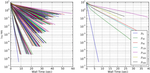
8/3), over time spanT = 40.96 . . . 65 4-9 Comparison of convergence rates for parallel multigrid versus parallel

MINRES, and parallel conjugate gradient implementations for solving discrete LSS equations for Lorenz System, perturbations toρ, (ρ= 28,

σ = 10,β = 8/3), (α= 10√10, T = 81.96, ∆t= 0.01), np = 2 . . . . 67 4-10 Solutions to the LSS equations, the Lagrange multipliers w(t), and

the tangent solution v(t), colored by the local time-dilationη(t) . . . 68 4-11 Iso-surfaces of the Q-Criterion for an example flow field produced by

HIT, (Q= 1_{2 k}Ω_k2 f − kSk2f , Ω = 1_{2 ∇}U _{− ∇}UT ,S= 1_{2 ∇}U +_∇UT ) . . . 70 4-12 Q-Criterion iso-surfaces for several primal solutions (Reλ = 33.06) . . 75 4-13 Average cumulative energy spectrum ¯E, for primal solution to HIT . 76 4-14 LSS vs. Finite Difference sensitivity estimates. Finite differences

com-puted using two primal solutions with the forcing magnitude altered by_±5% (∆β =_±0.05). LSS estimate computed using parallel multi-grid and equation (3.15). . . 78 4-15 Absolute value of instantaneous spectrum sensitivity for various wave

number magnitudes (|k|2) computed from LSS. Dashed lines illustrate

this instantaneous sensitivity measure at several values of _|k_|2. Solid

lines show a few examples curves where the wave number magnitudes are explicitly labeled. . . 79 4-16 Q-Criterion of Lagrange multiplier field (w) at several points in time . 80

List of Tables

4.1 Example Paths taken in Figure 4-3 . . . 55 4.2 Climate Sensitivity values of Lorenz System at (ρ = 28, σ = 10, β =

8/3, z0 = 0). LSS parameters (α = 10

√

10, T = 81.96, ∆t = 0.01). Equations solved to a relative tolerance of 10−8 _{. . . . 67}

Chapter 1

Introduction

1.1

Motivation

Sensitivity analysis is an important tool for engineering design. It deals with finding the sensitivity of the outputs of a system, due to arbitrary perturbations to system parameters. Gradient based optimization techniques rely on sensitivity information to find optimal design specifications for complex engineering systems. Therefore, accurately and cheaply computing this sensitivity can make a large impact on the ability of engineers to effectively explore a particular design space. Adjoint and forward sensitivity approaches can be used to efficiently compute the sensitivity of a system with respect to perturbations in the equations that govern that system. However, while these methods have been very successful in the realm of steady state problems, there has been some difficulties in applying the methods toward time-dependent, or dynamical, systems.

The long-time-averaged properties of a dynamical system are of particular interest when dealing with unsteady systems. In the field of climate science, for example,

there is a substantial need to predict the effects of climate forcing from humans or otherwise. Likewise, in the Aerospace field, the issue of understanding, and designing in situations where unsteady, turbulent fluid flow occurs is of great importance. There are many problems where current turbulence models fail, and only direct simulation of the flow field can model all of the complex dynamics that occur. In these situations scientists and engineers are often most interested in the “climate”, that is, the averaged properties of the system, rather than information and one particular instance in time.

However, analyzing the “climate” of a dynamical system, presents many difficul-ties even for simple chaotic maps and ordinary differential equations (ODE). The problem worsens for the chaotic partial differential equations (PDE) that appear in turbulent fluid flow problems. These problems even persist in comparatively sim-ple periodic systems.Climate sensitivity analysis, which is critical for understanding these systems, has remained computationally out of reach for all but the most simple problems. Only simple finite difference methods have been effective at estimating sensitivities for general chaotic systems. Computation of sensitivities with these methods is inefficient and the computational effort scales poorly with the problem size, parameter space, and time scale needed. The more advanced adjoint and tan-gent sensitivity methods have been difficult to adapt to finding long-time averaged quantities for ergodic dynamical systems [9, 14, 15, 20]. A recent technique, Least Squares Sensitivity (LSS) has proposed a method for accurately computing the cli-mate sensitivity for chaotic and periodic systems, but the computational feasibility is still an issue.

1.2

Climate Sensitivity Problem

This thesis will tackle the climate sensitivity problem, and methods for computing these sensitivities efficiently. The climate problem starts with some set of differential equations (1.1) the model the dynamics of the system of interest.

du

dt =f(u;β) (1.1)

u_∈RM, β ∈Rp (1.2)

Solutions to this differential equations u exist in some M-dimensional phase space where it orbits throughout time infinitely. This u(t) represent anything from the abstract solution vector of an ODE, to the spatially discretized velocity field in an incompressible Navier-Stokes problem. The system dynamics f, are parameterized by some vector β, that represent all the possible problem specific parameters that can affect the solution u. For example, this may include a set of scalar parameters or an entire field of data that can affect the properties of the system. In the climate problem, the long-time average of some function J is examined.

¯ J(β) = lim T→∞ 1 T Z T 0 J( u(t), β) dt (1.3) If the original governing equations are ergodic then the long time average quantities are independent of any initial condition and are dependent only on the system itself, and the parameters β. The goal is then to find the sensitivity of these long time average quantities, ¯J, with respect to perturbations in the governing differential equations, via β.

dJ¯

This thesis will discuss ways of finding this sensitivity dJ¯

dβ, and computing its value

efficiently for large scale problems.

1.3

Previous Work

There have been many attempts at dealing with the problem of climate sensitivity for dynamical systems and chaos in general. Early work by Edward Lorenz first identified the properties of chaos [16] in a chaotic ODE later named the Lorenz System. The main property of chaotic systems is a sensitivity to initial conditions, in other words, small perturbations in the solution at a given time can result in vastly different solutions at a later time. For this reason, the climate, rather than instantaneous solution information, is a more feasible property to examine in chaotic systems. However, Lorenz quickly noticed the difficulty of computing the climate from system information alone [17].

Lea et. al., [14] quantified the problems of using adjoint sensitivity analysis naively on simple chaotic systems, and later confirmed the issue persists in chaotic ocean simulations [15]. Using a typical adjoint formulation, the adjoint equations are solved backwards in time from some terminal condition. However, in chaotic settings, these adjoint equations are unstable and solutions grow unbounded backwards in time [14]. The longer the integration time, the larger the adjoint solutions would grow. One possible solution to this issue is to limit the integration time, but average many these short-time adjoints together. This ensemble adjoint approach was examined by Lea et a. [15] and Eyink et al. [9] for the Lorenz System. However the ensemble approach requires a large number of ensemble solutions to compute approximate sensitivities [15, 9].

describ-ing the solution space by a probability density [22], and computdescrib-ing sensitivities via density perturbations. However, the difficulty of discretizing the phase-space of so-lutions limits its feasibility. In 2007 Abramov and Majda [1] developed a method using fluctuation-dissipation theory from statistical dynamics to estimate sensitivi-ties for statistical quantisensitivi-ties, and has been shown to be successful for certain classes of chaotic systems [2]. Krakos et. al. [13] have developed a method for periodic climate sensitivity problems. This windowing method has made periodic problems feasible even for large scale systems, but this thesis will propose an alternative with several advantages. Recently, Wang [24], proposed a method for computing sensitivi-ties using a shadow trajectory, and relying on the computation of Lyapunov covariant vectors. This shadow-trajectory based method was refined into the development of Least Squares Sensitivity [23]. The climate sensitivity problem is turned into an optimization problem and ultimately the adjoint and tangent sensitivities come as a result of solving a boundary value problem in time, rather than a terminal or initial value problem. This thesis will also examine methods for efficiently solving the LSS equations for large-scale systems.

Chapter 2

Split Periodic Adjoint

2.1

Introduction

The breakdown of traditional sensitivity occurs even in the most simple of periodic dynamical systems. While the occurrence of true periodic systems is rare, the dif-ficulty in efficiently computing sensitivities for periodic systems can provide some insight into the problem for chaotic systems. This section 2.2 will formulate the adjoint sensitivity problem in a new way by splitting the hypothetical perturbation applied to the system into multiple parts. Then section 2.3 will illustrate how this formulation results in a simple set of equations for computing adjoint sensitivities. Finally section 2.4 will describe a method for computing these periodic sensitivity gradients in a more efficient way than previously attainable.[13]

2.2

Formulation

Again, there is a differential equation, defined by f, for finding solutions u(t) given some parameters β.

du

dt =f(u;β) (2.1)

This defines a periodic system for some range of β’s. Solutions for u(t) approaches some unique periodic limit cycle with a period T =T(β). The objective function of interest is J(u;β), and its long-time average ¯J(β). We assume J does not have an explicit dependence onβ, because the sensitivity due to an explicitβ dependence can be computed separately. The goal is to find the sensitivity of this long-time average to perturbations in the parameters β.

¯ J(β) = lim T→∞ 1 T Z T 0 J( u(t);β ) dt (2.2) δJ¯ δβ = ???

As in traditional sensitivity methods we can define the forward tangent equations governingv and the adjoint equations. In this case there will be two different adjoint solutions, φ and ψ, governed by the homogeneous (2.4) and inhomogeneous (2.5) adjoint equations respectively.

dδu dt − ∂f ∂uδu= ∂f ∂β (2.3) dφ dt + ∂f ∂u T φ= 0 (2.4) dψ dt + ∂f ∂u T ψ = ∂J ∂u (2.5)

Solutions for u(t), δu(t), φ(t), and ψ(t) are all periodic with the same period T. Each of these variables, when run from a random initial condition, should converge to some periodic limit-cycle. However, the two adjoint solutions are not unique. The homogeneous adjoint φ satisfies and additional invariant property.

d dt(φ T_{f) =φ}Tdf dt + dφT dt f =φT∂f ∂uf + −φT∂f ∂u f = 0

SinceφT_{f is constant along a trajectory, we can additionally scaleφso thatφ}T_{f = 1,}

this will simplify computations. Because the adjoint equations are linear, new inho-mogeneous solutions may be created by adding a constant multiple of φto any valid

ψ solution.

All possible perturbations in β result in perturbations of f. In a periodic problem there are two fundamental directions that this perturbation (δf) can span, the tan-gent and stable directions. These special directions will be explained and their use motivated in sections 2.2.1 and 2.2.2 respectively. This will result in a decomposition of the perturbation into

δf =δfstable+αf (2.6)

δfstableperturbations will will cause transient deviations from the original limit-cycle.

αis some scalar forcing magnitude, andαf is some forcing that will always be tangent to the original limit-cycle. This decomposition will result in a way to computeδJ/δβ

No Phase Shift Pure Time Dilation General Perturbation

Figure 2-1: Two Possible Perturbations Made to a Periodic Orbit

from stable perturbations and tangent perturbations separately.

δJ¯ δβ = δJ¯ δβ stable + δJ¯ δβ tangent (2.7)

2.2.1

Tangential Component

To compute the tangent contribution, recognize that perturbations tangent to the 1D attractor do not change the shape of the attractor. If a stationary distribution of points along the attractor is computed, then these tangent perturbations simply shift this distribution around. To compute this density the 1D attractor is parameterized

by its arc length s defined by the 1D ODE below

ds

dt =kfk2 (2.8)

The one-dimensional stationary distribution,ρ(s), is effectively a probability density. It represents the probability that after a long time, a trajectory started from a random initial condition will be in that region of phase-space. The total arc-length of the limit cycle is defined asS _≡s(T), and is the total length of the limit-cycle in phase-space. Assuming ergodicity, the density must fulfill the following equation.

¯_b= 1 T Z T 0 b(s(t))dt = Z S 0 ρ(s)b(s) ds (2.9) In other words, the time average of any quantity, b, along the attractor can be computed by integrating the density times the quantity over the arc-length s. This equivalence allows climate estimates to be computed in the time space, as well as the density space. Using this definition, the density in 1D has a simple form, namely that the density at any point along the attractor is inversely proportional the speed at that point. ρ(s) = 1 T 1 kf(s)_k2 (2.10) Density Perturbations

Under tangential forcing (δf = αf, α 1), the density will be perturbed. This section will derive the form that density perturbation will take. For clarity the

following norms will be assumed to be 2-norms (_{k·k ≡ k·k}2) ρ+δρ = 1 T +δT 1 kf +δfk (2.11) 1 ρ+δρ = (T +δT)kf+δfk (2.12) δ 1 ρ = (T +δT)kf+δfk −Tkfk (2.13) Under tangential forcing δf =αf

δ 1 ρ = (T +δT)(1 +α)_kf_{k −}T_kf_k (2.14) =_kf_k(T +αT +δT +αδT ₋T) (2.15) =_kf_k(αT +δT +o(αδT)) (2.16) =_kf_k(αT +δT) (2.17) =kfkT α+δT T (2.18) To compute δT recognize the following:

Z S 0 ρds= 1 (2.19) Z S 0 1 T 1 kf_kds = 1 (2.20) Z S 0 1 kfkds=T (2.21)

So that T +δT = Z S 0 1 kf +δfkds (2.22) = Z S 0 1 (1 +α)_kf_kds (2.23) ≈ Z S 0 1−α+o(α2₎ kf_k ds (2.24) δT =₋ Z S 0 α kfk ds (2.25)

Then δ1_ρ and δρ can be computed.

δ 1 ρ =_kf(s)_kT α(s) + δT T (2.26) =_kf(s)_kT α(s)₋ Z S 0 α(ξ) kf(ξ)_kTdξ (2.27) = 1 ρ α(s)− Z S 0 ρ(ξ)α(ξ) dξ (2.28) δρ =₋ρ2 δ 1 ρ (2.29) =₋ρ21 ρ α(s)₋ Z S 0 ρ(ξ) α(ξ) dξ (2.30) =ρ Z S 0 ρ(ξ)α(ξ)dξ−α(s) (2.31) =ρ (¯α−α) (2.32)

Tangential Sensitivity

Using (2.9), the objective function J can be computed. As well as perturbationsδJ¯. ¯ J = 1 T Z T 0 J(u(t))dt (2.33) = Z S 0 ρ(s)J(u(s))ds (2.34) δJ¯= Z S 0 (ρ δJ +J δρ)ds (2.35) = Z S 0 ρ∂J ∂uδu+J δρ ds (2.36)

Under tangential forcing the shape of the attractor does not change (δu = 0). There-fore all of the sensitivity comes from the δρ term.

δJ¯tangent=

Z S

0

J(u) δρ ds (2.37)

Additionally becauseδρis proportional to ρ, this integral can be converted back into a time integral. δJtangent = Z S 0 J(u)δρ ds (2.38) = Z S 0 ρ(s) (¯α−α)J(u(s) ) ds (2.39) = 1 T Z T 0 (¯α−α) J( u(t) )dt (2.40) By transforming back into the time domain the problem of having to explicitly compute the arc-length and density can be completely avoided. Equation (2.40) has

an intuitive interpretation. A constant tangential forcing will cause no change in the sensitivity gradient, (¯α−α(t) = 0). An increase in the tangential forcing at a point on the attractor causes a proportional decrease in the local density, and therefore a proportional drop in the objective function.

2.2.2

Stable Component

δfstable is defined as being orthogonal to the unforced adjoint φ, (φTδfstable = 0).

Because φT_{f is constant, δf}

stable will never become collinear with f, and the

de-composition will be well defined. Using this definition, computing δfstable from some

arbitrary δf becomes: δf =δfstable+αf φT_{δf =φ}T_δf stable+α φTf (2.41) =α (2.42) δfstable=δf −αf (2.43)

δJ¯stable can then be computed using the regular equation for adjoint sensitivity.

δJ¯stable=− 1 T Z T 0 ψT_δf stable dt (2.44)

2.3

Sensitivity

Using the two decomposed sensitivities the total sensitivity to some generic pertur-bation δf can be computed.

δJ¯=δJ¯tangent+δJ¯stable (2.45) = 1 T Z T 0 (¯α₋α)J(x)₋ψT_δf stable dt (2.46) = 1 T Z T 0 ¯ α J(x)dt₋ 1 T Z T 0 αJ(x) +ψT_δf stable dt (2.47) = ¯αJ¯₋ 1 T Z T 0 J(x)φT_{δf +ψ}T _(δf −αf) dt (2.48) = ¯αJ₋ 1 T Z T 0 J(x)φT_{δf +ψ}T_δf −ψT_{f φ}T_δf dt (2.49) = J T Z T 0 φT_{δf dt} − _T1 Z T 0 J(x)φT_{δf +ψ}T_δf − ψT_f φT_{δf dt (2.50)} =₋1 T Z T 0 −Jφ¯ T _+J(x)φT _+ψT −(ψT_f)φT δf dt (2.51) =₋1 T Z T 0 J(x)₋J¯₋ψT_f φT _+ψT δf dt (2.52)

This takes the form of the normal adjoint sensitivity equation

δJ¯=₋1

T

Z T

0

ηT_{δf dt (2.53)}

With the adjoint variable

η_≡ J(x)₋J¯₋ψT_f

To see how η evolves in time first look at the coefficient of φ. d dt(f T_{ψ) =f}Tdψ dt + dfT dt ψ (2.55) =fT −∂f_∂x T ψ+ ∂J ∂x + ∂f ∂xf T ψ (2.56) =₋fT∂f ∂x T ψ+fT∂J ∂x +f T∂f ∂x T ψ (2.57) =fT∂J ∂x = ∂J ∂x T f (2.58) d dt J( x(t) ) = ∂J ∂x T dx dt (2.59) = ∂J ∂x T f =fT∂J ∂x (2.60) d dt J−J¯−ψ T f = dJ dt − dJ¯ dt − d dt(ψ T f) (2.61) =fT∂J ∂x −0−f T∂J ∂x (2.62) = 0 (2.63)

The coefficient in front of the unforced adjoint φ is simply a constant along the attractor.

c≡ J−J¯−ψT_f

dη dt = d dt c φ+ψ (2.65) =cdφ dt + dψ dt (2.66) =c −∂f_∂x T φ −∂f_∂x T ψ+∂J ∂x (2.67) =₋ ∂f ∂x T c φ+ψ +∂J ∂x (2.68) =₋∂f ∂x T η+∂J ∂x (2.69)

η is also a solution of the same forced adjoint equations and can be computed using any periodic φ and ψ solutions started from random initial conditions. η is simply a special solution that will satisfy:

fT_η=fT _{J −J}¯_−fT_ψ φ+ψ (2.70) = J−J¯−fT_ψ fT_φ+fT_{ψ (2.71)} =J −J¯−fT_ψ+fT_{ψ (2.72)} =J −J¯ (2.73)

2.3.1

Period Sensitivity

This formulation also provides a method for finding the sensitivity of the period T

using equation (2.25). δT =₋ Z S 0 α kfk ds (2.74) =− Z S 0 φT_δf kf_k ds (2.75) =−T Z S 0 1 T 1 kfk φTδf ds (2.76) =₋T Z S 0 ρ φT_{δf ds (2.77)} =₋ Z T 0 φT_{δf dt (2.78)}

Taking this into the more familiar adjoint form, it can be shown that the specific homogeneous adjoint chosen has a physical interpretation. As seen in equation (2.80), the homogeneous adjoint predicts the sensitivity to the log-period (logT) of the system. δlogT = δT T (2.79) =−1 T Z T 0 φT_{δf dt (2.80)}

2.4

Algorithm

This method forces the arbitrary adjointψ towards the correct adjoint trajectory η. After the adjoints have reached a periodic solution, steps 22-24 should be only very small corrections. The quadrature for computing ¯J and δJ¯should be included in

1: # Solve Primal Problem 2: x0 = random vector

3: for i= 1 _→N do

4: xi = ode step(f, xi₋1, ∆t) # some ode stepping (e.g. crank-nicolson)

5: end for

6: # Compute n and k where:

7: # xtakes roughly n steps to reach a periodic trajectory with a period of k

8: # then choose quadrature weights, wi, such that 9: wi = 0 ifi≤n or i > n+k

10: wi = some chosen weights for the k steps from i = _{n + 1, . . . , n+k_}. (e.g. trapezoidal) 11: 12: J¯=PN i=0wi J(xi) = Pn+k i=n+1wi J(xi) # quadrature to find ¯J 13:

14: # Solve Adjoint Problem 15: φN = random vector 16: ψN = random vector

17: for i=N ₋1_→n+ 1 do

18: φi =backward step f, ∂f_∂x, xi, xi+1, φi+1, ∆t, ∂J_∂x = 0

19: ψi =backward step f, ∂f_∂x, xi, xi+1, ψi+1, ∆t, ∂J_∂x = ∂J_∂x

20: # some backward stepping using same method as ode step 21:

22: φi = φi

φT

if(xi) # Normalize φ

23: ci =J(xi)₋J¯₋ψT

i f(xi) # Compute coefficient, should approach zero

24: ψi =ψi+ciφi # Correct ψ onto correct trajectory 25: end for 26: 27: # Compute Sensitivity 28: δJ = −PN_i=0wi ψ_iTδf(xi) = −Pn_i=+_nk₊₁wi ψ_iTδf(xi) # another quadrature to find δJ 29: 30:

the two loops to avoid storing all of the trajectories. This method provides several advantages to the windowing adjoint method [13]. Firstly this estimate only requires one full period of the primal and adjoint dynamics to compute sensitivities. After spin-up the windowing method requires a weighted integration over several period lengths. The split-perturbation technique, however, does require two simultaneous adjoint simulations, nearly doubling the computational time. This will still beat the windowing methods if the window length is more than two periods long. Also, this additional adjoint simulation also provides important sensitivity information about the period of the system without additional cost. Finally, the resulting adjoint solu-tions that are computed provide a time-accurate view of the sensitivity information. This extra information could be vital, for example, in automatic control situations, where time dependent sensitivities could be used for time dependent control inputs.

2.5

Van der Pol Oscillator

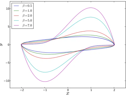
The Van der Pol Oscillator is a second order ODE and one of the simplest systems exhibiting periodic dynamics. This section will examine the application of the pe-riodic adjoint algorithm described in section 2.4. The dynamics of this system are described in equation (2.81) below.

d dt   x y  =   y β(1₋x2_)y−x   (2.81)

Solutions to the differential equation approach a single periodic limit-cycle whose shape is controlled by the parameter β, as is shown in Figure 2-2. The traditional adjoint equations, do not have one unique solution. An example of this phenomenon

2 1 0 1 2

x

y

8 6 4 2 0 2 4 6 8

ψ

_x

ψ

y

J

=x

2

Figure 2-3: Multiple solutions to the adjoint Van der Pol equations, β = 1.0,

J([x, y]) =x2

is shown in figure 2-3. Despite the multiple adjoint solutions there is one “true” adjoint that will predict the correct sensitivities via equation (2.69). The objective function examined here is the averaged squared x position along the attractor. As can be seen in 2-2, a longer and longer proportion of the limit-cycle is further away from the origin as β increases, figure 2-4 confirms this trend.

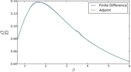
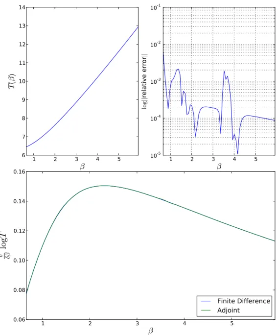
The algorithm from section 2.4 was applied to the Van der Pol system. The adjoint sensitivity estimates are computed for a range of β values. These estimates are compared to a finite difference estimate of the sensitivity. Figure 2-5 shows these sensitivity estimates. Note, that the finite-difference estimates seem to provide worse estimates for a given choice of ∆t, and as ∆t decreases the finite-difference estimates approach the adjoint estimate. Additionally figure 2-6 shows information pertaining the sensitivity of the log-period of the Van der Pol Oscillator. These estimates agree very well with finite-difference estimates.

1 2 3 4 5 6

β

J

(

β

)=

x

Figure 2-4: Objective Function (x2_{) variation versus β}

1 2 3 4 5 6

β

δJ δβ

Finite Difference

Adjoint

Figure 2-5: Predicted sensitivity comparison between split periodic adjoint formula-tion and finite difference (∆t = 10−3_{, ∆β ≈0.16)}

1 2 3 4 5

β

T

(

β

)

β

lo

g

T

Finite Difference

Adjoint

β

re

lat

ive

er

ro

r

Figure 2-6: Predicted period variation (top left), Comparison between predicted sensitivities by FD vs Adjoint (bottom center), and relative error in period sensitivity predictions (∆t = 10−3_{, ∆β ≈0.16) (top right)}

Chapter 3

Least Squares Sensitivity

3.1

Introduction

Least Squares Sensitivity (LSS) is a new technique that can be used to find the sensitivity to long-time average quantities for ergodic dynamical systems. Traditional sensitivity methods derive a initial-value or final-value problem which can then be solved to find sensitivity gradients. However these methods breakdown for the chaotic systems that often occur in engineering settings. The linearized forward-tangent and adjoint equations are unstable and solutions grow unbounded as solutions are solved forward or backward in time. In Least Squares Sensitivity analysis, the problem is instead cast as an optimization problem for finding the smallest perturbation across all time, thus relaxing the initial or terminal condition. The result is a boundary-value problem in time requiring solution for the linearized perturbations across all time simultaneously.

3.2

Formulation of Continuous LSS Equations

To formulate the LSS method we, again, start with a non-linear differential equation for u(t), that represents either an ODE or a spatially discretized PDE of size M

(u_∈RM). We also must obtain some solution to those primal equations u(t). du

dt =f(u) (3.1)

We still want to find a perturbationv(t) that satisfies the linearized equations given some small input perturbation δf

dv dt =

∂f

∂uv+δf (3.2)

However instead of a traditional initial value constraint (i.e. v(t = 0) = 0). We instead require that this perturbation remains small in phase space across time. For computational reasons we also introduce a local time-dilation parameter η(t) that represents the amount of perturbationin time from the primal trajectoryu(t) to its shadow trajectory (u+v). α is a constant describing the relative weighting between minimizing the time-dialation and tangent solution magnitude.

Together these conditions result in the minimization condition

v, η= argmin 1 2 Z T 0 k vk2 2 +α2η2 dt (3.3) s.t. dv dt = ∂f ∂uv+ηf (3.4)

To solve this problem we introduce the Lagrange multiplier w(t) and the Lagrange function Λ Λ = 1 2 Z T 0 vT_{v +α}2_η2 _dt+ Z T 0 wT dv dt − ∂f ∂uv−ηf dt (3.5) δΛ = Z T 0 vT_δv+α2_ηδη+wTdδv dt −w T∂f ∂uδv−f δη dt = Z T 0 δvT v₋ dw dt + ∂f ∂u T w +δη α2η₋wT_f dt + wT_δv T 0 (3.6)

Enforcing the optimality condition that δΛ = 0 for any possible variation (δv, δη) the following equations fall out.

v = dw dt + ∂f ∂u T w (3.7) η = 1 α2f T w (3.8) w(0) =w(T) = 0 (3.9)

Finally, these equations can be manipulated into one second-order linear PDE forw.

−d 2_w dt2 − d dt ∂f ∂u T − ∂f ∂u d dt w+ ∂f ∂u ∂f ∂u T +_P w=δf (3.10) where _Pw= 1 α2f f T_w w(0) = w(T) = 0

The continuous linear operators _B and _E can be defined across time (_Bw)(t)_≡ d dt − ∂f ∂u u(t) w(t) (3.11) (_Ew)(t)_≡1 αf(u(t)) f(u(t)) T_w(t) (3.12) Then Equation (3.10) can be re–written as

BBT ₊ EET

w=δf (3.13)

In this form it is clear that solving for w(t) involves inverting a symmetric positive definite (SPD) linear operator. Finding w(t) directly gives the tangent solution v(t) and time-dilatation η(t) via equations (3.7) and (3.8) respectively. Once v and η

have been found the climate sensitivity can be computed. ¯ J = 1 T Z T 0 J(u(t))dt (3.14) δJ¯= 1 T Z T 0 ∂J ∂uv+ (η−η¯)J dt (3.15)

To actually compute these sensitivities this linear PDE must be discretized and solved.

3.2.1

Discretization of LSS Equations

In order to discretize this problem first the primal solution must first be discretized. Any traditional ODE forward time solving method may be used. This thesis will

assume an implicit trapezoidal method, as a relatively stable and accurate scheme.

un+1−un

∆t =

f(un+1) +f(un)

2 (3.16)

Because of ergodicity, starting from any initial condition (u(0) =u0) will eventually

produce the same long-time average quantities. Since a finite time interval (T) is required an initial condition will be chosen to lie along some attractor. The primal equations can then be solved forward in time to some sufficiently “large” time. From now on u will refer to the vector of all time steps from 0→N. (un≡u(n∆t))

u_≡[u0, u1, u2, . . . uN−1, uN]T, u∈R(N+1)M (3.17)

The linear operators B and E are then discretized at the N midpoints between each time-step. Let’s define

bn _≡ 1 2 ∂f ∂β un +∂f ∂β un+1 ! b_∈RN M _(3.18) fn ≡ 1 2 f(un) +f(un+1) f ∈RN M (3.19) An ≡ ∂f ∂u un+_un+1 2 A∈RN×M×M (3.20)

Then the discretized operators become (Bv)n = vn₋vn+1 ∆t −An vn+vn+1 2 (3.21) (Eη)n = 1 αfnηn (3.22) B ∈RN M×(N+1)M, E ∈RN M×N

B is a bidiagonal block matrix with M _× M blocks. With Fn = I ∆t − An 2 , and Gn =− I ∆t − An

2 . This corresponds to a trapezoidal discretization ofB.

B =         F0 G0 F1 G1 . .. FN₋1 GN−1         E = 1 α         f0 f1 . .. fN₋1        

Using this form BBT _{becomes a block tridiagonal matrix and EE}T _becomes

a block diagonal matrix with rank 1 blocks along the diagonal. The final matrix (S = BBT _+EET_{) retains the SPD form of the continuous linear operator, and}

remains block tri-diagonal with size N M ×N M. This tridiagonal property makes this problem amenable to parallelization, as will be shown in section 4.2.

The final discretized linear equation keeps a form identical to the continuous case as shown below in equation (3.23)

Sw = (BBT +EET)w=b (3.23)

v =−BT_{w (3.24)}

η= 1

αE

Chapter 4

Solution of the Discretized Least

Squares Sensitivity System

4.1

Geometric Multigrid on the LSS System

In order to perform multigrid on the discrete LSS system we must be able to con-struct the system at different coarsening levels and be able to restrict and interpolate solutions between levels. For this problem we use a simple V-cycle, the pseudocode for the algorithm is below.

To fully implement this algorithm we must specify the four functions used above; SMOOTHING, COARSEOPERATOR, RESTRICT, and INTERPOLATE. As well as the recursion conditions and the number of pre and post iterations.

4.1.1

V-Cycle Smoothing Operations

Traditionally in multigrid methods, smoothing iterations are performed using some fixed-point iteration like Jacobi, Gauss-Seidel, SOR, SSOR, etc. The symmetric

1: function VCYCLE(S, b )

2: w0 ←0

3: w1 ← SMOOTHING( S,b, w0, npre )

4: if (Can Coarsen) then

5: r ←b−Sw1 6: rc_← RESTRICT(r ) 7: Sc← COARSEOPERATOR(S ) 8: ec← VCYCLE( Sc, rc) 9: e_← INTERPOLATE(ec ) 10: w2 ←w1+e 11: else 12: w2 ←w1 13: end if 14: w3 ← SMOOTHING( S,b, w2, npost ) 15: return w3 16: end function

tridiagonal block structure of our operator makes something make the block version of these iterations (i.e. block Jacobi, block Gauss-Seidel) possible. For large-scale systems with large M it may be infeasible to actually form the block matrices re-quired to construct a numerical S. Specifically for large PDE systems constructing the Jacobian (∂f_∂u) itself may be difficult. Instead a matrix-free representation for multiplying ∂f_∂u by some vector is used. These fixed iterators require solution of the

M _×M blocks within S repeatedly which can be slow for large M. Additionally, of these methods, only Jacobi iterations can be easily parallelized. A parallelizable Gauss-Siedel/Jacobi hybrid method was tested for this problem. However, because of the SPD features of our matrix more specialized krylov solvers such as Conjugate Gradient and MINRES may be utilized.[3, 6] For the implementation described here standard MINRES iterations were used in all smoothing operations. Using conjugate gradient gave similar convergence characteristics, but MINRES ensured a smoother, monotonic decrease in the solution residual.

Number of Smoothing Iterations

The correct number of pre-smoothing and post-smoothing iterations must be selected to run these smoothing iterations. There unfortunately not much theory on select-ing these parameters optimally. In practice, for LSS problems, a few heuristics for selecting npre and npost have been identified:

• Convergence is largely insensitive to the number of pre-iterations (npre).

• When the number of time-steps is large, a larger number of post-iterations (npost) improves convergence and is often necessary for convergence at all.

• Post-smoothing rapidly reduces the residual at first, but the rate of reduction slows after a few iterations.

• Too much post-smoothing at one level is unproductive and at some point it is better to run a new cycle rather than to continue.

With these rules in mind the number of pre-iterations is chosen to be some small constant number, (e.g. npre = 5). The number of post-iterations was chosen

dynam-ically at runtime. The residual was tracked over many cycles, once the convergence of the residual is below some specified rate the post-smoothing iterator stops. If this minimum rate is chosen correctly this greatly decreases the time it takes for a solution to converge.

4.1.2

Restriction and Interpolation of Solution Residual

For a generic ODE problem all restriction and interpolation are donein time. If the primal problem is a PDE then restriction and interpolation may also be performed

in space. There are potentially two restriction operators Rt and Rx Rt : _RN M

→RNcM (4.1)

Rx : _RN M

→RN Mc (4.2)

Typically in multigrid Nc = N/2 (i.e. restrict to a time-grid of half the size). The same convention will be used here. The scheme for spatial coarsening, however, is completely dependent on the the differential equations used. This issue will be left for section 4.4 when the specific application to a PDE problem is discussed.

When performing time coarsening, a wide windowed average across time-steps i used to coarsen from a time grid of size ∆t to 2∆t. Figure 4-1 shows one way in which the solution on the fine time-grid can restricted to the coarse time-grid.

w0 w1 w2 w3 w4 w5 w6 w7 w8 w9 w10 w11 w12 w13 w14 w15 0 T=N∆t wc 0 w1c w2c w3c w4c w5c w6c w7c 0 T=N 2 2∆t

Figure 4-1: Diagram of Restriction in Time

The restriction operator in this implementation uses a 4 neighbor weighted aver-age on the fine grid to compute the values on the coarse grid. At the internal points

the operator is given by Rt = 1 8         . .. 1 3 3 1 1 3 3 1 . ..        

At the time boundaries t= 0, and T the boundary condition that w(0) =w(T) = 0 must be enforced. The restriction operator must respect this condition when solu-tions are moved from the fine to coarse grid. In the discrete setting ghost points are chosen so that w₋1

2 =w(N−

1 2) = 0.

Using this approach, the equations for the first and last coarsened time-steps are as follows. wc0 = 2 17 3 2w−12 + 3w0+ 3w1+w2 wN/c 2−1 = 2 17 wN−3+ 3wN−2+ 3wN−1+ 3 2wN−1+12

The final time restriction operator Rt is shown in equation (4.3)

Rt =            6 17 6 17 2 17 1 8 3 8 3 8 1 8 . .. 1 8 3 8 3 8 1 8 2 17 6 17 6 17            (4.3)

The interpolation operator, is then simply a constant multiple of the adjoint of the Restriction operator, where the constant is determined so that each of the

non-boundary rows will sum to 1. For this restriction scheme that implies that c= 2.

It=c RT

t (4.4)

4.1.3

LSS Operator Coarsening

The variational form of the coarse grid operator (Sc) is derived from applying the restriction and interpolation operators to the fine-grid matrix (Sc =RSI). However, for large PDE problems, S may not be explicitly computed and therefore neither will Sc. One possible method would be to use a functional form of Sc, in which the operation of the coarse grid operator is computed by the composition of interpolation, application of the fine grid operator, and then restriction. This however would mean each operator application on the coarse grid would be even more expensive than on the fine grid. Because we are using a krylov method as a smoother, almost all the cost of the algorithm is from repeatedly applying the operator to some vector w. This method of forming the coarse grid operator would not take advantage of the fact that solving on the coarser grids should be faster.

To alleviate this problem notice that the fine grid operator is parameterized by some primal trajectory u _∈ R(N+1)M. This primal trajectory, along with the

time-dilation weightingαfully defines the operator. Instead of applying restriction the the whole operator, restriction is applied to the primal trajectory in time and/or space. That coarsened primal solution is then used to define the coarse grid operator.

take every other point in time as shown in (4.5).

u= [u0, u1, u2, . . . uN−1, uN]T

↓ uc _{= [u}

0, u2, u4, . . . uN−2, uN]T (4.5)

However, as uis recursively coarsened in time, the variation from step to time-step grows. Figure 4-2 shows what can happen when the primal is naively coarsened in this fashion. This “jagged” primal will lead to a non-smooth variation in the block matrices along the diagonals of the linear operator. With a non-smooth operator high frequency errors cannot be removed from the solution. The correct coarse grid solution will retain high frequency modes. Instead, when the primal is coarsened it is also smoothed in time. Similar to how the solution residuals are coarsened, a linear operator (Rt,p) can be constructed to restrict the primal solution. This is shown in equation (4.6). This method keeps the end-points of the primal trajectory fixed but smooths the interior points using a weighted average of nearby time-steps. Figure 4-2 shows this compared to the naive method on a primal solution from the Lorenz System. This smoothened primal results in smoother variation across the diagonal of the coarse linear operator. This effectively mimics the important property of the variational coarse operator, namely that solutions on the coarse grid will have smaller

0

1

2

3

4

5

15

5

5

15

x

0

1

2

3

4

5

20

10

0

10

y

0

1

2

3

4

5

t

10

20

30

40

z

Original

Coarsened Naive

Coarsened Smooth

Figure 4-2: Results of coarsening primal four times using naive method (red), and smoothed method (green) (Lorenz Equations)

high-frequency components. Rt,p=               1 1 3 1 1 3 1 . .. 1 3 1 1               (4.6)

For PDE problems the primal trajectory must also be coarsened in space. However, the same spatial restriction operator (Rx) used to spatially coarsen the solution residual may be reused.

4.1.4

Coarsening Order (For PDE’s)

At any given coarsening step there are three options for coarsening. The residual maybe be coarsened in space, time, or both. This choice on the order of coarsening has a profound impact on the convergence of the multigrid scheme. To examine the optimal coarsening strategy a simple sample PDE (Viscous Burger’s Equation (4.7)) will be used. Viscous Burger’s models a simple 1D fluid flow problem, however the equations themselves do no result in chaotic solutions. Instead, the linear LSS system that results from viscous burgers will be used. However, the will be coupled with a primal trajectory from a chaotic system. The primal solution used comes from a 1D slice of a homogeneous isotropic turbulence simulation. The solution of the LSS system for this contrived problem is meaningless, it predicts no relevant sensitivities.

0

1

2

3

4

5

Time Levels

0

1

2

3

Spatial Levels

p

p

p

p

p

p

p

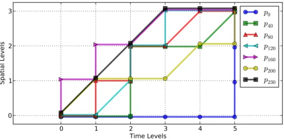
Figure 4-3: Example of space-time coarsening paths (5 Time-Levels × 3 Spatial-Levels)

It only provides a simple test-case for examining different multigrid parameters.

∂u ∂t + 1 2 ∂u2 ∂x =ν ∂2_u ∂x2 (4.7)

The problem of choosing the best coarsening order is one of choosing the optimal path from the finest space-time grid to the coarsest space-time grid. For some chosen problem the solution may be coarsened in time Lt times, and coarsened in space Lx

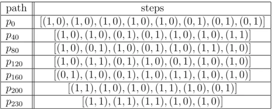
times. At any instance in the cycle the current level is defined as l = (lt, lx). The sequence of forward steps (p) from l = (0, 0) to (Lt, Lx) will define the order in which the coarsening occurs. In this problem a forward step may be one of (1,0), (0,1), or (1,1) which corresponds to time-coarsening, spatial-coarsening, and both respectively. The full V-cycle is then defined by this choice of steps. Figure 4-3 shows several examples of how this path may be selected for Lt = 5, Lx = 3. Table 4.1 shows the steps that make up those paths.

path steps p0 [(1,0),(1,0),(1,0),(1,0),(1,0),(0,1),(0,1),(0,1)] p40 [(1,0),(1,0),(0,1),(0,1),(1,0),(1,0),(1,1)] p80 [(1,0),(0,1),(1,0),(0,1),(1,0),(1,1),(1,0)] p120 [(1,0),(1,1),(0,1),(1,0),(0,1),(1,0),(1,0)] p160 [(0,1),(1,0),(0,1),(1,0),(1,1),(1,0),(1,0)] p200 [(1,1),(1,0),(1,0),(1,1),(1,0),(0,1)] p230 [(1,1),(1,1),(1,1),(1,0),(1,0)]

Table 4.1: Example Paths taken in Figure 4-3

In order to determine the best path a brute force algorithm is used to solve the burger’s LSS system for every possible path from (0,0) to (5,3). For this (Lt, Lx) pair there are 231 unique, single-step, forward paths to try. Figure 4-4 shows the residual of the linear system vs time for all 231 unique paths. The convergence rate varies wildly depending on the coarsening path chosen. For this system, however, the best path is clearly p0. The V-Cycle defined by p0 is one which fully coarsens

in time before coarsening in space. Figure 4-5 shows the 5 paths which provide the fastest rate of convergence. Each of the 5 best paths includes coarsening in time several times before coarsening in space. The ability to further coarsen in time will prove to be very important for the convergence of a multigrid LSS solver.

0 10 20 30 40 50 60 Wall Time (sec)

10-7 10-6 10-5 10-4 10-3 10-2 10-1 100 101 lo g re s 0 5 10 15 20 25 30 35 40

Wall Time (sec) 10-7 10-6 10-5 10-4 10-3 10-2 10-1 100 101 p0 p40 p80 p120 p160 p200 p230

Figure 4-4: Residual v.s. Time For all possible paths, (N = 2048, M = 48)

0

1

2

3

4

5

Time Levels

0

1

2

3

Spatial Levels

4.2

Parallel-In-Time Multigrid

This section will address the techniques used to parallelize the multigrid method described in section 4.1. Specifically, the method for parallelizing this problem along the time axis will be examined. Parallelization along the space axis will be necessary for large classes of PDE’s, however spatial parallelization has been examined in detail elsewhere and maybe added in to this time parallel approach without much difficulty. There are many features of the discrete LSS system derived in section 3.2.1, that can be exploited to more easily parallelize operations on the linear system. Specifi-cally, the block tridiagonal structure greatly reduces the communication complexity. For example, when multiplying by the LSS operator, the result at time-step n only depends on data from time-step n−1 and n+ 1.

To implement the multigrid solver, there are only a few operations that must become parallel. The krylov smoother chosen here, MINRES, requires only the ability to apply some linear operator, to take inner products, and to perform simple arithmetic on vectors, and scalars [18]. The rest of the multigrid algorithm only requires application of the restriction/interpolation linear operators, and application of the primal restriction operator. Once all these operations are parallelized the rest of the multigrid algorithm can run unchanged from the sequential version.

4.2.1

Parallel Distribution of Data

The Lagrange multiplier solution vector, w, for N time-steps, is a size N M vector. The data for this vector will be split across np processes. Assuming that N is a multiple of np, each process will be responsible for Nc = N

np time-steps. The

implementation described here will perform all coarse cycles on the samenpprocesses, this puts a limit on the relationship between the number of time-steps (N), processes

(np), and time-levels (Lt) in the V-cycle.

N =c np 2Lt_{, c∈}

Z+ (4.8)

4.2.2

Parallel Application of the LSS Operator

Application of the LSS linear operator S is the dominant cost of the multigrid cycle. The tridiagonal blocks of theS matrix may not be pre-computed in some PDE cases. In those cases it is more simple to use the decomposition of S from equation (3.23). Making the individual matricesB,BT_{, E, andE}T _{parallel turns out to be an easier}

problem. Multiplying by E, and ET _{is trivial to parallelize in this setting. Each of}

these operators are diagonal, as is their product. (EET_y)

i =fi (fiT yi) (4.9)

The more interesting problem is to parallelize applications of B and BT_{. If the}

original primal trajectory of length N + 1 is split up into Nc+ 1 overlapping sub-chunks as shown in figure 4-6. By forming the B matrix over each sub trajectory, there arenpsub-matrices (Bn). Each sub-matrix transforms an (Nc+1)M vector into nNcM. The sub-matrices can be combined to form the fullB matrix as demonstrated in equation (4.10).

B

=

















B

B

. ..

B

















(4.10)

u

u

u

u

u

u

u

u

u

u

u

u

u

u

u

u

u

n

=0

n

=1

n

=2

n

=3

Figure 4-6: Spiting the primal trajectory into chunks (N = 16, np = 4)

Because the rows of the local operators do not overlap, multiplication by B in parallel simply involves each process multiplying its local (Nc+ 1)M vector by its local sub-matrix. In this step no communication is required.

ApplyingBT _{is the final step towards applying the LSS operator in parallel. More}

care is required to multiply byBT_{. The transpose of the sameBnsub-matrices make}

upBT _{as shown in equation (4.11). If each sub-matrix is multiplied locally the result}

will be mostly identical to multiplication by the global BT_{. However, because the}

rows between matrices overlap the local result is not the whole answer. At each of the overlapping time-steps seen in figure 4-6, the results will be incorrect, and will not match each other. At each of these np₋1 overlapping points the local solution data is summed between neighboring processes. Once this summation is done, each

piece of local data will be correct. BT =                         B₀T B₁T . .. B_nT_p−1                         (4.11)

4.2.3

Parallel Restriction and Interpolation

During restriction and interpolation, the same data splitting described previously is used across all np processes at all Lt time-levels. Because, the parallelization is only over the time domain, spatial restriction and interpolation method may remain unchanged. The time restriction and interpolation operators described in section 4.1.2, are not purely local. That is, in order to restrict the local data on processn, data is required from processn−1 and n+ 1.

Take, for example, anN = 16, time-domain restricted to anN = 8 time-domain, split acrossnp = 4 processes. Process number 1 is responsible for time-steps 4-7 on the fine grid, and 2-3 on the course grid. However, the coarse residual at time-step 2 requires knowledge of the fine-step 3 which is stored on process 0, not locally on process 1. An identical problem occurs when interpolating back from the coarse grid to the fine grid. However, because of the specific restriction operator chosen, only one additional point is required from the neighboring processes to apply the operator. Figure 4-7 shows one example of

r

r

r

r

r

r

r

r

r

r

r

r

r

r

r

r

r

0

r

r

r

r

r

r

r

0

T

n

=1

Figure 4-7: Data dependence for parallel restriction, (N = 16, np = 4)

how this data dependence works out.

Restriction

Each local data chunk is padded with one additional time-step worth of data on each side (Note: the first step of process 0 and the last step of process np −1 are padded with an M-dimensional zero vector) . These additional ghost time-steps are sufficient so that restriction can be done locally. The local time-restriction operators (Rn_t) are 1₂N

np×

N np+ 2

matrices, and are shown in equation (4.12). R_t0=         0 ₁₇6 ₁₇6 ₁₇2 1 8 38 38 18 . .. 1 8 3 8 3 8 1 8         Rn_t =         1 8 38 38 18 1 8 38 38 18 . .. 1 8 38 38 18         0< n < np−1 Rn_tp−1=         1 8 38 38 18 . .. 1 8 38 38 18 2 17 176 176 0         (4.12) Interpolation

The local interpolation operators In

t can be found in a similar way. These size nNp ×

1 2 N np + 2

described before. The local interpolation matrices are shown in equation (4.13) I_t0 = 1 4                0 2 3 1 1 3 . .. 1 3 3 1                Inp−1 t = 1 4            1 3 3 1 . .. 1 3 2 0            I_tn= 1 4            1 3 3 1 . .. 1 3 3 1            0< n < np−1 (4.13) Primal Restriction

The primal restriction operation is the final operator that must be parallelized. The parallel primal trajectory already contains some redundancy, one time-step shared between each pair of processes. However, the specified primal restriction operator requires the primal to be padded similarly to the residual restriction operators. This local primal restriction operators Rn

R0_t,p=         0 1 1 3 1 . .. 1 3 1         Rnp−1 t,p =         1 3 1 1 3 1 . .. 1 3 1         Rn t,p=         1 3 1 . .. 1 3 1 1 0         0< n < np−1 (4.14)

4.2.4

Parallel Arithmetic

The array arithmetic required for parallel MINRES, and other operations required for multigrid are largely trivial. Addition and subtraction can be done locally within each process without any communication. A parallel dot product is simply computed using the sum of all local dot products. Once these operations are parallel there are no other necessary modifications to make the multigrid solver run in parallel.

4.2.5

Implementation Details

The parallel multigrid solver was written in the PythonTM _{programming language.}

Heavy use was made of the NumPy and SciPy projects [12]. The parallelization was developed with MPI using OpenMPI, and specifically the mpi4py Python bindings [8]. The Fast Fourier Transform (FFT) implementation used later in section 4.4, is provided by anfft [7], a NumPy compatible wrapper to the FFTW library [10].

20 15 10 5 0 5 10 15 20

x

0

10

20

30

40

50

z

30 20 10 0 10 20 30

y

0

10

20

30

40

50

z

20

10

0

10

20

x

30

20

10

0

10

20

30

y

Figure 4-8: Example Primal Trajectory for Lorenz System (ρ= 28,σ = 10,β = 8/3), over time span T = 40.96

4.3

ODE Results (Lorenz System)

The Lorenz equations were first formulated by Edward Lorenz as a very low order model of Rayleigh-Bernard Convection [16]. For certain combinations of parame-ters (ρ, σ, β) this third order ODE exhibits chaotic properties. Figure 4-8 shows an example of a solution to the Lorenz equations in the chaotic regime.

d dt      x y z      =      σ(y₋x) x(ρ−z)−y xy₋βz      (4.15) ~u _≡[ x y z ]T

In climate sensitivity problems for the Lorenz attractor, people often examine the time-averaged coordinate positions [14, 19, 20, 24]. Effectively looking at the sensi-tivity of the center of mass of the attractor with respect to changes in the param-eters (ρ, σ, β), another simple perturbation is applying a shift to a coordinate (i.e.

z0 _{= z +z}

0) as shown in (4.16). Perturbations in z0 will then produce an equal

perturbation in the average z coordinate.

d dt      x y z0      =      σ(y−x) x(ρ₋(z0₋z0))−y xy−β(z0−z0)      (4.16)

Unlike for PDE problems, the LSS operatorS, can be fully precomputed for Lorenz system problems. The result is a 3N ×3N sparse matrix with 3×3 blocks. This matrix could be feasibly solved using sparse direct methods, or various krylov solvers. A finely tuned sequential direct solve, could very easily out perform the parallel multigrid implementation described in this thesis. Also, in small ODE problems, like the Lorenz System, com-munication costs required to parallelize these algorithms are non-trivial compared to the overall solution time. Therefore, this section is most useful to verify the parallel multigrid implementation.

4.3.1

Results

The “true” sensitivity to the different parameters in the Lorenz equations have been es-timated in previous works.[14, 24]. These can be used as baselines to verify the parallel LSS solver. Table 4.2 shows various possible objective functions and perturbations, and how the LSS solver compares at computing these sensitivities. In all cases the sensitivity predicted is fairly accurate, in the cases with non-analytical solutions, the estimates lie within previously estimated ranges.

Figure 4-9 shows how the convergence of the multigrid LSS system compares to parallel implementations of conjugate gradient and MINRES on the smae machine. For the cho-sen parameters, the multigrid solver does not dramatically improve on these more simple solvers, however it is slightly better. Figure 4-10 shows the trajectories of the Lagrange multipliers (w) and tangent solution (v) for this problem.

Objective (J) Perturbation Sensitivity LSS Prediction z z0 1 0.9991 x2 z0 0 1.044×10−3 y2 _z 0 0 −9.372×10−3 z ρ 1.01_±0.04 [24] 1.008 x2 _{ρ 2.70±0.10 [24] 2.681} y2 _{ρ 3.87±0.18 [24] 4.027}

Table 4.2: Climate Sensitivity values of Lorenz System at (ρ= 28, σ= 10, β = 8/3,

z0 = 0). LSS parameters (α= 10

√

10, T = 81.96, ∆t = 0.01). Equations solved to a relative tolerance of 10−8

0 2 4 6 8 10 12 14

Wall Time (seconds)

10−9 10−8 10−7 10−6 10−5 10−4 10−3 10−2 10−1 100 101 k b − S w k2 k b k2 Muligrid MINRES Conjugate Gradient

Figure 4-9: Comparison of convergence rates for parallel multigrid versus parallel MINRES, and parallel conjugate gradient implementations for solving discrete LSS equations for Lorenz System, perturbations to ρ, (ρ = 28, σ = 10, β = 8/3), (α = 10√10, T = 81.96, ∆t= 0.01), np = 2

x

1.5

_1.0

0.5 0.0

_0.5

1.0

y

2

1

0

1

2

z

2

1

0

1

2

w

(

t

)

x

0.3 0.2 0.1

0.0 0.1 0.2

_0.3

0.6

0.4

y

0.2

0.0

0.20.4

0.6

z

0.6

0.8

1.0

1.2

1.4

v

(

t

)

Figure 4-10: Solutions to the LSS equations, the Lagrange multipliers w(t), and the tangent solution v(t), colored by the local time-dilationη(t)

4.4

PDE Problem (Homogeneous Isotropic

Tur-bulence)

To validate the LSS solver further, the same solver was run on a model of Homogeneous Isotropic Turbulence (HIT). A traditional HIT solver involves a direct numerical simulation of the three-dimensional Navier-Stokes equations on cube of fluid. The boundaries of the cube are periodic in each direction, and the fluid is forced, deterministically, to drive the flow [11]. Given the correct choice of forcing F, the result is a fully three-dimensional, unsteady, flow, that is chaotic with some bounded energy distribution. Typically, this flow is assumed to be incompressible, as shown in equation (4.17).

∂ ∂tU(x, t) +∇ · U(x, t)⊗U(x, t) =−∇P(x, t) +ν∇2U(x, t) +F( U(x, t) ) (4.17) ∇ ·U(x, t) = 0

The simple, periodic, domain lends itself to a pseudo-spectral solution method. Given a spatial Fourier transform _F, equation (4.19) shows the pseudo-spectral transformation of incompressible Navier-Stokes. ˆG represents the nonlinear convection operator, and is computed in the physical domain (4.20).

ˆ U(k, t) =_F[U(x, t)] (4.18) ∂ ∂tUˆ(k, t) + ˆG ˆ U(k, t)=₋ikPˆ(k, t)₋ν_|k_|2Uˆ(k, t) + ˆFUˆ(k, t) (4.19) k·Uˆ(k, t) = 0

Figure 4-11: Iso-surfaces of the Q-Criterion for an example flow field produced by HIT, (Q= 1₂ kΩk2 f − kSk2f , Ω = 1₂ ∇U− ∇UT , S = 1₂ ∇U+∇UT )