Modelling Exogenous Variability in Cloud Deployments
Giuliano Casale
1Mirco Tribastone
2[email protected]
[email protected]
1
:
Imperial College London, London, United Kingdom
2
:
Ludwig-Maximilians-Universit ¨at, Munich, Germany
ABSTRACT
Describing exogenous variability in the resources used by a cloud application leads to stochastic performance mod-els that are difficult to solve. In this paper, we describe the blendingalgorithm, a novel approximation for queueing net-work models immersed in a random environment. Random environments are Markov chain-based descriptions of time-varying operational conditions that evolve independently of the system state, therefore they are natural descriptors for exogenous variability in a cloud deployment. The algorithm adopts the principle of solving a separate transient-analysis subproblem for each state of the random environment. Each subproblem is then approximated by a system of ordinary differential equations formulated according to a fluid limit theorem, making the approach scalable and computationally inexpensive. A validation study on several hundred models shows that blending can save up to two orders of magnitude of computational time compared to simulation, enabling ef-ficient exploration of a decision space, which is useful in particular at design-time.
1.
INTRODUCTION
Cloud applications run in shared environments where per-formance and availability of computational resources may change over time due to contention from other users. These uncertainties make it difficult to reason at design-time on the performance and availability that an application will of-fer once deployed. Hence, a current research challenge is to identify simple modelling techniques that can effectively account for such variability in performance and availability predictions. In this paper, we propose a methodology for ef-ficient analysis of queueing-based performance models that include a description of exogenous variability, modelled by a continuous-time Markov chain.
Consider, for instance, a decision problem for a multi-tier web application deployed (or to be deployed) on a cloud plat-form. A common performance modelling approach is to rep-resent each software server or virtual machine as a queue and evaluate what-if scenarios by solving the resulting stochas-tic queueing network model using techniques such as ap-proximate mean value analysis [11]. However, upon includ-ing a description of the surroundinclud-ing random environment variability, it is common for the resulting model to become intractable by exact algorithms. Decomposition methods
Copyright is held by author/owner(s).
tackle this problem by assuming a marked separation be-tween the time constants of the system (e.g., the request service times) and those of the random environment (e.g., mean time to failure of a resource) [13]. Under these as-sumptions, one can obtain a solution that is asymptotically exact as the random environment events become increas-ingly less frequent [10]. However, several classes of applica-tions deployed on the cloud donotsatisfy these assumptions. These include, for example, data-intensive applications (e.g., MapReduce) where request service times may last hours and thus resource fluctuations happen repeatedly throughout a request execution period [5]. Similarly, startup times of vir-tual machines may vary from tens of seconds to several min-utes, thus they can introduce significant interference with runtime execution when scaling resources [4].
To cope with the lack of robustness and scalability of exist-ing approximation methods, we introduce theblending algo-rithm, a simple approximation for queueing networks in ran-dom environments. Blending estimates mean performance metrics of the model by evaluating a different transient anal-ysis subproblems for each state of the random environment. Following this principle, the stationary distribution of the original model is obtained as a mixture of the transient be-haviors of each sub-model in isolation. These solutions are related to each other by averaging the initial conditions pro-vided to the transient analysis subproblems, which is a sig-nificant difference compared to simulation as we explain in Section 6. Due to the lack of tractable exact solutions for the transient probability distribution of a queueing network, we use an approximation based on ordinary differential equa-tions (ODEs) in the sense of Kurtz [14]. Crucially, under this formulation the size of the problem does not depend on the number of requests, thus it does not suffer from the state space explosion problem; it only grows with linear complex-ity in the number of stations. Furthermore, the approxima-tion is provably more accurate for increasing job populaapproxima-tion sizes. As a result, blending can analyze problems that are prohibitive to solve with discrete-state models due to the state space explosion problem.
Below we summarize the other major contributions of the present paper, also with respect to an earlier version of the blending algorithm which was proposed in [6] for exponential queueing networks in two-stage random environments:
• We formulate a generalized blending algorithm to study random environments with anarbitrarynumber of states. In the case of a two-stage environment and exponential queues, this algorithm specializes to the one in [6].
0 10 20 30 40 50 −0.1 −0.05 0 0.05 0.1 0.15 experiment number
relative median slowdown
(a) m1.medium 0 10 20 30 40 50 −0.05 0 0.05 0.1 0.15 0.2 experiment number
relative median slowdown
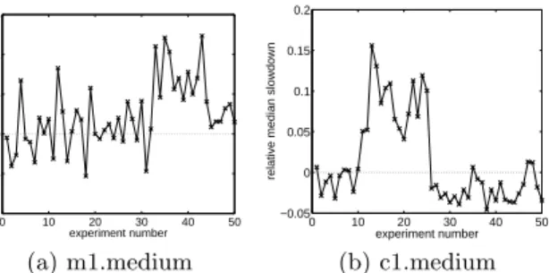
(b) c1.medium Figure 1: Example of exogenous variability in response times for two m1.medium and c1.medium VMs running Apache OFBiz [7]. Each point describes a 10-minutes experiment.
blending algorithm and the exact solution of the model under study.
• We generalize the class of queueing networks supported by the method by allowing Coxian service-time distri-butions, which enable effective approximations of em-pirical service time distributions.
The paper is organized as follows. Section 2 illustrates ogenous variability in a real cloud deployment using an ex-perimental dataset collected on Amazon EC2 and shows lim-itations of decomposition approaches. Our reference model is given in Section 3 and in Section 4, respectively. We define a fluid approximation for the considered queueing models in Section 5 and overview its main properties. This is used in Section 6 to develop the blending algorithm. A numerical validation of the blending algorithm is given in Section 7. Conclusions are given in Section 8.
2.
MOTIVATION
2.1
Random Environment Variability
We discuss the results of an experimental campaign that we have performed on Amazon EC2 Ireland using the demo e-commerce component of Apache OFBiz, an open source enterprise resource planning framework [3]. The aim of the experimental campaign is to illustrate temporal correlation between performance degradations that may be attributed to exogenous factors arising in the cloud deployment envi-ronment. The OFBiz demo application is similar to TPC-W [8] and RUBiS [9], but the framework is more complex since it features several hundreds Java classes and relies on technologies that are common in production systems, such as Groovy dynamic scripting, a template engine, and AJAX on client side.
We have stressed the application using the OFBench suite proposed in [7]. The workload consists of a CPU-bound mix of requests. The OFBiz application is shipped in its basic form with an embedded Geronimo server [2] and an embed-ded Derby in-memory database [1], which we run together inside a single VM. We have deployed OFBiz on several tens ofc1.mediumandm1.mediumVMs on Amazon EC2 Ireland in theeu-west-1aavailability zone. Each VM runs an inde-pendent copy of the application. Simultaneously, we have run the clients, one for each application, inside VMs instan-tiated in the same availability zone. Each experiment uses a single Firefox client coupled with a closed-loop workload
generator. The time between submission of successive re-quests from a client is exponentially distributed with a mean of 1 second. Since there is a single client, we use a short warmup period of 2 minutes. The benchmark discards the sessions executed by the client during the warmup phase of each experiment, since these suffer high response times due to cache misses. After the warmup, the experiment con-tinues at steady-state for 10 minutes before the server is shut down and restarted for the following experiment. Each restart takes approximately 15 minutes to regenerate the database and boot the software. Thus, successive experi-ments inside each VMs are independent. Each experiment is repeated 50 times, for a total of about 15 hours of exper-iments. Notice that we fix in all experiments the random number generator seed to replicate the same sequence of requests, including the client think times, the sequence of request types, and the same random data.
Figure 1 depicts the experimental results. The metric plot is the average response time of the requests experienced by the client, hence it includes also network latency. How-ever, the bandwidth between server and client is normally above 850-900 MBit/sec, as recorded viaiperfat the begin-ning of each experiment, and it does not change significantly throughout the experimental campaign. The metric shown in the figures is defined as follows. We consider the response times of the page with the highest hit rate, i.e., the home-page. Then, we compute the median of its response times across all the experiments and use this a baseline to deter-mine the relative median slowdown within each experiment. The results in the figure show that the deviation from this baseline normally does not exceed 10-15%, but it may last a variable amount of time, from minutes to hours. Since the experiments are independent and the network is largely over-provisioned, it seems reasonable to attribute this slowdown to the VM itself. As a further indication of this, we have studied the same metric for other pages and found nearly identical trends. Notice that our results are quite consistent with the ones reported in [5], which indicate for Amazon EC2 Ireland a CPU variability of approximately 7-8% at 1 hour timescales. However, compared to the study in [5], Figure 1 provides additional information about the tempo-ral correlation of the degradations, suggesting that a state-based model could be useful to describe such perturbations.
2.2
Limitation of Decomposition Approaches
We now show the limitations of decomposition modelling approaches in describing fluctuations in resource capacities such as those illustrated in the previous example. For the sake of illustration, we consider a performance model of a web application represented as a network of queues. This is also the class of models that we focus on in the rest of this paper, even though we expect that the proposed approach is sufficiently general to be extended to other model classes. We consider a queueing network model for a very basic ap-plication deployment involving two VMs running in parallel, havingS1 =S2 = 4 cores each, and a client population of
N = 100 users that issues requests with an average think time of Z = 7s in between successive request arrivals by the same client. A request is randomly sent to any of the two VMs. We assume a two-state random environment that produces fluctuations similar to Figure 1, i.e., for 20% of the time VM2 offers a degraded performance. Service demands of requests are exponentially distributed, operating in the
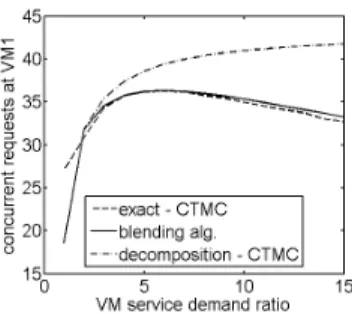
Figure 2: Limitation of classic decomposition approaches. The figure shows in thex-axis the ratio of request service demands at two VMs for a period of degraded performance lasting 20% of the observation time, similarly to Figure 2.
normal regime with the same mean as in the experiments in Figure 1, i.e., 850ms. During the performance degradation, the demand at VM2 increases by a constant factorf. Our what-if analysis consists in studying the system performance as a function of thef degradation factor.
Figure 2 illustrates the predictions. The exact solution is obtained by formulating this model as a continuous-time Markov chain (CTMCs) and solving it directly by numerical methods. The decomposition approach, instead, solves in-dependently of each other the two CTMCs obtained by con-ditioning on the random environment state being the nor-mal regime or the degraded regime. Finally, the blending algorithm anticipates the technique developed in the next section. As we see from the figure, decomposition is unable to correctly characterize this model as the degradation fac-tor increases. This is because the larger the degradation, the more the model will exhibit large and frequent fluctuations of performance metrics over time, which is an event diffi-cult to model by decomposition. Conversely, the method we propose in this paper is more appropriate to evaluate this what-if scenario, besides providing an overall more scalable algorithm than CTMC-based techniques. In the next sec-tions, we provide details about our reference models and introduce formally the blending algorithm, whose computa-tionally properties are finally evaluated in Section 7 against simulation.
3.
MODEL AND NOTATION
In the sequel, we define state the current condition of the queueing network model that represents, e.g., a cloud application, as opposed to the term stage, which instead describes the condition of the random environment, e.g., the cloud deployment or a service offered by the platform.
3.1
Random Environment
The class of random environments considered in this pa-per evolves according to a continuous-time Markov chain, jumping between stages, and specified by the following set of parameters:
• E: number of stages;
• e, h= 1, . . . , E: stage indexes;
• αeh: rate of jump from stageeto stageh;
• αe=Ph6=eαeh: total outgoing rate from stagee;
• peh=αeh/αe: jump probability from stageetoh.
Consider for example the dataset shown in Figure 1. Upon defining a queueing model for the running application, we can assume to describe request service times by the response times obtained in the single-user experiments in Figure 1. The histogram of the mean service times across the experi-ments can be decomposed intoEbins to describe the effect of the random environment on the mean service times. The probability peh is then the probability that a period with
mean service times characterized by bine is followed by a period with mean service times characterized by binh; the mean duration of the periods associated to bin e and h is α−e1, respectively.
3.2
System Model
We denote byM the number of queueing stations and by Nthe number of circulating requests in the model; both val-ues are assumed invariant across stages. All stations have unbounded buffer sizes. Service time processes are indepen-dent and iindepen-dentically distributed random variables following a Coxian distribution, which is a popular parametric model including exponential, hyper-exponential, and Erlang distri-butions as special cases [13]. We shall refer to the states of Coxian service processes asphases.
When the random environment is in stagee, the queueing network is parameterized as follows:
• i, j= 1, . . . , M: station indexes;
• rei,j: routing probability from stationito stationj;
• Sie: number of servers at stationi;
• Kie: number of phases in the Coxian process ati;
• k≡k(i) = 1, . . . , Kie: phase index for stationi;
• µei,k: service rate in phasekat stationi;
• φei,k : probability for requests at i to complete after
service phasek.
We now further specify how stations are affected by ran-dom environment transitions. In our methodology we as-sume that upon stage change, each station state is altered according to a reset rule. That is, for a jump from stage e to h, we define a mapping matrixReh, which is 1 in
el-ement (i, j) if and only theith state in stagee is mapped to the jth state in stageh, 0 otherwise. Note that Reh is
in general rectangular and that multiple states ican jump to the same state j. Also we assume Reh to be such that
there is no loss or generation of mass upon stage transition and that the number of stations and servers does not change with the active stage. Throughout this paper, we illustrate this rule by considering the mapping where the Coxian ser-vice process of the station is restarted upon an environment stage change, meaning that all requests in service are in-stantaneously moved back to phase 1 at that station. Other reset rules are possible, however this has the advantage that the conditional distribution given the current state is always known, but it may overestimate the real service times when the stage jump rate is large.
3.3
Continuous-Time Markov Chain
From the above definitions, the queueing network model may be described by a continuous-time Markov chain (CTMC) having state vector (n, e), wheree= 1, . . . , Eis the current stage of the random environment. The distribution of re-quests across stations is described byn= (n1,n2, . . . ,nM),
ni= (xi, si,1, . . . , si,Ke
i) being the state vector of stationi,
where:1
• si,k is the number of servers that are currently
pro-cessing requests in phase k, thus PKie
k=1si,k =Sie. If
a server is idle, it is counted withinsi,1 together with
the servers processing requests in phase 1. Note that for a delay stationsi,k= +∞.2
• xi = qi+ni,1 is the sum of the number of requests
qi waiting in the queue buffer, and the number of
re-quests ni,1 that are receiving service in phase 1. This
representation provides advantages for the fluid anal-ysis developed in Section 5.
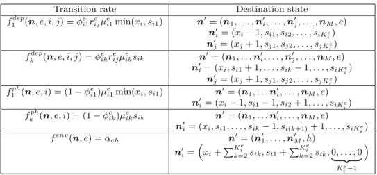
The CTMC defined on the proposed state space may be specified using a collection oftransition rate functionswhich give, for a generic state (n, e), all transition rates at which the process moves to a different state (n0, h). These are given in Table 1. The transitionsf1dep(resp. f
dep
k ) describe
the rates of job completions at stationiat the 1st (resp.kth) Coxian phase that are followed by a departure to stationj; the transitionsf1ph(resp. fkph) describe the rate of requests advancement from the 1st to the 2nd Coxian phase at station i;fenv describe the random environment changing stage.
The infinitesimal generator of the model as a whole may be written as Q= Q1 · · · Q1e · · · Q1E . . . . .. ... . .. ... Qe1 · · · Qe · · · QeE . . . . .. ... . .. ... QE1 · · · QEe · · · QE (1)
where Qe = Q∗e −αeI, Q∗e is the infinitesimal generator
of the queueing network model considered in isolation with stage-e parameterization, I is the identity matrix, and for e6=h,Qeh=αehReh.
Letπ= (π1, . . . ,πe, . . . ,πE) be the vector of equilibrium
probabilities for the model, whereπe refers to stagee. As-suming that the CTMC is ergodic and irreducible, the equi-librium probabilities may be obtained by direct numerical solution of the global balance equationsπQ=0, π1= 1. Unfortunately, due to the combinatorial growth of the state space, direct numerical solutions are prohibitive in most cases of practical interest. This motivates the development of the blending algorithm proposed in this paper.
4.
EMBEDDED PROCESS
To cope with the state space explosion issue, we pro-pose to characterize the equilibrium behavior of the model
1Note that then
istation state vector can be readily mapped
to a canonical state description (ni, ni,1, ni,2, . . . , ni,Ke i),
where ni,k is the number of requests receiving service in
phasekandniis the total number of requests in the queue,
according to the following transformation:
ni=xi+ Kie X k=2 si,k, ni,k= min(xi, si,1), k= 1 si,k, k= 2, . . . , Kei
2In implementations, this value may be set equal to the total
job populationN.
focusing on the network state observed immediately after stage transitions in the random environment. The associ-ated embedded probabilitieshave stationary vector denoted by η = (η1, . . . ,ηe, . . . ,ηE), which represents the
proba-bility distribution embedded at the arrival instant of any random environment event. Thus, each ηe vector, after normalization to sum to unity, may be seen as the entry probability vector in statee at equilibrium. In this section, we first show that theηevectors are related by expressions that describe the transient evolution of the queueing net-work state during the sojourn time within each stage. The blending algorithm, presented in the next sections, leverages on this characterization by approximating the transient evo-lution using Kurtz’s fluid limit theorem and then coupling this method with an outer iterative approximation aimed at approximating the random environment effects. Average steady-state performance indexes are obtained using inter-mediate results of the fluid analysis, as we show in Section 5. The main contribution of this section is the following char-acterization of the embedded probabilitiesηe.
Theorem 1. In the CTMC with generator (1), the em-bedded probabilities satisfy at equilibrium the balance
E X h=1 h6=e phe Z +∞ 0 ηheQ∗htα he−αhtdt Rhe=ηe (2)
for all stagese= 1, . . . , E, wherephe=αhe/αhis the
prob-ability of jump from stage hto stagee. The proof is given in the Appendix.
Theorem 1 enjoys a simple probabilistic interpretation. Let us observe that:
• ηheQ∗htis the transient probability vector at timetfor
the network initialized with probabilityηhin stageh.
• αhe−αht is the exponential density for the time to the
next random environment event.
• ηheQ∗htR
heis the equilibrium entry probability vector
in stageeafter spendingttime units in stageh. Thus, the summation over all source stageshand jump times t in (2), weighted for the jump probabilities peh, simply
provides the stationary entry vectorηe in stagee.
The importance of (2) lies in the fact that, despite not being directly computable due to state-space explosion, the balance relates equilibrium performance metrics, via the vec-tors ηe, with transient analysis, via the integrand ηheQ∗ht
which is a CTMC. This leads us to propose the use of fluid analysis methods, which are effective in transient analysis, for the computation of equilibrium performance metrics in random environments, as we describe next.
5.
FLUID LIMITS
We now leverage on the theory of fluid limits developed by Kurtz [14] to define an approximate transient analysis method for queueing network models. Our intent is to ob-tain an approximation of the integrands of (2) conditional on the random environment being in stageh. Due to this conditioning, in the remainder of this section, we simplify
Transition rate Destination state f1dep(n, e, i, j) =φ e i1rijeµei1min(xi, si1) n0= (n1, . . . ,n0i, . . . ,n0j, . . . ,nM, e) n0i= (xi−1, si1, si2, . . . , siKe i) n0j= (xj+ 1, sj1, sj2, . . . , sjKe i) fkdep(n, e, i, j) =φe ikrijeµeiksik n0= (n1, . . .n0i, . . . ,n 0 j, . . . ,nM, e) n0i= (xi, si1+ 1, . . . , sik−1, . . . , siKe i) n0j= (xj+ 1, sj1, sj2, . . . , sjKe i) f1ph(n, e, i) = (1−φ e i1)µei1min(xi, si1) n0= (n1, . . .n0i, . . . ,nM, e) n0i= (xi−1, si1−1, si2+ 1, . . . , siKe i) fkph(n, e, i) = (1−φeik)µ e iksik n0= (n1, . . .n0i, . . . ,nM, e) n0i= (xi, si1, . . . , sik−1, si(k+1)+ 1, . . . , siKie) fenv(n, e) =αeh n0= (n01, . . . ,n0M, h) n0i= xi+P Ke i k=2sik, si1+ PKie k=2sik,0, . . . ,0 | {z } Ke i−1
Table 1: Transition rate functions. Source state is (n, e) = (n1, . . .ni, . . . ,nM, e).
notation by omitting stage indexes.3 We also consider arbi-trary initial conditions, postponing to Section 6 the defini-tion of the initial condidefini-tions used to approximate (2).
For queueing networks, fluid limits describe the behav-ior of the underlying Markov process as the population of requests N and the number of servers Si at each queue i
grow simultaneously to infinity. Such growth is assumed to be proportional to a scale parameterV that preserves the ratios of servers to requests and which has the interpreta-tion of the system size. Hence, since capacity grows at the same rate of the request population growth, this avoids sat-uration in the asymptotic regime. In the limit regime, the network also maintains the same topology, routing matrix, and service rates of the original model.
Formally, a fluid limit with the above properties is ob-tained by taking a family of CTMCs {YV(t), V ∈ N}
in-dexed by the scale parameter V. Each vector YV(t)
de-scribes the network state at timet according to the state descriptor n, defined as in Section 3, and with transition rates as in Table 1. LetY0be the initial state of the CTMC
at time t = 0. The CTMC Y1(t), where V = 1, is then
the one with states reachable fromY0 through the rates in
Table 1. Similarly,Y2(t), whereV = 2, is the CTMC with
states reachable from the initial state 2Y0through the same
rates. Generalizing, YV(t) is the CTMC with state space
reachable fromVY0, for allV.
The fluid approximation of interest here consists in the limit behavior of thenormalizedCTMCYV(t)/V whenV
grows asymptotically large, with initial stateY0. A
neces-sary condition to apply the limit theorem is that all transi-tion rates enjoy the so-calleddensity-dependentform, which informally states that all CTMC transition rates are propor-tional toV once rewritten in terms of the normalized state descriptorn/V. For instance, making explicit the normal-ized state descriptorn/V in thef1deprates yields
f1dep(n, i, j) =φei1r e ijµ e i1min(Ni, si1) =V φei1r e ijµ e i1min(Ni/V, si1/V) =V f1dep(n/V, i, j). (3) 3
Note that our transient analysis applies also to Coxian queueing networks in the special case of a (non-random) environment with a single stage.
which satisfies the density-dependent form f1dep(n, i, j) =
V f1dep(n/V, i, j) for all stations i, j. Similarly, it can be
shown that all the other transition rates of Table 1 can be expressed in such a form, except the last one that is approximated directly by the blending algorithm without resorting to fluid approximations. In Kurtz’s theory, the density-dependent form implies that a sample path of the normalised CTMC takes increasingly small steps, of order O(1/V), at increasingly large rates, of order O(V). In the limit V →+∞, this allows us to relate a sample path to a continuous trajectory, solution of a system of ordinary dif-ferential equations defined in terms of the density-dependent transition rates of the CTMC, as discussed in the next sub-section.
5.1
Fluid Approximation
Let us first associate ajump vectorto each transition rate function, in such a way to record the component-wise differ-ence between source and destination states in the CTMC. For instance, the jump vector forf1dep(n, e, i, j) is
δdep1 (i, j, e) = (0, . . . ,0,n
0
i−ni,0, . . . ,0,nj0−nj,0, . . . ,0,0)T
and when the stagee is omitted it is similarly defined but with the last element removed. Stemming from the ideas described above, the fluid approximation essentially involves replacing the state descriptor nwith a time-varying deter-ministic vector y(t) and investigating the nonlinear ODE system dy(t) dt = M X i,j=1 Ki X k=1 fkdep(y(t), i, j)δdepk (i, j) + M X i=1 Ki X k=1 fkph(y(t), i)δphk (i) (4) with initial conditionY0. Using Kurtz’s theorem [14,
Theo-rem 3.1] and the fact that the transition rates are Lipschitz continuous everywhere, which implies global existence and uniqueness of the initial value problem (4), it can be shown that, for any finiteT, it holds
lim
V→∞P
supt≤T|YV(t)/V −y(t)| = 0. (5)
asymp-totically undistinguishable in probability, from the unique solution to the ODE system (4). Furthermore, in our model the fluid limit can be shown to implyconvergence in mean[12]:
lim
V→∞E{|YV(t)/V −y(t)|}= 0, t≥0
which provides the motivation for considering the approxi-mationE{YV(t)} ≈Vy(t) that relates the expected queue
length to the re-scaled differential trajectory. This is the in-terpretation herein used and the ODE solution will thus be compared against mean performance indices of the queueing network.
5.2
Example
Let us consider a two-station queueing network with N circulating requests, without a random environment. Sta-tion 1 hasS1servers with exponential service times (K1= 1
phase, rateµ1,1), station 2 hasS2servers with a Coxian
dis-tribution (K2 = 2 phases, rates µ2,1 and µ2,2, completion
probabilitiesφ2,1 and φ2,2 = 1). Station 1 has self-routing
probabilityr1,1 = 1−p, for 0 < p <1, whereas the other
routing probabilities arer1,2=p,r2,1= 1,r2,2= 0.
The state descriptor in the CTMC that models this sys-tem is n = (x1, S1,1, x2, S2,1, S2,2), and we set the initial
condition toY0= (N, S1,0, S2,0). As a result of these
as-sumptions, the definitions in Section 3 specialize to: f1dep(n,1,1) = (1−p)µ1,1min(x1, S1,1),
f1dep(n,1,2) =pµ1,1min(x1, S1,1),
f1dep(n,2,1) =φ2,1µ2,1min(x2, S2,1),
f2dep(n,2,1) =µ2,2S2,2,
f1ph(n,2) = (1−φ2,1)µ2,1min(x2, S2,1),
having jump vectors
δdep1 (1,1) = (0,0,0,0,0)T, δdep1 (1,2) = (−1,0,+1,0,0) T , δdep1 (2,1) = (+1,0,−1,0,0)T, δdep2 (2,1) = (+1,0,0,+1,−1) T δph1 (2) = (0,0,−1,−1,+1) T .
To develop the fluid approximation, we define the determin-istic state vector (x1(t), S1,1(t), x2(t), S2,1(t), S2,2(t)) which
replacesnin the above transition rate functions expressions. Then, (4) provides the nonlinear ODE system
dx1(t) dt =−pµ1,1min(x1(t), S1,1(t)) +µ2,2S2,2(t) +φ2,1µ2,1min(x2(t), S2,1(t)); (6) dS1,1(t) dt = 0; (7) dx2(t) dt =−µ2,1min(x2(t), S2,1(t)) +pµ1,1min(x1(t), S1,1(t)); (8) dS2,1(t) dt =−(1−φ2,1)µ2,1min(x2(t), S2,1(t)) +µ2,2S2,2(t); (9) dS2,2(t) dt =−µ2,2S2,2(t) + (1−φ2,1)µ2,1min(x2(t), S2,1(t)) (10) 0 1 2 3 4 5 6 3 4 5 6 7 8 9 10 t
Queue length at station 1
µ1,1 = 1.0 µ1,1 = 0.6 µ1,1 = 0.8 (a) Plot ofY1(t). 0 1 2 3 4 5 6 10 15 20 25 30 t
Queue length at station 1
µ1,1 = 0.8
µ1,1 = 0.6
µ1,1 = 1.0
(b) Plot ofY3(t).
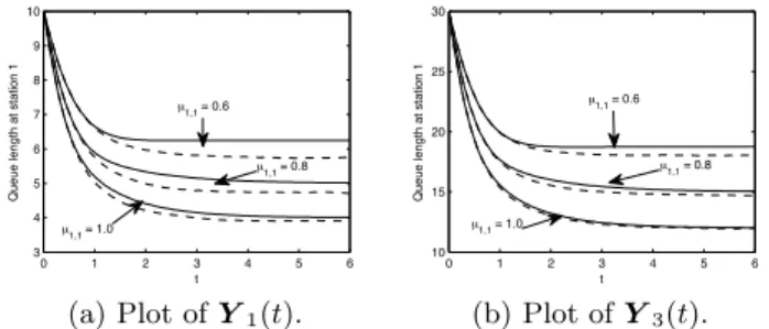
Figure 3: Comparisons between the expected values and the fluid approximation of the queue length at station 1 for the example of Section 5.2 with p = 1.0, φ2,1 = 0,
φ2,2 = 1, µ2,1 = µ2,2 = 2.0, and µ1,1 ∈ {0.6,0.8,1.0}.
Y0 = (10,∞,0,4,0). (a) CTMCY1(t); (b) CTMCY3(t).
Solid lines: ODE solutions; dashed lines: CTMC expected values.
with the initial condition Y0 = (N, S1,0, S2,0), where we
choose arbitrarily to initialize the system with all requests in station 1. The interpretation of the individual ODE terms is similar to the discrete model. For example, (6)–(7) model the state of station 1. Negative fluxes model job departures, while positive fluxes model job arrivals. Null ODEs such as (7) are associated only to stations with exponential servers and indicate that the number of servers available to serve in phase 1 remains constant and, in this example, equal to the initial value S1. Note that the sum of all derivatives (6)–
(10) is zero, which preserves the property of conservation of mass for closed networks.
To numerically illustrate the accuracy of the fluid ap-proximation for transient analysis of queueing networks, let us consider again the example in Section 5.2 and assume the following parameters: p = 1.0, φ2,1 = 0, φ2,2 = 1,
µ2,1 =µ2,2 = 2.0. That is, we consider a tandem network
with no self-routing probabilities where station 2 has Erlang-2 distributed service times with mean 1.0. Three different instances are studied by varying the mean service times at station 1, which is an exponential delay station in this ex-ample since the initial state vector isY0= (10,∞,0,4,0).
Figure 3 shows some representative plots of the CTMC expected values and their fluid approximations during the transient regimes for µ1,1 equal to 0.6, 0.8, and 1.0.
Fig-ure 3(a) plots the queue-length processes at station 1 for the first CTMC,Y1(t), of the family induced by the initial
condition Y0. The ODE solutions (solid lines) are solved
by standard numerical integration whereas the CTMCs were simulated with tight convergence criteria to obtain smooth trajectories for the expectations (dashed lines). The figure shows a generally acceptable quality of the approximation which here tends to increase withµ1,1. The caseµ1,1 = 0.6
has a maximum error of about 8% (at t ≈ 4.0) although the trend of the transient dynamics is still captured well. It is interesting to note that these conditions are quite far away from the many requests/many servers parameteriza-tion considered by the limit theorem, nevertheless the fluid approximation is still usable for transient analysis. This is further backed up by Figure 3(b) which considers the CTMC Y3(t), i.e., a total population of 30 requests and 12 servers
4%, and generally behaves well in all the cases considered. Summarizing, the examples illustrate that fluid limit ap-proximations provide an inexpensive way of evaluating the transient of a queueing network. This feature is at the basis of the blending approximation we introduce in Section 6 for evaluating queueing models with random environments.
5.3
Continuous Mapping
We now turn back to motivating the fluid limit as an ap-proximation for the right-hand side of (2). Let us denote byLh(t) the stochastic process defined by ηheQ∗ht. Each
integral in the inner summation of (2) may be rewritten as Z +∞ 0 Lh(t)αhe −αhtdt. (11) whereLh(t) =ηhe Q∗ht
. Since this does not enjoy a closed-form solution in general, it requires numerical integration over a finite range [0, T], where T is a finite threshold for numerical convergence. Our goal is to show how transient analysis over any range [0, T] may be approximated in terms of the fluid model presented in the previous subsections.
Since the processLh(t) describes the behaviour of the net-work in stagehwhen no stage transitions are possible, it has an asymptotic behaviour according to Section 5.1. There-fore, we may conclude that Lh(t)/V converges in proba-bility, for all 0 ≤ t ≤ T, to yh(t), where V is the scal-ing factor andyh(t) is the fluid model associated with the
network parametrization at the h-th stage of the random environment. We write such a convergence compactly as Lh(t)/V →yh(t). By the continuous mapping theorem [12],
it holds that
Lh(t)αhe−αht/V →yh(t)αhe−αht (12)
for all 0≤t≤T and for anyαh. Thus, the fluid
approxi-mationyh(t) allows us to evaluateV ·yh(t)αhe−αht as an
approximate integrand of (2). This provides the key compu-tational advantage, over the original expression, of requiring only the solution of a small set of ODEs in place of the tran-sient of an intractably large CTMC.
6.
THE BLENDING ALGORITHM
The blending algorithm is an iterative approximation tech-nique that tries to address the state space explosion issue of an exact CTMC analysis. The approach approximates (2) by solving in a cyclic fashion a set ofEODE systems similar to (4). Each ODE system represents the transient behavior of the queueing network model conditional on the random environment being in a given stage. At each cycle, a new set of initial conditions, based on the results at the previous cycle, is provided to theEODE systems. The algorithm is stopped afterCiterations if either a user-specified maximum number of iterations is reached or if the initial conditions as-signed to the ODEs converge to a constant value within a tolerance.
The pseudocode is summarized in Algorithm 1. For each cycle c = 1, . . . , C and stage e = 1, . . . , E, the blending
algorithm solves the ODE system (4) written as dyec(t) dt = M X i,j=1 Ki X k=1 fkdep(y e c(t), i, j)δ dep k (i, j) + M X i=1 Ki X k=1 fkph(yec(t), i)δphk (i). (13) Each trajectoryyec(t) describes the transient behavior of the
queueing network afterttime units since last entering stage e, subject to initial conditionsyec(0),e = 1, . . . , E. At the first iteration, c = 1, yec(0) is initialized similarly to the
example in Section 5.2. That is, the entire job population Nis split in a balanced manner across stations and all server state variables are set tosi,1=Siand tosi,k= 0, for phases
k > 1. At the following iterations the blending algorithm
uses directly (2) to update the initial conditions as yec+1(0) = X h6=e phe Z +∞ 0 kheyhc(t)αhe−αhtRhedt (14)
forc= 2, . . . , C, wherekhe=Pi6=hωiαi,h/
P
j6=eωjαj,eis a
normalizing constant, andωedenotes the equilibrium
prob-ability of stageein the random environment. This normal-izing constant accounts for the fact thatyhc vectors are
prob-ability distributions, whereas the ηhvectors in (2) are not normalized to sum to one. The ratio that defineskheis
sim-ply the ratio of normalizing constants foryec+1(0) andyhc(0),
which only depend on the random environment CTMC and therefore are independent ofc. The algorithm terminates at the first iterationcwhere the maximum improvement over the previous iteration is less than a user-provided conver-gence toleranceδmax(e.g.,δmax= 10−6) or whencexceeds
the maximum number of iterationsC.
Remarks. The blending algorithm differs from techniques such as stochastic simulation in the following sense. In sim-ulation, the system state evolves continuously and the effect of random environment effects is mainly to change the rate of the different events in the simulation and possibly to in-stantaneously change one or more state variables. In order to produce a more efficient evaluation of the model, blend-ing first considers with (13) all the possible sample paths conditional on the model being in stagee. Then, the infor-mation from all these trajectories is averaged in the initial conditions (14) provided in input to the transient subprob-lems at the next iteration. Thus, instead of preserving the state upon stage jump, blending effectively averages all such states into the initial state variable. This allows to simplify the model evaluation at the expense of some approximation error.
6.1
Mean Performance Indexes
The approximate computation of mean performance in-dexes is based on the convergence in mean of Kurtz’s fluid limit. Denote by πe the equilibrium probability of stagee
obtained by solving the random environment CTMC defined by the rates αeh. Let (xe(t)j, sej1(t), sej2(t), . . . , sejKe
j(t)) be
the trajectory of the state of stationjas determined during the final cycle of the blending algorithm. Then the mean queue-length is readily computed as
E[Qj] = E X e=1 πe Z +∞ 0 min(xe(t)j, sej1(t)) + Ke j X k=2 sejk(t) ! dt.
Algorithm 1Blending algorithm pseudo-code
Input:
• model parameters
• : numerical tolerance
• δmax: convergence tolerance
• C >1: maximum number of iterations
Output: approximateye(t),∀e
Algorithm:
Initialize iteration counter: c= 1 Initializeye
c(0) for each stagee= 1, . . . , E.
repeat
c=c+ 1
fore= 1, . . . , Edo
Solve the ODE system (13) foryec+1(t), 0≤t≤T,
with initial valuesyec(0) and tolerance.
end for fore= 1, . . . , Edo Computeyec+1(0) by (14). end for untilmaxe||yec+1(0)−y e c(0)||1< δmaxandc≤C M = 2, E= 2, S= 1 M = 2, E= 2, S= 5 Runtime [s] Runtime [s]
Dist. Error SIM BLE Error SIM BLE
Erl 0.062 806 75 0.062 366 47
Exp 0.078 99 6 0.020 27 6
Cox 0.075 398 11 0.024 204 10
Table 2: Validation results: networks with 2 stations and 2 stages.
The mean throughput is obtained as E[Xj] = E X e=1 πe Z+∞ 0 µej,1min(xe(t)j, sej1(t))φei,1dt.
Both estimates are obtained simply by time-averaging the occupancy measures in the station state vector. In the case of the throughput, these are scaled by the departure rate from stationj. Since in the steady-state the departure rate must be equal in all stages, the throughput in the above expression is given as the departure rate from phase 1.
From these metrics, the mean response time per visit at stationjis readily obtained as
E[Tj] =E[Qj]/E[Xj].
Finally, note that in case of delay servers whereSj = +∞,
the expressions above continue to be finite thanks to our assumption that all servers are initialized in phase 1, thus min(xe(t) j, sej1(t)) =xe(t)j <+∞and alsoP Kej k=2s e jk(t) <
+∞ since the job population is assumed finite and hence the number of active servers never exceedsN.
7.
NUMERICAL VALIDATION
To study the error behavior of blending, we have per-formed an experimental campaign combining a large set of networks with randomly generated configurations, organized
M = 2, E= 10, S= 1 M = 2, E= 10, S= 5
Runtime [s] Runtime [s]
Dist. Error SIM BLE Error SIM BLE
Erl 0.208 6188 15 0.127 5322 18
Exp 0.152 609 4 0.058 166 5
Cox 0.139 1150 19 0.039 1284 23
Table 3: Validation results: networks with 2 stations and 10 stages.
M= 10, E= 2, S= 1 M = 10, E= 2, S= 5
Runtime [s] Runtime [s]
Dist. Error SIM BLE Error SIM BLE
Erl 0.105 64923 17359 0.024 29284 8673
Exp 0.116 5923 1555 0.025 1873 434
Cox 0.158 18238 4127 0.028 14504 1141
Table 4: Validation results: networks with 10 stations and 2 stages.
into groups where a subset of their parameters was kept fixed in order to stress crucial parts of the algorithm.
Overall, we have considered 6 groups of networks with ran-domly generated parameters with different number of queues (M), stages in the random environment (E), and number of servers in each queue (S). The model parameters are drawn from uniform distributions with ranges [0.0,50.0] for the rates of the random environment. The population is equal to N = 50 jobs. Service-time distributions were varied in a controlled form. For each network configuration, we have considered 3 models with an exponential, Erlang-3 (squared coefficient of variationSCV = 1/3), and two-stage Coxian distribution with balanced phase probabilities (SCV = 10), all with the same given means sampled at random from a uniform distribution with range [0.001,10.0]. Varying the service-time distributions allows us to study the impact of a parameter which cannot be captured by an ordinary fluid model of a network without random environment.
For each group we have analyzed 300 models, thus 1800 models were considered overall. Each model was analyzed using Gillespie’s stochastic simulation algorithm. Both sim-ulation and the blending algorithm were implemented in MATLAB, in order to use the same environment to com-pare their runtimes. The implementation of blending al-ternates execution of a non-stiff solver (ode45) and a stiff solver (ode15s) until both methods cannot further improve the (unconditional) mean queue-lengths of the random en-vironment model. We define the minimal improvement in Algorithm 1 to beδmax= 0.01. The maximum number of
iterations is set toC= 100. Furthermore, to speed-up con-vergence, the first iteration of the algorithm terminates by settingye2(0) =y
e
1(0) such that the blending algorithm
per-forms at the first iteration a decomposition approximation computed with the fluid ODEs and initialized with a bal-anced job distribution across queues. This is advantageous particularly for stages with long holding times, since it al-lows the system to immediately accumulate mass on the bot-tleneck station conditional on the current stage. This would be slower using blending since several iterations would be
needed to reallocate the balanced distribution on the bot-tleneck stations.
The results are summarized in Tables 2-4. For each model with a population ofNjobs, the accuracy error is expressed as follows: Error = max 1≤i≤N |QBLE i −QSIMi | N whereQBLEi andQ
SIM
i are the estimates of the steady state
queue length at stationias computed by blending and by simulation, respectively. Each table shows the average errors and execution times for a set of 100 randomly generated net-works, with controlled service time distributions and server multiplicities.
The following observations arise from the results:
• Blending is systematically faster than simulation. In the networks with two stations, the difference in run-times is two order of magnitudes on average, but it tends to decrease with larger network topologies. In the groups of networks with 10 stations (see Table 4), an analysis of the behavior of blending reveals that increased time of the analysis is mainly caused by a larger runtime per single iteration; this is due to the fact that the system of ODEs increases linearly with the number of stations and that larger problems may lead to stiffness for which equations are computation-ally more difficult to solve. The number of iterations, not reported in the table, are found to be quite similar in all groups.
• The accuracy of blending is adequate in all the cases considered, with an expected tendency to decrease with bigger network topologies and more stages of the ran-dom environment.
• By comparing the errors across the same row in every table, we find that increasing the number of servers at each station, while keeping all the other parame-ters the same, leads to an appreciable increase in the quality of the approximation. This is important for practical purposes, since modern multi-core machines often require to consider queues with multiple servers. For such models, we therefore expect our approxima-tion to perform accurately.
• The service-time distributions have an impact on the accuracy error, but this is model-dependent and not easy to interpret. For instance, the cases with Erlang-distributed service times lead to the largest errors in Table 3, whereas they enjoy the smallest errors in the groups of networks of Table 4.
Summarizing, our validation campaign reveals that blend-ing is remarkably faster than simulation, an important prop-erty in particular for optimization-based studies where thou-sands of models need to be evaluated in order to determine a good local optimum. We have performed initial experi-ments in this direction, suggesting that global optimization problems used to solve load-balancing problems that cannot be solved in 2 days using simulation at each iteration of the solver are instead solved in less than 2-3 hours using blend-ing. Approximation errors are acceptable in all cases and importantly they improve sharply as the number of servers in each station increases by a few units, a situation that is typical in applications.
8.
CONCLUSION
Blending is a new technique for the analysis of queue-ing network models in Markov random environments. This class of models can easily find application in describing the performance of cloud software systems, where uncertainties about the deployment environment can be easily modelled in terms of a Markov random environment. A numerical evaluation confirms that the this approach captures trends in performance indexes that these other techniques do not capture.A very attractive feature of our approach is scala-bility, the analysis being based on approximations obtained with ordinary differential equations which are insensitive to the job populations. We have found numerically that the ac-curacy improves with increasing system sizes, which makes our technique particularly appropriate for the analysis of massively parallel systems. Due to the good computational properties, it is readily applicable in decision problems that require the evaluation of the model over large parameter spaces. Several possible extensions of this work may be con-sidered, for instance extensions to multi-class workloads and open models.
Acknowledgement
The work of Giuliano Casale is partially supported by the European project MODAClouds (FP7-318484) and by an EPSRC Small Equipment Funding grant. Mirco Tribastone is supported by the European project ASCENS, 257414.
9.
REFERENCES
[1] Apache Derby project.http://db.apache.org.
[2] Apache Geronimo project.http://geronimo.apache.org. [3] Apache OFBiz project.http://ofbiz.apache.org. [4] M. Mao, M. Humphrey. A Performance Study on the
VM Startup Time in the Cloud. InProc. IEEE Cloud, 423–430, 2012.
[5] J. Schad, J. Dittrich, J.-A. Quian´e-Ruiz. Runtime Measurements in the Cloud: Observing, Analyzing, and Reducing Variance. InProc. of the VLDB Endowment, Vol. 3, No. 1, 2010.
[6] G. Casale, M. Tribastone. Fluid Analysis of Queueing in Two-Stage Random Environments InQEST, pages 21–30. IEEE Computer Society, 2011.
[7] J. Moschetta, G. Casale. OFBench: an Enterprise Application Benchmark for Cloud Resource
Management Studies. InProc. of MICAS workshop -Management of Resources and Services in Cloud and Sky Computing, Sep 2012.
[8] D. F. Garc´ıa and J. Garc´ıa. TPC-W E-commerce benchmark evaluation.Computer, 36(2):42–48, Feb. 2003.
[9] C. Amza, A. Ch, A. L. Cox, S. Elnikety, R. Gil, K. Rajamani, E. Cecchet, and J. Marguerite.
Specification and implementation of dynamic Web site benchmarks. InProc. of IEEE 5th Annual Workshop on Workload Characterization, Oct. 2002.
[10] P. Courtois. Decomposability: Queueing and
Computer System Applications Academic Press, New York, 1977.
[11] D. A. Menasc´e and V. A. F. Almeida.Scaling for E-Business: Technologies, Models, Performance, and Capacity Planning. Prenctice Hall, 2000.
[12] P. Billingsley.Probability and Measure. Wiley, 3rd edition, 1995.
[13] G. Bolch, S. Greiner, H. de Meer, and K. S. Trivedi. Queueing Networks and Markov Chains. 2nd ed., John Wiley and Sons, 2006.
[14] T. G. Kurtz. Solutions of ordinary differential equations as limits of pure Markov processes.J. Appl. Prob., 7(1):49–58, April 1970.
[15] G. Horv´ath, P. Buchholz, and M. Telek. A MAP fitting approach with independent approximation of the inter-arrival time distribution and the lag correlation. InProc. of the 2nd Conf. on Quantitative Evaluation of Systems (QEST), pages 124–133, 2005. [16] M. F. Neuts.Structured Stochastic Matrices of M/G/1
Type and Their Applications. Marcel Dekker, New York, 1989.
APPENDIX
Proof of Theorem 1. From the CTMC generatorQ in
(1), we define two rate matrices
H=diag(Q1, . . . ,Qe, . . . ,QE), M=Q−H,
with the following interpretations.H is a sub-generator in-cluding rates of jumpnotassociated with a random environ-ment transition, whereas the remaining rates are included in matrixM and effectively marked for observation. That is, (H,M) defines a marked point process upon the CTMC generator where arrivals correspond to stage transitions at equilibrium.
Since all transitions are Markovian, the process (H,M) may be seen as an instance of Neuts’s Markovian arrival pro-cess [16], which is a hidden Markov model with phase-type distributed inter-observation times. From basic properties of Markovian arrival processes (e.g., [15, Sec. 2]), the em-bedded distribution at stage transition instants satisfies
η=η(−H)−1M, η1= 1, (15) where (−H)−1M is a stochastic matrix representing the discrete-time Markov chain (DTMC) embedded at stage tran-sition instants.
We now relateηwith the equilibrium distributionπofQ as follows. It is established that the relation between time-stationary distribution and equilibrium distribution of the embedded process is
π=γ−1η(−H)−1, γ=η(−H)−11, (16) where the normalizing constantγ has the probabilistic in-terpretation of mean inter-observation time in the marked process. Exploiting the block diagonal form ofH, we can then simplify (16) as πe=γ −1 ηe(αeI−Q ∗ e) −1 (17) for all stages e = 1, . . . , E. We now make the observa-tion that the matrix inverse in (17) is simply the Laplace transformL(s) of the matrix exponentialeQ∗etevaluated at
s=αe. We can therefore write
πe=γ −1 α−e1 Z +∞ 0 ηeeQ∗etα ee −αet dt (18)
Observe now that, by (16) and (15)
πM=γ−1η(−H)−1M =γ−1η
but this readily implies (2) by rewriting the formula for block e= 1, . . . , Eas
H
X
h=1
πhαheRhe=γ−1ηe