Fitting high-dimensional Copulae to Data

(1)

SFB 649 Discussion Paper 2010-022

Fitting high-dimensional

Copulae to Data

Ostap Okhrin*

* Humboldt-Universität zu Berlin, Germany

This research was supported by the Deutsche

Forschungsgemeinschaft through the SFB 649 "Economic Risk". http://sfb649.wiwi.hu-berlin.de

ISSN 1860-5664

SFB 649, Humboldt-Universität zu Berlin Spandauer Straße 1, D-10178 Berlin

S

FB

6

4

9 E

C

O

N

O

M

I

C

R

I

S

K

B

E

R

L

I

N

(2)

Fitting high-dimensional Copulae to Data

∗

Ostap Okhrin

†

May 13, 2010

Abstract: This paper make an overview of the copula theory from a practical side. We consider

different methods of copula estimation and different Goodness-of-Fit tests for model selection. In the GoF section we apply Kolmogorov-Smirnov and Cramer-von-Mises type tests and calculate power of these tests under different assumptions. Novating in this paper is that all the procedures are done in dimensions higher than two, and in comparison to other papers we consider not only simple Archimedean and Gaussian copulae but also Hierarchical Archimedean Copulae. Afterwards we provide an empirical part to support the theory.

Keywords: copula; multivariate distribution; Archimedean copula; GoF.

JEL Classification: C13, C14, C50.

1 Introduction

Many practical problems arise from modelling high dimensional distributions. Precise modelling is important in fitting of asset returns, insurance payments, overflows from a dam and so on. Often practitioners stay ahead of potential problems by using assets backed up in huge portfolios, payments spatially distributed over land, and dams located on rivers where there are already other hydrological stations. This means that univariate problems are extended to multivariate ones in which all the univariate ones are dependent on each other. Until the late 1990s elliptical distribution, in particular the multivariate normal one, was the most desired distribution in practical applications. However the normal distribution does not, in practice, meet most applications. Some studies (see e.g Fama (1965), Mandelbrot (1965), etc.) show that daily returns are not normally distributed but follow stable distributions. This means that on one hand one cannot take the distribution in which margins are normal, and on the other hand, stable multivariate distributions are difficult to implement. In the hydrological problem, margins arise from extreme value distribution, while one is interested in the maximal value of the water collected after the winter season over a number of years, this value arises from the family

∗_{The ﬁnancial support from the Deutsche Forschungsgemeinschaft via SFB 649 “Okonomisches}

Risiko”, Humboldt-Universit¨at zu Berlin is gratefully acknowledged.

†_{C.A.S.E. - Center for Applied Statistics and Economics, Ladislaus von Bortkiewicz Chair of}

Statistics of Humboldt-Universit¨at zu Berlin, Spandauer Straße 1, D-10178 Berlin, Germany. Email: [email protected]

(3)

● ● ● ● ● ● ● ● ● ● ● ● ● ● ● ● ● ● ● ● ● ● ● ● ● ● ● ● ● ● ● ● ● ● ● ● ● ● ● ● ● ● ● ● ● ● ● ● ● ● ● ● ● ● ● ● ● ● ● ● ● ● ● ● ● ● ● ● ● ● ● ● ● ● ● ● ● ● ● ● ● ● ● ● ● ● ● ● ● ● ● ● ● ● ● ● ● ● ● ● ● ● ● ● ● ● ● ● ● ● ● ● ● ● ● ● ● ● ● ● ● ● ● ● ● ● ● ● ● ● ● ● ● ● ● ● ● ● ● ● ● ● ● ● ● ● ● ● ● ● ● ● ● ● ● ● ● ● ● ● ● ● ● ● ● ● ● ● ● ● ● ● ● ● ● ● ● ● ● ● ●● ● ● ● ● ● ● ● ● ● ● ● ● ● ● ● ● ● ● ● ● ● ● ● ● ● ● ● ● ● ● ● ● ● ● ● ● ● ● ● ● ● ● ● ● ● ● ● ● ● ● ● ● ● ● ● ● ● ● ● ● ● ● ● ● ● ● ● ● ● ● ● ● ● ● ● ● ● ● ● ● ● ● ● ● ● ● ● ● ● ● ● ● ● ● ● ● ● ● ● ● ● ● ● ● ● ● ● ● ● ● ● ● ● ● ● ● ● ● ●● ● ● ● ● ● ● ● ● ● ● ● ● ● ● ● ● ● ● ● ● ● ● ● ● ● ● ● ● ● ● ●● ● ● ● ● ● ● ● ● ● ● ● ● ● ● ● ● ● ● ● ● ● ● ● ● ● ● ● ● ● ● ● ●● ● ● ● ● ● ● ● ● ● ● ● ● ● ● ● ● ● ● ● ● ● ● ● ● ● ● ● ● ● ● ● ● ● ● ● ● ● ● ● ● ● ● ● ● ● ● ● ● ● ● ● ● ● ● ● ● ● ● ● ● ● ● ● ● ● ● ● ● ● ● ● ● ● ● ● ● ● ● ● ● ● ● ● ● ● ● ● ● ● ● ● ● ● ● ● ● ● ● ● ● ● ● ● ● ● ● ● ● ● ● ● ● ● ● ● ● ● ●● ● ● ● ● ● ● ● ● ● ● ● ● ● ● ● ● ● ● ● ● ● ● ● ● ● ● ● ● ● ● ● ● ● ● ● ● ● ● ● ● ● ● ● ● ● ● ● ● ● ● ● ● ● ● ● ● ● ● ● ● ● ● ● ● ● ● ● ● ● ● ● ● ● ● ● ● ● ● ● ● ● ● ● ● ● ● ● ● ● ● ● ● ● ● ● ● ● ● ● ● ● ● ● ● ● ● ● ● ● ● ● ● ● ● ● ● ● ● ● ● ● ● ● ● ● ● ● ● ● ● ● ● ● ● ● ● ● ● ● ● ● ● ● ● ● ● ● ● ● ● ● ● ● ● ● ● ● ● ● ● ● ● ● ● ● ● ● ● ● ● ● ● ● ● ● ● ● ● ● ● ● ● ● ● ● ● ● ● ● ● ● ● ● ● ● ● ● ● ● ● ● ● ● ● ● ● ● ● ● ● ● ● ● ● ● ● ● ● ● ● ● ● ● ● ● ● ● ● ● ● ● ● ● ● ● ● ● ● ● ● ● ● ● ● ● ● ● ● ● ● ● ● ● ● ● ● ● ● ● ● ● ● ● ● ● ● ● ● ● ● ● ● ● ● ● ● ● ● ● ● ● ● ● ● ● ● ● ● ● ● ● ● ● ● ● ● ● ● ● ● ● ● ● ● ● ● ● ● ● ● ● ● ● ● ● ● ● ● ● ● ● ● ● ● ● ● ● ● ● ● ● ● ● ● ● ● ● ● ● ● ● ● ● ● ● ● ● ● ● ● ● ● ● ● ● ● ● ● ● ● ● ● ● ● ● ● ● ● ● ● ● ● ● ● ● ● ● ● ● ● ● ● ● ● ● ● ● ● ● ● ● ● ● ● ● ● ● ● ● ● ● ● ● ● ● ● ● ● ● ● ● ● ● ● ● ● ● ●● ● ● ● ● ● ● ● ● ● ● ● ● ● ● ● ● ● ● ● ● ● ● ● ● ● ● ● ● ● ● ● ●● ● ● ● ● ● ● ● ● ● ● ● ● ● ● ● ● ● ● ● ● ● ● ● ● ● ● ● ● ● ● ● ● ● ● ● ● ● ● ● ● ● ● ● ● ● ● ● ● ● ● ● ● ● ● ● ● ● ● ● ● ● ● −4 −2 0 2 4 −4 −2 0 2 4 ● ● ● ● ● ● ● ● ● ● ● ● ● ● ● ● ● ● ● ● ● ● ● ● ● ● ● ● ●● ● ● ● ● ● ● ● ● ● ● ● ● ● ● ● ● ● ● ● ● ● ● ● ● ● ● ● ● ● ● ● ● ● ● ● ● ● ● ● ● ● ● ● ● ● ● ● ● ● ● ● ● ● ● ● ● ● ● ● ● ● ● ● ● ● ● ● ● ● ● ● ● ● ● ● ● ● ● ●● ● ● ●● ● ● ● ● ● ● ● ● ● ● ● ● ● ● ● ● ● ● ● ● ● ● ● ● ● ● ● ● ● ● ● ● ● ● ● ● ● ● ● ● ● ● ● ● ● ● ● ● ● ● ● ● ● ● ● ● ● ● ● ● ● ● ● ● ● ● ● ● ● ● ● ● ● ● ● ● ● ● ● ● ● ● ● ● ● ● ● ● ● ● ● ● ● ● ● ● ● ● ● ● ● ● ● ● ● ● ● ● ● ● ● ● ● ● ● ● ● ● ● ● ● ● ● ● ● ● ● ● ● ● ● ● ● ● ● ● ● ● ● ● ● ● ● ● ● ● ● ● ● ● ● ● ● ● ● ● ● ● ● ● ● ● ● ● ● ● ● ● ● ● ● ● ● ● ● ● ● ● ● ● ● ● ● ● ● ● ● ● ● ● ● ● ● ● ● ● ● ● ● ● ● ● ● ● ● ● ● ● ● ● ● ● ● ● ● ● ● ● ● ● ● ● ● ● ● ● ● ● ● ● ● ● ● ● ● ● ● ● ● ● ● ● ● ● ● ● ● ● ● ● ● ● ● ● ● ● ● ● ● ● ● ● ● ● ● ● ● ● ● ● ● ●● ● ● ● ● ● ● ● ● ● ● ● ● ● ● ● ● ● ● ● ● ● ● ● ● ● ● ● ● ● ● ● ● ● ● ● ● ● ● ● ● ● ● ● ● ● ● ● ● ● ● ● ● ● ● ● ● ● ● ● ● ● ● ● ● ● ● ● ● ● ● ● ● ● ● ● ● ● ● ● ● ● ● ● ● ● ● ● ● ● ● ● ● ● ● ● ● ● ● ● ● ● ● ● ● ● ● ● ● ● ● ● ● ● ● ● ● ● ● ● ● ● ● ● ● ● ● ● ● ● ● ● ● ● ● ● ● ● ● ● ● ● ● ● ● ● ● ● ● ● ● ● ● ● ● ● ● ● ● ● ● ● ● ● ● ● ● ● ● ● ● ● ● ● ● ● ● ● ● ● ● ● ● ● ● ● ● ● ● ● ● ● ● ● ● ● ● ● ● ● ● ● ● ● ● ● ● ● ● ● ● ● ● ● ● ● ● ● ● ● ● ● ● ● ● ● ● ● ● ● ● ● ● ● ● ● ● ● ● ● ● ● ● ● ● ● ● ● ● ● ● ● ● ● ● ● ● ● ● ● ● ● ● ● ● ● ● ● ● ● ● ● ● ● ● ● ● ● ● ● ● ● ● ● ● ● ● ● ● ● ● ● ● ● ● ● ● ● ● ● ● ● ● ● ● ● ● ● ● ● ● ● ● ● ● ● ● ● ● ● ● ● ● ● ● ● ● ● ● ● ● ● ● ● ● ● ● ● ● ● ● ● ● ● ● ● ● ● ● ● ● ● ● ● ● ● ● ● ● ● ● ● ● ● ● ● ● ● ● ● ● ● ● ● ●● ● ● ● ● ● ● ● ● ● ● ● ● ● ● ● ● ● ● ● ● ● ● ● ● ● ● ● ● ● ● ● ● ● ● ● ● ● ● ● ● ● ● ● ● ● ● ● ● ● ● ● ● ● ● ● ● ● ● ● ● ● ● ● ● ● ● ● ●● ● ● ● ● ● ● ● ● ● ● ● ● ● ● ● ● ● ● ● ● ● ● ● ● ● ● ● ● ● ● ● ● ● ● ● ● ● ● ● ● ● ● ● ● ● ● ● ● ● ● ● ● ● ● ● ● ● ● ● ● ● ● ● ● ● ● ● ● ● ● ● ● ● ● ● ● ● ● ● ● ● ● ● ● ● ● ● ● ● ● ● ● ● ● ● ● ● ● ● ● ● ● ● ● ● ● ● ● ● ● ● ● ● ● ● ● ● ● ● ● ● ● ● ● ● ● ● ● ● ● ● ● ● ● ● ● ● ● ● ● ● ● ● ● ● ● ● ● ● ● ● ● ● ● ● ● ● ● ● ● ● ●● ● ● ● ● ● ● −4 −2 0 2 4 −4 −2 0 2 4 ● ● ● ● ● ● ● ● ● ● ● ● ● ● ● ● ● ● ● ● ● ● ● ● ● ● ● ● ● ● ● ● ● ● ● ● ● ● ● ● ● ● ● ● ● ● ● ● ● ● ● ● ● ● ● ● ● ● ● ● ● ● ● ● ● ● ● ● ● ● ● ● ● ● ● ● ● ● ● ● ● ● ● ● ● ● ● ● ● ● ● ● ● ● ● ● ● ● ● ● ● ● ● ● ● ● ● ● ●● ● ● ● ● ● ● ● ● ● ● ● ● ● ● ● ● ● ● ● ● ● ● ● ● ● ● ● ● ● ● ● ● ● ● ● ● ● ● ● ● ● ● ● ● ● ● ● ● ● ● ● ● ● ● ● ● ● ● ● ● ● ● ● ● ● ● ● ● ● ● ● ● ● ● ● ● ● ● ● ● ● ● ● ● ● ● ● ● ● ● ● ● ● ● ● ● ● ● ● ● ● ● ● ● ● ● ● ● ● ● ●● ● ● ● ● ● ● ● ● ● ● ● ● ● ● ● ● ● ● ● ● ● ● ● ● ● ● ● ● ● ● ● ● ● ● ● ● ● ● ● ● ● ● ● ● ● ● ● ● ● ● ● ● ● ● ● ● ● ● ● ● ● ● ● ● ● ● ● ● ● ● ● ● ● ● ● ● ●● ● ● ● ● ● ● ● ● ● ● ● ● ● ● ●● ● ● ● ● ● ● ● ● ● ● ● ● ● ● ● ● ● ● ● ● ● ● ● ● ● ● ● ● ● ● ● ● ● ● ● ● ● ● ● ● ● ● ● ● ● ● ● ● ● ● ● ● ● ● ● ● ● ● ● ● ● ● ● ● ● ● ● ● ● ● ● ● ● ● ● ● ● ● ● ● ● ● ● ● ● ● ● ● ● ● ● ● ● ● ● ●● ● ● ● ● ● ● ● ● ● ● ● ● ● ● ● ● ● ● ● ● ● ● ● ● ● ● ● ● ● ● ● ● ● ● ● ● ● ● ● ●● ● ● ● ● ● ● ● ● ● ● ● ● ● ● ● ● ● ● ● ● ● ● ● ● ● ● ● ● ● ● ● ● ● ● ● ● ● ● ● ● ● ● ● ● ● ● ● ● ● ● ● ● ● ● ● ● ● ● ● ● ● ● ● ● ● ● ● ● ● ● ● ● ● ● ● ● ● ● ● ● ● ● ●● ● ● ● ● ● ● ● ● ● ● ● ● ● ● ● ● ● ● ● ● ● ● ● ● ● ● ● ● ● ● ● ● ● ● ● ● ● ● ● ● ● ● ● ● ●● ● ● ● ● ● ● ● ● ● ● ● ● ● ● ● ● ● ● ● ● ● ● ● ● ● ● ● ● ● ● ● ● ● ● ● ● ● ● ● ● ● ● ● ● ● ● ● ● ● ● ● ● ● ● ● ● ● ● ● ● ● ● ● ● ● ● ● ● ● ● ● ● ● ● ● ● ● ● ● ● ● ● ● ● ● ● ● ● ● ● ● ● ● ● ● ● ● ● ● ● ● ● ● ● ● ● ● ● ● ● ● ● ● ● ● ● ● ● ● ● ● ● ● ● ● ● ● ● ● ● ● ● ● ● ● ● ● ● ● ● ● ● ● ● ● ● ● ● ● ● ● ● ● ● ● ● ● ● ● ● ● ● ● ● ● ● ● ● ● ● ● ● ● ● ● ● ● ● ● ● ● ● ● ● ● ● ● ● ● ● ● ● ● ● ● ● ● ● ● ● ● ● ● ● ● ● ● ● ● ● ● ● ● ● ● ● ● ● ● ● ● ● ● ● ● ● ● ● ● ● ● ● ● ● ● ● ● ● ● ● ● ● ● ● ● ● ● ● ● ● ● ● ● ● ● ● ● ● ● ● ● ● ● ● ● ● ● ● ● ● ● ● ● ● ● ● ● ● ● ● ● ● ● ● ● ● ● ● ● ● ● ● ● ● ● ● ● ● ● ● ● ● ● ● ● ● ● ● ● ● ● ● ● ● ● ● ● ●● ● ● ● ● ● ● ● ● ● ● ● ● ● ● ● ● ● ● ● ● ● ● ● ● ● ● ● ● ● ● ● ● ● ● ● ● ● ● ● ● ● ● ● ● ● ● ● ● ● ● ● ● ● ●● ● ● ● ● ● ● ● ● ● ● ● ● ● ● ● ● ● ● ● ● ● ● ● ● ● ● ● ● ● ● ● ● ● ● ● ● ● ● ● ● ● ● −4 −2 0 2 4 −4 −2 0 2 4

Figure 1: Scatter plots of bivariate samples with diﬀerent dependency structures

of extreme distributions. As in the previous example, the multivariate extreme value distribution family is also somewhat restrictive.

Two further problems are illustrated in Figure 1. The scatter plot in the first figure shows the realisations of two Gaussian random variables. The points are symmetric and no extreme outliers can be observed. In contrary, the second picture exhibits numerous outliers. The outliers in the first and third quadrants show that extreme values often occur simultaneously for both variables. Such behaviour is observed in crisis periods, when strong negative movements on financial markets occur simultaneously. On the third figure we observe that the dependency between the negative values is different compared to the positive values. This type of non-symmetric dependency cannot be modeled by elliptical distributions, because they impose a very specific radially symmetric dependency structure.

Following these examples we need a solution to easily separate the modelling of the de-pendency structure and the margins. This is one of the tasks of copulae; to enable the modelling of marginals separately from the dependency. The above problem concerning assets could be solved by taking margins from the stable distribution and the dependency, as in the multivariate one. Similar solutions could be found for other problems. In fi-nance, copulae are applied in different fields such as credit portfolio modelling and risk management.

Over the last 40 years, copula has only been attractive from a mathematical perspective, and only as late as 1999 were the different complicated properties of copula, such as the distribution (which made it more flexible), settled and solved. Nowadays dependency plays a key role in many financial models, starting from the basic portfolio theory of

(4)

Markowitz. Recent developments strongly support the joint non-Gaussianity of asset returns and exploit numerous alternative approaches to model the underlying distribution. The key role of dependency can be best illustrated by the famous quote “Given the prices of single-bet financial contracts, what is the price of multiple-bet contracts? There is no unique answer to that question...”. The first application of copulae to financial data was carried out by Embrechts, McNeil and Straumann (1999). In this paper copulae were used in risk management framework which stimulated a series of ground breaking applied papers. Breymann, Dias and Embrechts (2003) model the dependencies of high-frequency data. An application to risk management is discussed in Junker and May (2005). Portfolio selection problems were considered in Hennessy and Lapan (2002) and in Patton (2004). Theoretical foundations of copula-based GARCH models and its application were proposed by Chen and Fan (2005). Lee and Long (2009), Giacomini, Härdle and Spokoiny (2009) and Härdle, Okhrin and Okhrin (2010) consider time varying copulae.

The new fields of application show the need for further theoretical developments. Each proposed model should be estimated with either parametric, semi- or nonparametric meth-ods. The semiparametric estimation of the copula-based distribution, which is based on the nonparametric estimation of margins and estimation of the parameter for the fixed copula function, is discussed in Chen and Fan (2006), Chen, Fan and Tsyrennikov (2006), Genest, Ghoudi and Rivest (1995), Joe (2005), Wang and Wells (2000). Fully nonpara-metric estimation is discussed in Fermanian and Scaillet (2003), Chen and Huang (2007), Lejeune and Sarda (1992). To measure how well a copula-based statistical model fits the data, several goodness-of-fit tests were developed and discussed in the papers by Chen and Fan (2005), Chen, Fan and Patton (2004), Fermanian (2005) and Genest, Quessy and Rémillard (2006), Genest and Rémillard (2008), Breymann et al. (2003). In-depth discussion of simulation methodologies for Archimedean copulae can be found in Whelan (2004) and McNeil (2008). A detailed review and discussion of copula theory is given in Joe (1997) and Nelsen (2006).

In this chapter we describe the attractive features of copulae from the statistical perspec-tive, with examples and applications in real data. We consider the most important copula classes with different methods of estimation and goodness-of-fit tests. We compare differ-ent goodness-of-fit tests by their rejection rates, for which a profound simulation study has been devised. In the empirical part of the chapter we apply different copula models to the normalised residuals and test the quality of the fit by discussed goodness-of-fit tests. We found that for the selected datasets hierarchical Archimedean copula outperform the simple Archimedean copula and the Gaussian copula by all goodness-of-fit tests.

2 Theoretical Background

From the early days of the multivariate probability theory it is well known, that given the

d-variate distribution function F : R → [0; 1] of a d-variate random vector (X1, . . . , Xd)

(5)

X1, . . . , Xd is easily computed:

F1(x) = F(x,+∞, . . . ,+∞),

F2(x) = F(+∞, x,+∞, . . . ,+∞),

· · ·

Fd(x) = F(+∞, . . . ,+∞, x).

The converse problem was studied by Fréchet (1951), Hoeffding (1940), Hoeffding (1941), where having the distribution functions F1, . . . , Fd of d random variables X1, . . . , Xd

de-ﬁned on the same probability space (Ω,F,P) they wanted to make a conclusions about the set Γ(F1. . . , Fd) of thed-variate distribution functions whose marginals areF1, . . . , Fd

F ∈Γ(F1, . . . , Fd)⇔        F1(x) = F(x,+∞, . . . ,+∞), F2(x) = F(+∞, x,+∞, . . . ,+∞), · · · Fd(x) = F(+∞, . . . ,+∞, x).

Nowadays the set Γ(F1, . . . , Fd) is called the Fr´echet class of F1, . . . , Fd. Γ is not empty,

because it always contains the independence case in which F(x1, . . . , xd) = F1(x1)· · · · ·

Fd(xd), ∀x1, . . . , xd ∈ R. Dealing with Fr´echet classes, one often interests in the bounds

and members of the Γ. Dall’Aglio (1972) studies conditions under which there is only one distribution function which belongs to Γ(F1, . . . , Fd). A nice and short review of the

Fr´echet classes can be found in Joe (1997).

In 1959 Sklar found the partial solution to the above mentioned problem by introducing copulae. Because there are a variety of copula definitions we will first look at the most general one. For this we will need to define theC-volume with thed-box that is a cartesian product [a,b] =∏d_j₌₁[aj, bj], where, for every index j ∈ {1,2, . . . , d}, 0≤aj ≤bj ≤1.

Definition 1 For a function C : [0; 1]d _→ _{[0; 1]}_{, the} _C_-volume _V

c of the box [a,b] is defined via Vc([a,b]) def = ∑ v sign(v)C(v),

where the sum is carried over all the 2d vertices v of the box [a,b]. Here also

sing(v) =

{

1, if vj =aj for an even number of vertices,

−1, if vj =aj for an odd number of vertices.

Here is the deﬁnition of a copula, see H¨ardle and Simar (2007):

Definition 2 A function C : [0,1]d →_[0_,_1] _{is a} _d_{-dimensional copula if}

(6)

2. C(1,1, . . . , xj,1. . . ,1) =xj;

3. the Vc-volume of everyd-box[a,b] is positive: Vc([a,b])≥0.

The set of all the d-dimensional copulae (d ≥3) in the rest of the chapter is denoted as Cd, while the set of all bivariate (d = 2) copulae is denoted by C. As already mentioned

above, this simple family of functions has been extremely popular because of its property given in the Sklar (1959) theorem

Theorem 1 Given a d-dimensional distribution function F, a copulaC ∈ Cd exists such

that for all (x1, . . . , xd)∈R

d :

F(x1, . . . , xd) = C{F1(x1), . . . , Fd(xd)}. (1)

The copula C is uniquely defined on ∏d_j₌₁Fj(R) and therefore unique if all margins are

continuous, thus

C(u1, . . . , ud) = F{F1−1(u1), . . . , F_d−1(ud)}. (2)

Conversely, if F1, . . . , Fd are d one-dimensional distribution functions, then the function

F defined in (1) is a d-dimensional distribution function.

Sklar’s theorem also answers the question of the uniqueness of the copula C. However, if, for example, in the two dimensional case at least one of the two distribution functions has a discrete component, there may be more than one copula extendingCfromF1(R)×F2(R)

to the whole unit square [0,1]2. This is due to a fact thatCis uniquely deﬁned only on the product of the rangesF1(R)×F2(R). In this case it is good to have a procedure of bilinear

interpolation in order to single out a unique copula. In the variety of papers where copulae are applied in different fields, authors usually do not consider the assumption that the random variables are continuous. This assumption is necessary to avoid problems with non-uniqueness. The second part of the Sklar’s theorem is based on the construction of the multivariate distribution from the margins and the copula function. It is extremely popular in practice, where, for example, in risk management, analysts may have a better idea about the marginal behaviour of individual risk factors, than about their dependency structure. This approach allows them to combine marginal models and to investigate the sensitivity of risk to the dependence specification.

New multivariate distributions are created in two steps. At ﬁrst, all univariate random variables X1, . . . , Xd are separately described by their marginal distributions F1, . . . , Fd.

Then secondly, the copula C ∈ Cd which contains all the information about the

relation-ship between the original variablesX1, . . . , Xd – not taking into account the information

provided by F1, . . . , Fd – is introduced.

Being armed with the remarks written above, one can write the following copula deﬁnition

Definition 3 Ad-dimensional copula is a cumulative distribution function on [0,1]d_with

(7)

As in the case of the multivariate distribution, mentioned at the beginning, setting all of the arguments equal to +∞ one gets an univariate marginal distribution. A univariate marginal of copula C is obtained by setting some of its arguments equal to 1. Similarly the m-marginal of C,m < d is given by setting all d−m arguments equal to 1, from the simple combinatoric problem, we see that there are (_md)diﬀerent m-margins of the copula

C.

A copulaC satisﬁes a set of diﬀerent important conditions, one of which is the Lipschitz condition which says that:

|C(u1, . . . , ud)−C(v1, . . . , vd)| ≤ d ∑

j=1

|vj −uj|.

Another property says, that ∀j ∈ {1, . . . , d}, {u1, . . . , uj−1, t, uj+1, . . . , ud}, ∀t ∈ [0,1],

the functions t7→C(u1, . . . , uj−1, t, uj+1, . . . , ud) are increasing as functions of t.

To get a better impression of what a copula is from a deﬁnition, let us consider a special bivariate case. Explicitly, a bivariate copula is a functionC : [0,1]2 →[0,1] such that:

1. ∀u∈[0,1] C(u,0) =C(0, u) = 0; 2. ∀u∈[0,1] C(u,1) =C(1, u) =u;

3. ∀u, u′, v, v′ ∈[0,1] withu≤u′ and v ≤v′

C(u′, v′)−C(u′, v)−C(u, v′) +C(u, v)≥0.

The last inequality is referred to as the rectangular inequality and the function that satisﬁes it is said to be 2-increasing. The bivariate copula is always of special interest, because of the properties that are diﬃcult to derive in higher dimensions.

The property of increasingness with respect to each argument could be profound for the bivariate copula in the following way. As we know from above, if C is a bivariate copula, then functions [0,1]∋t7→C(t, v) and [0,1]∋t7→C(v, t) are increasing with respect tot. The increasingness with respect to each argument means that derivatives with respect to Lebegue measure exist almost everywhere, and those derivatives are positive where they exist. From the Lipschitz conditions they are also bound above

0≤ ∂C(s, t)

∂s ≤1, 0≤

∂C(s, t)

∂t ≤1.

Every copula can be expressed in the form of the sum of absolutely continuous and singular part and an absolutely continuous copula C has a density csuch that

C(u1, . . . , ud) = ∫ [0,1]d c(s1, . . . , sd)ds1. . . dsd = 1 ∫ 0 ds1. . . 1 ∫ 0 c(s1, . . . , sd)dsd

from which the copula density is found by diﬀerentiation

c(u1, . . . , ud) =

∂d_C₍_u

1, . . . , ud)

∂u1. . . ∂ud

(8)

Following the Sklar theorem, the multivariate distribution F with margins F1, . . . , Fd

has multivariate density f with marginal densities f1, . . . , fd respectively. If, from the

Sklar theorem copula C exists such that F(x1, . . . , xd) =C{F1(x1), . . . , Fd(xd)} then the

d-variate density is

f(x1, . . . , xd) =c{F1(x1), . . . , Fd(xd)} ·f1(x1). . . fd(xd). (3)

Notice, however, that, as a consequence of the Lipschitz condition, for every bivariate copulaCand for everyv ∈[0,1], both functionst7→C(t, v) andt7→C(v, t) are absolutely continuous so that C(t, v) = t ∫ 0 c1v(s)ds and C(v, t) = t ∫ 0 c2v(s)ds.

Unfortunately, this representation has no application so far.

3 Copula Classes

Naturally, there are an infinite number of different copula functions satisfying the assump-tions of definition. In this section we discuss in details three important classes of simple, elliptical and Archimedean copulae.

3.1 Simple Copulae

Often we are interested in some extreme, special cases, like independence and perfect positive or negative dependence. If d-random variables X1, . . . , Xd are stochastically

in-dependent from the Sklar Theorem the structure of such a relationship is given by the product (independence) copula deﬁned as

Π(u1, . . . , ud) = d ∏

j=1

uj, u1, . . . , ud∈[0,1].

Another two extremes are the lower and upper Fr´echet-Hoeﬀding bounds. They represent the perfect negative and positive dependencies respectively

W(u1, . . . , ud) = max ( 0, d ∑ j=1 uj + 1−d ) , M(u1, . . . , ud) = min(u1, . . . , ud), u1, . . . , ud ∈[0,1].

If, in a two dimensional case C =W and (X1, X2) ∼ C(F1, F2) then X2 is a decreasing

function of X1. Similarly, if C = M, then X2 is an increasing function of X1. In other

words both M and W are singular, where M uniformly spreads the probability mass on the diagonal X1 = X2 and W uniformly spreads the probability mass on the opposite

(9)

x 0.0 0.2 0.4 0.6 0.8 1.0 y 0.0 0.2 0.4 0.6 0.8 1.0 z.lower 0.0 0.2 0.4 0.6 0.8 1.0 x 0.0 0.2 0.4 0.6 0.8 1.0 y 0.0 0.2 0.4 0.6 0.8 1.0 z.prod 0.0 0.2 0.4 0.6 0.8 1.0 x 0.0 0.2 0.4 0.6 0.8 1.0 y 0.0 0.2 0.4 0.6 0.8 1.0 z.upper 0.0 0.2 0.4 0.6 0.8 1.0

Figure 2: Lower Frechet Hoeﬀdings bound, Product copula and upper Frechet Hoeﬀdings bound in two-dimensional case (from left to right).

diagonal X1 = −X2. In general we can argue that an arbitrary copula which represents

some dependency structure lies between these two bounds, i.e.

W(u1, . . . , ud)≤C(u1, . . . , ud)≤M(u1, . . . , ud).

The bounds serve as benchmarks for the evaluation of the dependency magnitude. Note, however, that the lower Fr´echet-Hoeﬀding bound is not a proper copula function ford >2 but is a proper quasi-copula. Both upper and lower bounds are sharp, because there are copulae, that are either equal, at some points, to one of the two bounds.

The simple copulae for the two dimensional case are plotted in Figure 2.

3.2 Elliptical Copulae

Due to the popularity of Gaussian and t-distributions in ﬁnancial applications, elliptical copulae also play an important role. For example, in the modelling of collateralized debt obligations, where the assumption of the Gaussian one-factor dependency between joint default of the obligors, proposed by Li (2000), is seen as a standard approach. The construction of this type of copulae is based directly on the Sklar Theorem. The Gaussian copula and its copula density are given by:

CN(u1, . . . , ud,Σ) =ΦΣ{Φ−1(u1), . . . ,Φ−1(ud)}, cN(u1, . . . , ud,Σ) = =|Σ|−1/2exp { −[Φ−1(u1), . . . ,Φ−1(ud)]′(Σ−1−I)[Φ−1(u1), . . . ,Φ−1(ud)] 2 } , for all u1, . . . , ud∈[0,1],

where ΦΣ is a d-dimensional normal distribution with a zero mean and the correlation

matrixΣ. The variances of the variables are imposed by the marginal distributions. Note, that in the multivariate case the implementation of elliptical copulae is very involved due to technical diﬃculties with multivariate cdf’s. The level plots of the two-dimensional respective densities with diﬀerent margins are given in Figure 3.

(10)

−2 −1 0 1 2 −2 −1 0 1 2 −2 −1 0 1 2 −2 −1 0 1 2

Figure 3: Contour diagrams for Gaussian copula with Gaussian (left column) and t3

distributed (right column) margins.

Using (2) one can derive the copula function for an arbitrary elliptical distribution. The problem is, however, that such copulae depend on the inverse distribution functions and these are rarely available in an explicit form. Therefore, the next class of copulae with its generalisations provides an important ﬂexible and rich family of alternatives to the elliptical copulae.

3.3 Archimedean Copulae

In contrast to elliptical copulae, Archimedean copulae have a special method of construc-tion which does not use (2), but fulﬁlls all the condiconstruc-tions of the copula. Having M as an univariate distribution function of the positive random variable let ϕ be the Laplace transform of M, ϕ =LS(M) ϕ(s) = ∞ ∫ 0 e−swdM(w), s≥0. (4)

Thus,M is said to be the inverse Laplace transform ofϕ,M =LS−1(ϕ). We denote asL the class of Laplace transforms which contain strictly decreasing diﬀerentiable functions, see Joe (1997):

L={ϕ: [0;∞)→[0,1]|ϕ(0) = 1, ϕ(∞) = 0; (−1)jϕ(j) ≥0; j = 1, . . . ,∞}.

It is known, that for an arbitrary univariate distribution functionF, a unique distribution function Gexists such that

F(x) =

∞

∫

0

Gα(x)dM(α) = ϕ{−logG(x)}.

This leads to G= exp{−ϕ[−1]₍_F₎}_{, where}_ϕ[−1] _{is the generalised inverse}

ϕ[−1](x) =

{

ϕ−1(x) for 0≤x < ϕ(0); 0 else.

(11)

Takingd univariate distributions F1, . . . , Fd, a simple extension leads to the multivariate

distribution function that belongs to Γ(F1, . . . , Fd)

F = ∫ Gα₁ . . . Gα_ddM(α) = ϕ(−logG1 − · · · −logGd) = ϕ { _d ∑ j=1 ϕ[−1](Fj) } ,

with Archimedean copula given by

C(u1, . . . , ud) = ϕ { _d ∑ j=1 ϕ[−1](uj) } . (5)

The functionϕis called thegenerator of the Archimedean copula. Throughout the chapter the notationϕ−1 _{is understood as the generalised inverse}_ϕ[−1]_{. Usually generator function}

depends on the parameter θ which is set to be the parameter of the copula. It is easy to see, that Archimedean copulae are exchangeable. In two-dimensional cases they are symmetric in the sense that C(u, v) = C(v, u), ∀u, v ∈ [0,1]. Joe (1997) and Nelsen (2006) provide a classiﬁed list of the typical Archimedean generators. Here we discuss the three most commonly used ones in ﬁnancial applications, Archimedean copulae.

The ﬁrst, widely used (in practice) copula is the Gumbel (1960) copula, which gained its popularity from the extreme value theory. The multivariate distribution based on the Gumbel copula with univariate extreme value marginal distributions is the only extreme value distribution based on an Archimedean copula, see Genest and Rivest (1989). More-over, all distributions based on Archimedean copulae belong to its domain of attraction under common regularity conditions. Direct and inverse generators of the Gumbel copula with the copula function are given by

ϕ(x, θ) = exp{−x1/θ}, 1≤θ <∞, x∈[0,∞), ϕ−1(x, θ) = (−logx)θ, 1≤θ <∞, x∈[0,1], Cθ(u1, . . . , ud) = exp  ₋ { _d ∑ j=1 (−loguj)θ }θ−1 , u1, . . . , ud∈[0,1].

The Gumbel copula leads to asymmetric contour diagrams and shows stronger linkage between positive values, however, is also shows more variability and more mass in the negative tail.

Forθ = 1, the Gumbel copula reduces to the product copula and forθ→ ∞we obtain the Fr´echet-Hoeﬀding upper bound. This copula does not have an extension to the negative dependence. The Gumbel copula is one of a few Archimedean copulae for which we have an explicit form of the distribution function M from (4). In the case of Gumbel copula

M is the stable distribution, see Renyi (1970). This information is very useful in the simulation techniques, especially for the Marshall and Olkin (1988) method, see Section Simulations 4.

Another example is the Clayton (1978) copula which, in contrary to the Gumbel, has more mass on the lower tail, and less on the upper. This copula is often used in the

(12)

modelling of the losses, which is of interest, for example, in insurance and ﬁnance. The necessary functions for this example are

ϕ(x, θ) = (θx+ 1)−1θ, −1/(d−1)≤θ < ∞, θ ̸= 0, x∈[0,∞), ϕ−1(x, θ) = 1 θ(u −θ₋ 1), −1/(d−1)≤θ <∞, θ̸= 0, x∈[0,1], Cθ(u1, . . . , ud) = {( _d ∑ j=1 u−_jθ ) −d+ 1 }−θ−1 , u1, . . . , ud∈[0,1].

The Clayton copula is one of few copulae that has a truncation property and has a simple explicit form of density for any dimension

cθ(u1, . . . , ud) = d ∏ j=1 {1 + (j−1)θ}u−_j(θ+1) ( _d ∑ j=1 u−_jθ−d+ 1 )−(θ−1+d) .

As the parameter θ tends to inﬁnity, dependence becomes maximal and the copula gives the upper Frechet-Hoeﬀding bound. As θ tends to zero, we have independence. As

θ → −1/(d−1), the distribution tends to the lower Fr´echet bound.

Another interesting Archimedean copula is the so called Frank (1979) copula, which, in the bivariate case, is the only elliptical Archimedean copula in the sense that C(u, v) =

u+v−1 +C(1−u,1−v) =C(u, v), where C(u, v) is called the survival or associative copula. C(u, v) is also a copula for a survival bivariate distribution. Direct and inverse generator of the Frank copula with the copula functions are

ϕ(x, θ) = −1 θ log{1 +e u₍_e−θ₋₁₎_}_, ₀_≤_{θ <} _∞_{, x}_∈_[0_,_∞₎_, ϕ−1(x, θ) = log { e−θx₋₁ e−θ−₁ } , 0≤θ <∞, x∈[0,1], Cθ(u1, . . . , ud) = − 1 θ log        1 + d ∏ j=1 {exp(−θuj)−1} {exp(−θ)−1}d−1        , u1, . . . , ud∈[0,1].

The dependence becomes maximal whenθ tends to inﬁnity and independence is achieved when θ = 0.

The level plots of the bivariate copula-based densities with t3 and normal margins are

(13)

0.02 0.04 0.06 0.08 0.1 0.12 0.14 0.16 0.18 0.2 0.22 0.24 −2 −1 0 1 2 −2 −1 0 1 2 0.02 0.04 0.06 0.08 0.1 0.12 0.14 0.16 0.18 0.2 −2 −1 0 1 2 −2 −1 0 1 2 0.02 0.04 0.06 0.08 0.1 0.12 0.14 0.16 0.18 0.2 0.22 0.24 −2 −1 0 1 2 −2 −1 0 1 2 0.02 0.02 0.04 0.06 0.08 0.1 0.12 0.14 0.16 0.18 0.2 −2 −1 0 1 2 −2 −1 0 1 2 0.02 0.04 0.06 0.08 0.1 0.12 0.14 0.16 −2 −1 0 1 2 −2 −1 0 1 2 0.02 0.04 0.06 0.08 0.1 0.12 0.14 −2 −1 0 1 2 −2 −1 0 1 2

Figure 4: Contour diagrams for (from top to bottom) Gumbel, Clayton and Frank copula with Normal (left column) and t3 distributed (right column) margins.

(14)

3.4 Hierarchical Archimedean Copulae

A recently developed ﬂexible method is provided by hierarchical Archimedean copulae (HAC). The special, so called partially nested, case of HAC:

C(u1, . . . , ud) = C0{C1(u1, . . . , uk1), . . . , Cm(ukm−1+1, . . . , ud)} (6) = ϕ0  ∑m p=1 ϕ−₀1◦ϕi    kp ∑ j=kp−1+1 ϕ−_p1(uj)      for ϕ−₀1 ◦ ϕp ∈ {w : [0;∞) → [0;∞)|w(0) = 0; w(∞) = ∞; (−1)j−1w(j) ≥ 0;j =

1, . . . ,∞}, p = 1, . . . , m, with k0 = 1. In contrast to the Archimedean copula, HAC

deﬁnes the whole dependency structure in a recursive way. At the lowest level the depen-dency between the ﬁrst two variables is modelled by a copula function with the generator

ϕ1, i.e. z1 = C(u1, u2) =ϕ1{ϕ1−1(u1) +ϕ−11(u2)}. At the second level an another copula

function is used to model the dependency between z1 and u3, etc. Note, that the

gen-erators ϕi can come from the same family and diﬀer only through the parameter or, to

introduce more flexibility, come from different generator families. As an alternative to the fully nested model, we can consider copula functions, with arbitrarily chosen combinations at each copula level. Okhrin, Okhrin and Schmid (2008) provide several methodologies of determining the structure of the HAC from the data, Okhrin, Okhrin and Schmid (2009) provide necessary theoretical properties of HAC, there are also several empirical papers on the application HAC to CDO (see Choros, Härdle and Okhrin (2009)) and to weather data (see Filler, Odening, Okhrin and Xu (2010)).

4 Simulation Techniques

To investigate the properties of some multivariate distributions, one needs the algorithms of the simulations because many of those properties are to be checked by Monte Carlo techniques. In this section we provide diﬀerent methods of sampling from copula.

4.1 Conditional Inverse Method

The conditional inverse method is a general approach for the simulation of random vari-ables from an arbitrary multivariate distribution. This method can be also used to sim-ulate from copulae. The idea is to generate random variables recursively from the condi-tional distributions. To sample U1, . . . , Ud from copula C we proceed with the following

steps

1. sample V1, . . . , Vd fromU(0,1);

(15)

3. Uj =Cj−1(Vj|U1, . . . , Uj−1) for j = 2, . . . , d where the conditional distribution of Uj is given by Cj(uj|u1, . . . , uj−1) = P(Uj ≤uj|U1 =u1. . . Uj−1 =uj−1) (7) = ∂j−1_C j(u1,...,uj) ∂u1...∂uj−1 ∂j−1_C j−1(u1,...,uj−1) ∂u1...∂uj−1 with Cj =C(u1, . . . , uj,1, . . . ,1) = C(u1, . . . , uj).

The approach is numerically expensive, due to high order derivatives ofC and the calcu-lation of the inverse of the conditional distribution function.

4.2 Marshall and Olkin (1988) Method

To simulate from Archimedean copulae a simpler method was introduced in Marshall and Olkin (1988). The idea of the method is based on the fact that Archimedean copulae are derived from Laplace transforms (4). Following Marshall and Olkin (1988) we proceed with the following three steps procedure:

1. sample U from M =LS−1(ϕ);

2. sample independent (V1, . . . , Vd)∼U[0,1];

3. Uj =ϕ{−ln(Vj)/U} for j = 1, . . . , d.

This method works much faster than the classic conditional inverse technique. The draw-back is that the distribution M can only be determined explicitly for a few generator functions ϕ. For example for Gumbel copula M(θ) = St(1/θ,1,[cos{π/(2θ)}]θ) and for Clayton copula M(θ) = Γ(1/θ,1).

4.3 McNeil (2008) Method

Methods of simulation from the diﬀerent HAC structures were proposed in McNeil (2008); this is an extension of the Marshall and Olkin (1988) method. Below is the algorithm for partially nested copulae (6)

1. sample U from M =LS−1(ϕ0);

2. for i= 1, . . . , m sample

Vkp−1+1, . . . , Vkp fromC[ukp−1+1, . . . , ukp; exp{−U ϕ−

1

0 ◦ϕp(·)}]

using Marshall and Olkin (1988) method where

C[ukp−1+1, . . . , ukp; exp{−U ϕ

−1

0 ◦ϕp(·)}]

is the simple Archimedean copula with the generator function given by exp{−U ϕ−₀1◦ ϕp(·)};

(16)

3. (Ukp−1+1, . . . , Ukp)⊤=ϕ0[−log{(Vkp−1+1, . . . , Vkp)⊤}/U], p= 1, . . . , m.

This method, however also has some drawbacks because the inverse Laplace transform of the composition of the generator function does not always have an explicit form. Never-theless, McNeil (2008) provides a list of combinations, which enable this.

5 Estimation

For a given data-set one needs to find an appropriate model, and to estimate the parameter when the model is fixed. In this section we describe different methods of the estimation of the copula from the data. All methods are similar and are based on the equation (2). Having the sample Xij, i = 1, . . . , n, j = 1, . . . , d one needs to estimate the copula. To

estimate the marginal distributions ˆFj(·), j = 1, . . . , d at least three possible methods are

available. The most simple one is to use the empirical distribution function

ˆ Fj(x) = 1 n+ 1 n ∑ i=1 I{Xij ≤x}.

The change of the fraction before the sum from the classical _n1 to _n₊₁1 is made to bound the empirical distribution from 1; otherwise this causes problems in the maximum likelihood (ML) calculation. The inverse function of ˆFj(x) is then an empirical quantile. Instead

of this simplest empirical estimation one can smooth the distribution function by using a kernel method, see H¨ardle and Linton (1994). Using kernel function κ:R →R, ∫ κ = 1 with the bandwidth h >0 one gets following estimator

˜ Fj(x) = 1 n+ 1 n ∑ i=1 K ( x−Xij h ) ,

with K(x) =∫_−∞x κ(t)dt. Apart from nonparametric methods, there is also a parametric method that is based on the assumption of a parametric form of the marginal distribution

Fj(x,αˆj), where αj is the parameter of the distribution, and ˆαj is its estimator based on

the ML method or method of moments. The last case considers the full knowledge of the true marginal distribution Fj(x), which is rare in practice.

In the same way, there are four possible choices of the copula function. Let us ﬁrst determine general margins ˘Fj(x) that could be one of ˆFj(x), F˜j(x), Fj(x,αˆ) or Fj(x).

The empirical copula is then deﬁned as

b C(u1, . . . , ud) = 1 n n ∑ i=1 d ∏ j=1 I{F˘j(Xij)≤uj}. (8)

LetKj, j = 1, . . . , d be the same symmetric kernel for each direction as in the estimation

of marginal distributions, and let hj, j = 1, . . . , d be the set of bandwidths, then the

kernel based copula estimation considered in Fermanian and Scaillet (2003) is

e C(u1, . . . , ud) = 1 n n ∑ i=1 d ∏ j=1 Kj { uj −F˘j(Xij) hj } . (9)

(17)

In the bivariate case (d = 2) to avoid boundary bias, one uses (Chen and Huang, 2007) local linear kernel to smooth at u∈[0,1]

Kuh= K(x){a2(u, h)−a1(u, h)x} a0(u, h)a2(u, h)−a21(u, h) , with aℓ(u, h) = ∫u/h (u−1)/ht

ℓ_K₍_t₎_{dt, ℓ} _{= 0}_,₁_,_{2 and} _{h >} _{0 (see Lejeune and Sarda (1992),}

Jones (1993)). Let Guh(t) =

∫t

−∞Kuh(x)dxand Tuh=Guh{(u−1)/h}, then an unbiased

kernel based estimator of the bivariate copula is given by

e C(u1, u2) = 1 nGu1h { u1−F˘1(Xi1) h } Gu2h { u2−F˘2(Xi2) h } (10) − (u1Tu2h+u2Tu1h+Tu1hTu2h).

The last situation is the parametric copula C(u, θ), where the copula comes from some ﬁxed family. In this case the parameter of the copula function is estimated using the ML method. From (3) the likelihood function for the case ˘Fj(x) = Fj(x, αj), j = 1, . . . , d is

L(θ, α1, . . . , αd) = n ∏

i=1

f(Xi1, . . . , Xid;α1, . . . , αd, θ)

and the log-likelihood function is given by

ℓ(θ, α1, . . . , αd) = n ∑ i=1 logc{F1(Xi1;α1), . . . , Fd(Xid;αd);θ} + n ∑ i=1 d ∑ j=1 logfj(Xij;αj),

where fj(·) are marginal densities. All parameters {θ, α1, . . . , αd} can be estimated in

one or two steps. For practical applications, however, a two step estimation procedure is more eﬃcient. A one step procedure, also called full maximum likelihood, is carried out by maximising likelihood function simultaneously over all parameters, thus by solving

(∂ℓ/∂α1, . . . , ∂ℓ/∂αd, ∂ℓ/∂θ) = 0,

with respect to (θ, α1, . . . , αd). Following the standard theory on ML estimation estimators

are eﬃcient and asymptotically normal. However, it is often computationally demanding to solve the system simultaneously.

The two step procedure can be done for any kind of marginal distribution ˘Fj(x) ∈

{Fbj(x),Fej(x), Fj(x,αˆ)}. Firstly, we estimate the marginal distribution by using any of

the above methods and secondly, we estimate the copula parameter by the pseudo log-likelihood function ℓp(θ) = n ∑ i=1 logc{F˘1(Xi1), . . . ,F˘d(Xid);θ}.

(18)

The solution is then ˆ

θ = arg max

θ

ℓp(θ).

If the marginal distributions are from parametric families ˘Fj(x) =Fj(x,αˆj), j = 1, . . . , d,

then the method is calledinference for margins. Otherwise, if margins, are nonparametri-cally estimated ˘Fj(x)∈ {Fbj(x),Fej(x)}, j = 1, . . . , d, then the method is calledcanonical

maximum likelihood method.

6 Goodness-of-Fit (GoF) Tests

After the copula is estimated, one needs to test how well the estimated copula describes the sample. Nonparametric copula is certainly the best choice for this, and is usually considered the benchmark in many tests. With the GoF tests one checks whether the underlying copula belongs to any copula family. The test problem could be written as a composite null hypothesis

H0 : C ∈ C0, against H1 : C /∈ C0,

where C0 = {Cθ : θ ∈ Θ} is a known parametric family of copulae. In some cases we

restrict ourselves to the one element family C0 = C0, thus the hypothesis in this case in

the simple one. The test problem is, in general, equivalent to the GoF tests for multivariate distributions. However, since the margins are estimated we cannot apply the standard test procedures directly.

Here we consider several methodologies recently introduced in the literature. We can categorised them into three classes: tests based on the empirical copula, tests based on the Kendall’s process and tests based on Rosenblatt’s transform.

6.1 Tests based on the empirical copula

These tests are based directly on the distance between C and C0. Naturally, as C is

unknown one takes the empirical copula which is fully nonparametric ˆC or ˜C instead. The estimated copula C0, that should be tested, is the parametric one C(·,θˆ). Two

statistics considered in the literature (see e.g Fermanian (2005), Genest and R´emillard (2008), etc.) are similar to Cr´amer-von Mises and Kolmogorov-Smirnov test statistics

S = n ∫ [0,1]d {Cb(u1, . . . , ud)−C(u1, . . . , ud,θb)}2dCb(u1, . . . , ud), T = sup u1,...,ud∈[0,1] √ n|Cb(u1, . . . , ud)−C(u1, . . . , ud,θb)|.

Genest and R´emillard (2008) show the convergence of√n{Cb(u1, . . . , ud)−C(u1, . . . , ud,θb)}

in distribution, they also show that tests based onS and T are consistent. In actual fact, the p-values of the test statistics depends on this limiting distribution and in practice

p-values are calculated using the bootstrap methods described in Genest and R´emillard (2008). This is quite expensive numerically, but leads to proper results.

(19)

6.2 Tests based on Kendall’s process

Genest and Rivest (1993), Wang and Wells (2000) and Barbe, Genest, Ghoudi and R´emillard (1996) consider a test based on the true and empirical distributions of the pseudo random variable V = C(U1, . . . , Ud) ∼ K. The expectation of v is the

transfor-mation of the multivariate extension of Kendall’s τ, hence the deviation of the true K

and empirical ˆK as a univariate function is called Kendall’s process. The most natural empirical estimation of K is ˆ K(v) = 1 n n ∑ i=1 I{Vi ≤v}.

The theoretical form of theKwas discussed in Barbe et al. (1996), Okhrin et al. (2009) for diﬀerent copula functions. In the bivariate case of the Archimedean copulae it is related to the generator function as

K(v, θ) =v− ϕ

−1

θ (v)

{ϕ−_θ1(v)}′.

As in the tests based on the empirical copulae Wang and Wells (2000) and Genest et al. (2006) propose to compute a Kolmogorov-Smirnov and Cr´amer-von-Mises statistics for the K SK = n 1 ∫ 0 {_Kˆ₍_v₎₋_K₍_{v, θ}₎_}2 dv, TK = sup v∈[0,1] |_Kˆ₍_v₎₋_K₍_{v, θ}₎_|_,

where ˆK(v) and K(v, θ) are empirical and theoretical K-distributions of the variable

v = C(u1, . . . , ud). However, as in the previous tests, exact p-values for this statistic

cannot be computed explicitly. Savu and Trede (2004) propose a χ2_{-test based on the}

K-distribution. Unfortunately, in most cases the distribution of the test statistic does not follow a standard distribution and either a bootstrap or another computationally intensive methods should be used.

6.3 Tests based on Rosenblatt’s process

An alternative global approach is based on the probability integral transform introduced in Rosenblatt (1952) and applied in Breymann et al. (2003), Chen et al. (2004) and Dobri´c and Schmid (2007). The idea of the transformation is to construct the variables

Yi1 = F˘1(Xi1), (11)

Yij = C{F˘j(Xij)|F˘1(Xi1), . . . ,F˘j−1(Xi,j−1)}, for j = 2, . . . , d,

where the conditional copula is deﬁned in (7). UnderH0 the variablesYij, forj = 1, . . . , d

(20)

second test based on Yij proposed in Chen et al. (2004). Consider the variable Wi =

∑d

j=1[Φ−

1₍_Y

ij)]2. Under H0 it holds thatWi ∼χ2d. Breymann et al. (2003) assume that

estimating margins and copula parameters does not signiﬁcantly aﬀect the distribution of ˆWi and apply a standard χ2 test directly to the pseudo-observations. Chen et al.

(2004) developed a kernel-based test for the distribution of W and, thus, an account for estimation errors. Let ˜gW(w) denote the kernel estimator of the density of W. Under

H0 the density gW(w) is equal to one, as the density of the uniform distribution. As

a measure of divergency Chen et al. (2004) used ˆJn =

∫1

0{˜gW(w)−1}

2_dw_{. Assuming}

non-parametric estimator of the marginal distributions Chen et al. (2004) prove under regularity conditions that

Tn = (n

√

hJˆn−cn)/σ→N(0,1),

where the normalisation parameters h, cn and σ are deﬁned in Chen et al. (2004). The

proof of this statement does not depend explicitly on the type of the non-parametric estimator of the marginals ˘Fj, but uses the order of ˘Fj(Xij)−Fj(Xij) as a function of

n. It can be shown that if the parametric families of marginal distributions are correctly speciﬁed and their parameters are consistently estimated, then the statement also holds if we use parametric estimators for marginal distributions.

7 Simulation Study

A Monte Carlo experiment has been provided to discuss the finite sample properties of the goodness-of-fit tests based on the empirical copula and different estimation techniques on the simulated data. We restrict ourselves to the three dimensional case of three copula families, namely Gaussian, simple AC with Gumbel generator and HAC with Gumbel generator. For the simulation from the AC we use the Marshall and Olkin (1988) method and for simulation from HAC the McNeil (2008) method. To simulate from the Gaussian copula we simulate first from normal distribution and then apply the Sklar’s theorem (1). The main characteristic of interest in this study is to see whether the tests are able to main-tain their nominal level fixed atα= 0.1 and to see the power of the tests under the variety of alternatives. This is the only study that discusses the power of goodness-of-fit tests for copula in dimensions higher that d = 2. We consider all possible copulae with parame-ters τ ∈ {0.25,0.5,0.75}. This means that under consideration were three AC: Cθ(0.25)(·),

Cθ(0.5)(·), Cθ(0.75)(·), three HAC: Cθ(0.25){Cθ(0.50)(u1, u2), u3}, Cθ(0.25){Cθ(0.75)(u1, u2), u3},

Cθ(0.75){Cθ(0.50)(u1, u2), u3}, and 15 Gaussian copulae with all possible positive deﬁnite

correlation matrices containing values ρ∈ {0.25,0.5,0.75}. Here θ(τ) converts Kendall’s

τ correlation coeﬃcient into a corresponding copula parameter.

The results are provided in Table 1 for AC, in Table 2 for HAC and in Table 4 for Gaussian copulae. To save the workspace we provide results for only 3 Gaussian copulae out of 15 with the largest diﬀerence between parameters. For HAC, a vector function

θ(τ1, τ2) converts two Kendall’s τ into HAC copula parameters. If τ1 < τ2 then copula

Cθ(τ1){Cθ(τ2)(u1, u2), u3} is considered. For Gaussian copula

Σ(τ1, τ2, τ3) =   τ11 τ11 ττ23 τ2 τ3 1  .

(21)

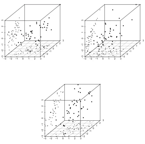
−3 −2 −1 0 1 2 3 −3 −2 −1 0 1 2 3 −3 −2 −1 0 1 2 3 ● ● ● ● ● ● ● ● ● ● ● ● ● ● ● ● ● ● ● ● ● ● ● ● ● ● ● ● ● ●● ● ● ● ● ● ● ● ● ● ● ● ● ● ●● ● ● ● ● ● ● ● ● ● ● ● ● ● ● ● ● ● ● ● ● ● ● ● ● ● ● ● ● ● ● ● ● ● ● ● ● ● ● ● ● ● ● ● ● ● ● ● ● ● ● ● ● ● ● ● ● ● ● ● ● ● ● ● ● ● ● ● ● ● ● ● ● ● ● ● ● ● ● ● ● ● ● ● ● ● ● ● ● ● ● ● ● ● ● ● ● ● ● ● ● ● ● ● ● ● −3 −2 −1 0 1 2 3 −3 −2 −1 0 1 2 3 −3 −2 −1 0 1 2 3 ● ● ● ● ● ● ● ● ● ● ● ● ● ● ● ● ● ● ● ● ● ● ● ● ● ● ● ● ● ● ● ● ● ● ● ● ● ● ● ● ● ● ● ● ● ● ● ● ● ● ● ● ● ● ● ● ● ● ● ● ● ● ● ● ● ● ● ● ● ● ● ● ● ● ● ● ● ● ● ● ● ● ● ● ● ● ● ● ● ● ● ● ● ● ● ● ● ● ● ● ● ● ● ● ● ● ● ● ● ● ● ● ● ● ● ● ● ● ● ● ● ● ● ● ● ● ● ● ● ● ● ● ● ● ● ● ● ● ● ● ● ● ● ● ● ● ● ● ● ● ● −3 −2 −1 0 1 2 3 −3 −2 −1 0 1 2 3 −3 −2 −1 0 1 2 3 ● ● ● ● ● ● ● ● ● ● ● ● ● ● ● ● ● ●● ● ● ● ● ● ● ● ● ● ● ● ● ● ● ● ● ● ● ● ● ● ● ● ● ● ● ● ● ● ● ● ● ● ● ● ● ●● ● ● ● ● ● ● ● ● ● ● ● ● ● ● ● ● ● ● ● ● ● ● ● ● ● ● ● ● ● ● ● ● ● ● ● ● ● ● ● ● ● ● ● ● ● ● ● ● ● ● ● ● ● ● ● ● ● ● ● ● ● ● ● ● ● ● ● ● ● ● ● ● ● ● ● ● ● ● ● ● ● ● ● ● ● ● ● ● ● ● ● ● ● ●

Figure 5: Samples of size n = 50 from C0.25(·), Cθ(0.75){Cθ(0.50)(u1, u2), u3} and

Gaus-sian copula with upper diagonal elements of the correlation matrix given by ρ = (0.25,0.25,0.75)⊤

(22)

From each copula we simulate a sample of n= 50 or n = 150 observations with standard normal margins. The margins are then estimated parametrically (normal distribution with estimated mean and variance) or nonparametrically. Respective columns in the tables are marked by “par.” and “emp.”. For each sample we estimate the AC using inference for the margins method, HAC using Okhrin et al. (2008) and the Gaussian copula using the generalised method of moments. Then we test how good these distributions ﬁt the sample. The empirical copula for both tests has been calculated as in (8). Number of bootstrap steps provided for the tests is equal to N = 1000. To sum up the simulation procedure, we used

1. F : two methods of estimation of margins (parametric and nonparametric);

2. C0 : hypothesised copula models under H0 (three models);

3. C : copula model from which the data were generated (three models with 3, 3 and 15 levels of dependence respectively);

4. n: size of each sample drawn from C (two possibilities, n = 50 and n= 150).

Thus, for all these 2×3×(3 + 3 + 15)×2 = 252 situations we perform 100 repetitions in order to calculate the power of both tests. This study is hardly comparable to other similar studies, because, as far as we know, this is the only one that considers the three dimensional case, and the only one that considers a hierarchical Archimedean copulae.

To understand the numbers in the tables more deeply let us consider ﬁrst the value in Table 1. The number 0.88 says, that testing using Kolmogorov-Smirnov type statistic

Tn for the AC with τ = 0.25 from the sample of a size n = 50, with nonparametrically

estimated margins, rejects the null hypothesesH0, assuming that the data are from HAC,

in 100%−88% = 12% of chances. It is very natural that the rejection rate for the AC, that have HAC under H0, is very close to the case, where AC is under H0. In general

AC is a special case of HAC. If the true distribution is AC, the rejection rates should be equal, or close to each other, and the diﬀerence based only on the estimation error.

Figure 6 represents the level of both goodness-of-fit tests for different sizes in terms of three quartiles; the outliers are marked with closed dots. In general, values lies below 0.1, which implies that the bootstrap performs well. Increasing the number of runs improves this graph. We see that if the sample size has enlarged three times, then the tests have approximately doubled their power in S statistics, and a slightly smaller coefficient is given for the T statistics. In general, small size samples from different models look very similar (see Figure 5), this makes detection of the model that best fits the data hardly applicable, this also explains a lot of outliers in Figure 6.

From the tables we see, that Sn performs, on average, better than Tn statistics, this can

be also seen from the Figure 6. In the tables, rejection rates for Sn under false H0 are in

general higher, than forTn statistics. We can also conclude that the larger the diﬀerence

between parameters of the model is the faster AC is rejected. This can be expressed by the only parameter in AC that does not covers the whole dependency.