XXX-X-XXXX-XXXX-X/XX/$XX.00 ©20XX IEEE
Application of Single Image Super-Resolution in Human Ear
Recognition Using Eigenvalues
Matthew Zarachoff
School of Computing, Creative Technologies & Engineering
Leeds Beckett University Leeds, United Kingdom
m.zarachoff4868 @student.leedsbeckett.ac.uk
Akbar Sheikh-Akbari
School of Computing, Creative Technologies & Engineering
Leeds Beckett University Leeds, United Kingdom [email protected]
Dorothy Monekosso
School of Computing, Creative Technologies & Engineering
Leeds Beckett University Leeds, United Kingdom [email protected]
Abstract— Ear recognition is a field in biometrics wherein images of the ears are used to identify individuals. Many techniques have been developed for ear recognition; however, most of the existing techniques have been tested on high-resolution images taken in a laboratory environment. This research examines the performance of Principal Component Analysis (PCA) based ear recognition in conjunction with super-resolution algorithms from low-super-resolution ear images. Ear images are first split into database and query images; the latter are first filtered and down-sampled, generating a set ear images of different low resolutions. The resulting low-resolution images are then enlarged to their original sizes using an assortment of neural network-based and statistical-based super-resolution methods. PCA is then applied to the images, generating their eigenvalues, which are used as features for matching. Experimental results on the images of a benchmark dataset show that the statistical-based super-resolution techniques, namely those that are wavelet-based, outperform other algorithms with respect to ear recognition accuracy.
Keywords— ear recognition; super-resolution; principal component analysis; eigenvalues
I. INTRODUCTION
Ear recognition is a field in biometrics wherein images of the ears are used to identify individuals. Ears are unique to individuals; even identical twins often have differentiable ears [1]. Application of ear recognition for security can be limited due to poor resolution of the images taken by surveillance cameras from a distance. Much research has been reported on ear recognition over the last two decades considering either mono or stereo images of ears [2-4]. While the effects of super-resolution on face recognition have been extensively studied [5–7], less has been reported about super-resolution on ear images.
This paper presents an investigation on the performance of ear recognition from low-resolution images using eigenvalues along with image super-resolution techniques. This is accomplished by utilizing several single image super-resolution techniques. The Principle Component Analysis (PCA) is then applied on the resulting enlarged image to calculate eigenvalues of the image. The eigenvalues are used to find the best match for the image within the dataset. Results show that ear recognition using the statistical based super-resolution techniques outperform the neural network based
methods. The rest of the paper is organized as follows: Section II introduces the state of the art ear recognition techniques, super-resolution methods and the proposed low-resolution ear recognition technique, including the benchmark ear image dataset. Section III presents the proposed evaluation method. Section IV describes the experimental results. Finally, Section V concludes the paper.
II. BACKGROUND AND METHODS A. Ear Recognition
Ear recognition techniques can be classified into several categories, including holistic and hybrid methods. Principal Component Analysis (PCA) and other related methods are examples of holistic techniques. These techniques basically extract some features from the ear image and use it as a basis for recognition [3-4]. Turk and Pentland [8] demonstrated the use of PCA on images of faces to perform facial recognition using the “eigenfaces” method. Victor, Bowyer, and Sarkar [4] later adopted the eigenfaces method on images of ears. They applied PCA based method reported in [8] to both face and ear images for comparative purposes. They reported that application of this PCA based method on facial recognition gives higher accuracy matching than that of the ear recognition, however, ears still demonstrated merit. Querencias-Uceta, Ríos-Sánchez, and Sánchez-Ávila [9] examined different distance measures for PCA based ear recognition methods to increase their accuracy. They assessed both Euclidean distance and Eigendistance to find the best match, concluding that Euclidean distance results in a higher accuracy. In addition, their investigation showed that flipping the image reduces the achieved accuracy and that increasing the number of training images increases the achieved accuracy. More recently, however, PCA and other linear transformation techniques have been used in conjunction with other feature extraction and classification methods to create hybrid classifiers [3,10-15]. A hybrid ear recognition method based on PCA and neural network was reported by Alaraj, Hou, and Fukami in [10]. This method applies PCA to a selected training set and extracts their principal components as in [4] to create a training matrix. It then creates a target matrix, which is a binary matrix, to indicate correct matches and it also normalizes both the training and target matrices. The training and target matrices are fed to a traditional multilayer feed-forward neural network to train the network. They have This research has been funded under a knowledge transfer partnership by
reported that the achieved recognition accuracy of their method is a function of the used number of training images per individual. Moreover, they showed that the use of a greater number of eigenvectors increases the achieved accuracy of the matching. Last but not least, their investigation determined that their algorithm generates superior results in terms of accuracy when using larger images. Zhang, Mu, Qu, Liu, and Zhang [11] compared the use of PCA with Independent Component Analysis (ICA), a similar method to PCA, to extract features from the ear images. The images are first filtered using either a Laplacian-Gaussian filter or a Weiner filter to create multiple experimental datasets. PCA is first used for feature reduction, then the ICA transform is applied to the resulting eigenvectors, generating a linear representation of the eigenvectors of ears. The resultant features are then classified via a three-layer Radial Basis Function (RBF) Network. They concluded that ICA based method outperforms the PCA based method in terms of the accuracy. Furthermore, they show that the application of Wiener filter results in a greater accuracy than use of the Laplacian-Gaussian filter and the use of either filter improves the performance of the identification method. Galdámez, Arrieta, and Ramón [12] used both Linear Discriminant Analysis (LDA) and Speeded-Up Robust Features (SURF) for ear recognition. LDA is similar transform to PCA except it utilizes Fisher’s linear discriminant than eigenvectors to create an earspace. This is accomplished in two steps; it first applies the standard PCA on the input images as in [4], creating their eigenvectors and consequently eigenears. It then calculates between-classes and within-classes matrices from the eigenears and uses them to create a dataset of projections. SURF is a scale and rotation invariant interest point detector and descriptor method used to extract key-points of an input image. The results of both LDA and SURF feature extraction are then fed to two three-layer feed-forward neural networks. Results demonstrated that SURF method outperforms the LDA algorithm and that both techniques give superior results to that of the PCA. Omara, Wu, Zhang, Du, and Zuo [13] reported a hybrid ear recognition technique using neural network, PCA and Support Vector Machine (SVM). They have applied VGG-M Net [16], a commonly used convolutional neural network for image recognition, on all input images, extracting image features. The number of features is then reduced through PCA. Both SVM and pairwise SVM were separately applied to the selected features to find the best match. Their results show that the application of pairwise SVM for finding the best match results in higher accuracy than that of the traditional SVM. Benzaoui and Boukrouche [14] introduced a feature extraction technique for ear recognition. They created a grayscale image separately for each ear image color component and they then applied three feature extraction methods called: Local Binary Patterns (LBP), Local Phase Quantization (LPQ) and Binarized Statistical Images Features (BSIF), to the resulting gray images, creating a histogram representation for each grayscale image. These three histograms, representing the ear features, are concatenated and then fed to the SVM classifier. Their experimental results show that BSIF technique generated the highest accuracy in finding the best match compared to LPQ and LBP methods.
B. Single Image Super-Resolution Techniques
Single Image Super-Resolution (SISR) is the process of increasing the resolution of a single image. Although this has been studied for several decades [17,18], SISR remains a challenging problem. Many SISR techniques have been successfully developed over the past two decades, including interpolation, neural networks [19-23] and statistical methods [24-29]. The methods used for this work are introduced here.
A convolutional neural network technique for image super-resolution was originally proposed by Dong, Loy, He, and Tang in [19]. The proposed method, called super-resolution convolutional neural network (SRCNN), is comprised of three convolution operations, where each operation uses a 2D filter of length nine, five and five, respectively. The output of each layer is also rectified. This technique uses the traditional backpropagation to train the network on patches of the input images. They reported superior results in comparison to the state of the art techniques at the time of its publication. Liu et al. [20] introduced the sparse coding based network (SCN) image enlargement algorithm. Their technique uses a Learned Iterative Shrinkage and Thresholding Algorithm (LISTA) in its network. In this technique, the input image is first up-sampled using the bicubic interpolation and then it will be split into a number of patches. Each resulting patch is then fed to the network, where its first layer is a convolutional layer. The output from this layer is then passed to a LISTA sub-network consisting of a finite number of recurrent stages to obtain a sparse code for the patch. The resulting sparse code is then multiplied with a high-resolution dictionary in a linear layer to generate the high-resolution representation of the input patch. The enlarged patches are finally reassembled generating the enlarged replica of the input image. They reported superior subjective and objective performance to SRCNN. Kim, Lee and Kyoung [21] proposed a neural network based super-resolution method, called: Very Deep Super Resolution (VDSR). This technique’s network has twenty layers, where all layers, except the first and the last layer, have 64 filters of size 3×3×64. Their technique splits the input image into a number of patches. The patches are then individually fed to the network, where the layer is just the input layer and the last layer is just a single filter of size 3×3×64. The VDSR technique attempts to predict the residual image, which is the difference between the low-resolution and high-resolution replica of the input image. They reported superior subjective and objective results compared to that of the SRCNN’s technique. In addition, their proposed VDSR method is faster than the SRCNN algorithm, despite its larger network depth. Tai, Yang, and Liu [22] introduced a deep neural network based super-resolution technique named: Deep Recursive Residual Network (DRRN), which comprises of residual and recursive units. Residual units were first introduced by He, Zhang, Ren, and Sun in [30]. They consist of two convolutional layers followed by a rectifier in series. They seek to learn the difference between their input and output, so that the overall output of the unit is the sum of the output of the convolutional layers and the original input. The recursive units are created using a series of residual units. The input to the recursive unit is first passed through a convolutional layer. The result is then passed to a residual unit. However, the results of that residual unit are passed to another residual unit to form a
cascade, with the results from the first convolutional layer being used by every residual unit in the recursive unit. The version of DRRN used for this paper is comprised of one recursive unit which contains nine residual units. Results show superior performance both qualitatively and quantitatively compared to VDSR. Sajjadi, Schölkopf, and Hirsch [23] proposed a neural network based algorithm for super-resolution. Their technique, Enhancenet, also seeks to learn the residual between low and high-resolution patches. Unlike previously discussed networks, Enhancenet does not use bicubic interpolation to up-sample the image prior to feeding it to the network. Instead, it uses the original, small low-resolution image. The network first passes the input patch through a convolutional layer followed by 10 residual blocks as in [30]. After the residual blocks, the patch is up-sampled 2x via nearest neighbor and fed to another convolutional layer. Another nearest neighbor/convolutional layer combination follows, with another convolutional layer and convolution operation after. This yields the residual component which is added to a bicubic up-sampling of the original patch to create the output. The authors also examined the effect of different loss functions when training the network. In addition to comparing mean square error (ENet-E) and perceptual loss (ENet-P), they examine each of those in combination with adversarial training (ENet-EA, ENet-PA) and texture loss (ENet-EAT, ENet-PAT). It was reported that ENet-E produces the highest Peak Signal-to-Noise Ratio (PSNR) of all training methods tested and that this outperformed state of the art methods at the time of publication, including SRCNN and VDSR. However, ENet-PAT demonstrated the highest qualitative performance per a survey of 49 individuals. This training method was also verified quantitatively by comparing up-sampled images from various training methods using image recognition. Images from the ImageNet dataset [31] were down-sampled by 4x and then up-sampled using Enhancenet with multiple training methods. These were then fed to ResNet-50 [24] for classification purposes. It was reported that ENet-PAT produced a lower Top-1 and Top-5 error when classifying the ImageNet dataset than other training methods.
Many wavelet-based statistical super-resolution methods have been reported in the literature [24-28]. Dumic et al. [24] reported a wavelet based super-resolution method. They enlarged the input image by first up-sample the input image and then applying the reconstructive wavelet filter on the rows and the columns of the resulting up-sample image. Dumic, Grgic, and Grgic reported superior subjective and objective visual quality to that of B-spline’s method. Temizel and Vlachos [25] introduced a wavelet based super-resolution method. They developed a method to estimate the LH and HL wavelet subbands’ coefficients of the low-resolution input image, while they assumed that the HH subband coefficients are zero and the low-resolution input image to be the baseband. This method assumes that the low-resolution input image is the low-low (LL0) subband of the high-resolution image to be
generated. It then calculates a HL0 like subband called: HL′0 by
applying the high-pass wavelet filter on the rows of the input image. It then applies a 2D non decimation wavelet transform on the input image converting it into its four subbands called: LL1, HL1, LH1, and HH1. It then applies a 1D high pass
wavelet filter on the rows of the resulting LL1 subband,
generating a 2D subband called: HL′1. The authors showed that
there is a strong correlation between coefficients of the HL1
and their respective four neighboring row coefficients in HL′1.
Hence, they introduced a linear least-squares regression approach to estimate HL1 from HL′1, calculating a set of
weights. The resulting weight are then used to generate an estimation for HL0 from HL′0. The same procedure was applied
on the LH′0 to generate an estimation for LH0. An inverse
wavelet transform is finally applied to LL0, HL0, LH0 and HH0,
which assumed to be set to zero. The authors reported significant higher objective quality in terms of PSNR in compared to those of the wavelet and Hidden Markov Model based techniques. Temizel and Vlachos [26] also developed a wavelet based super-resolution technique utilizing cycle spinning method. This technique assumes that the low-resolution input image to be the wavelet baseband of the target high-resolution image to be generated and its other subbands to be zero. It generates an initial high-resolution image called: by applying a 2D inverse wavelet transform on these subbands. Cycle spinning is then applied on the resulting initial high-resolution image, , generating the target super resolution image, as follows: a) it generates a number of 2D shifted replicas of ; b) it then applies a 2D wavelet decomposition on the resulting replicas; c) it generates a high-resolution of each replica by discarding its high frequency wavelet subbands and then performing 2D inverse wavelet transform on the resulting subbands; d) finally the high-resolution image is generated by averaging the realigned resulting high-resolution images. The authors reported superior objective quality in comparison with those of wavelet zero padding technique and other statistical based techniques. This technique was further expanded by the same authors in [27]. The new technique called: directional cycle spinning. This technique is first performed a 2D wavelet transform on the low-resolution input image to obtain its LH and HL subbands. It then partitions the input image into non-overlapping blocks. The horizontal and vertical activity measures for each block are then calculated by summing their respective wavelet coefficients in LH and HL subbands. Directional cycle spinning is then applied to the whole image in just horizontal and vertical directions, generating initial resolution image. The resulting high-resolution image is then adjusted by the activity measuring factors within each block. The authors showed that the directional cycle spinning outperforms the cycle spinning algorithm. Sheikh-Akbari and Bagheri Zadeh [28] introduced a wavelet based super resolution technique. This technique performs a 2D wavelet transform on the low-resolution input image dividing it into its wavelet subbands. It then applies reconstruction wavelet wavelet filters on the resulting high frequency subbands, accordingly, generating three high-resolution high frequency subbands. It then applies an inverse wavelet transform on the resulting high-resolution high frequency subbands and the low-resolution input image, which is assumed to be its wavelet baseband. The authors reported a superior performance with respect to both PSNR and the structural similarity (SSIM) criteria in comparison to those of cycle spinning, directional cycle spinning, and other statistical techniques. Another statistical based super resolution technique called: Regularization by Denoising (RED), was introduced by Romano, Elad, and Milanfar in [29]. This technique first
generates an initial high-resolution image from the low-resolution input image using bicubic interpolation. It then performs a gradient descent algorithm on the resulting image to minimize its noise using a Gaussian filter. The authors demonstrated a superior PSNR compared to those of the deblurring techniques.
III. PROPOSED EVALUATION METHOD
Principal Component Analysis (PCA) is a technique which is widely used to calculate an orthogonal basis for a dataset along which the variance is high. The orthonormal vectors forming this basis are known as eigenvectors and their scaling factors are eigenvalues. Let X be a 2D gray image of size m × n. The mean adjusted image X’ is created as follows:
X’ = X – XM (1)
where XM is the mean of all pixel values of the image. A
covariance matrix C is then calculated by:
C =X’X’T (2)
where C is of size m x m. The eigenvectors and eigenvalues of the matrix C are then calculated using the following decomposition:
C =ΕΛΕ Τ (3)
where the eigenvectors are the columns of E and the eigenvalues are the diagonal matrix values Λ=diag(λ1, λ2, ..., λn).
Gaidhane, Hote, and Singh [32] have used eigenvalues of facial images as features to classify emotions using a Levenberg–Marquardt based classifier algorithm. Further research reported in [4,15] have shown that Euclidean distance between the feature vectors of two ears is a sufficient measure to differentiate and match the ears. Consequently, in this research, Euclidean distance of the eigenvalues of two subject ear images is used as a criterion to assess their similarity. From the literature, it can be seen that much research has been conducted on the application of the PCA for ear recognition and also on still image super-resolution techniques.
Ear recognition has many real world applications, such as in forensics and video analytics. There is interest in using ear recognition techniques to identify individuals in public, however, images used for this purpose are often low resolution. To the authors’ knowledge, less research has been reported to assess the performance of the PCA for ear recognition in conjunction with super-resolution techniques. Consequently, there is a need to determine which super-resolution algorithms can be used effectively for this purpose. In this work, it is demonstrated that ear images having low resolution can be successfully used for ear recognition and examine which algorithms produce the most accurate results. Furthermore, results show that it is sufficient to use Euclidean distance of eigenvalues to match ear images.
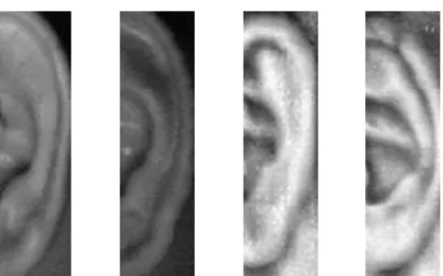
Fig. 1. Ear images from four individuals in the IITD II dataset. TABLE I. BLACKMAN 2DFIRFILTER COEFFICIENTS
0.0381 0.1051 0.0381
0.1051 0.4273 0.1051
0.0381 0.1051 0.0381
Fig. 2. Input high-resolution image and the resulting low-resolution images of factor 2, 4 and 8.
This investigation uses the Indian Institute of Technology Delhi Version 2 (IITD II) dataset [33]. This dataset consists of the images of the right ear of 221 participants. Each participant was photographed multiple times, with each image being of size 180 × 50 pixels and in 8-bit grayscale. Examples of ear images from the dataset can be seen in Fig. 1.
Two images for each subject were selected, with the set of first images forming a database. The second images serve as query images. The query images are passed through a Blackman 2D FIR low-pass filter to suppress the aliasing artifacts, as shown by Bagheri Zadeh and Sheikh-Akbari in [34]. The coefficients for the 3×3 filter are presented in Table 1. The Blackman 2D FIR low-pass filter has been shown to deliver perceptually higher visual quality images when used prior to down-sampling when compared to other smoothing methods.
After filtering, the query images are then down-sampled by a factor of 2. This process is repeated on the resulting image to further down-sample the images by factor of 4 and 8, resulting in image sizes of 90×25, 45×13, and 23×7, respectively. Examples of the resulting images are shown in Fig. 2.
The down-sampled images are then enlarged to their original size using both neural network and statistical based
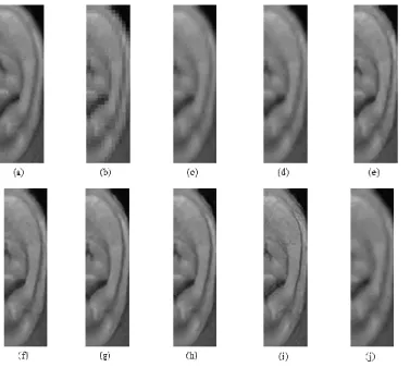
Fig. 3. Original high resolution image and its enlarged high resolution images: (a) high-resolution input ear image, (b) nearest neighbor, (c) bilinear interpolation, (d) bicubic interpolation, (e) SRCNN, (f) SCN, (g) VDSR, (h) DRRN, (i) Enhancenet, (j) Dumic et al., (k) Temizel and Vlachos, (l) Cycle Spinning, (m) Directional Cycle Spinning, (n) Sheikh-Akbari and Bagheri Zadeh, (o) RED and (p) 2D sinc super-resolution techniques.
Fig. 4. The image pipeline for query images.
single image super-resolution algorithms. A sample of all super-resolution techniques’ images used in this work are shown in Fig. 3.
Principal Component Analysis (PCA) is then performed on each image from both the database and the query image set to obtain its eigenvalues. The eigenvalues for each query image are then compared against the eigenvalues from all database images to find the best match using Euclidean distance. The overall process is illustrated in Fig. 4.
IV. EXPERIMENTAL RESULTS
The number of correct matches was calculated for each algorithm. If a query image was correctly matched with a database image, the test image was marked as a Top-1 image. If a query image was correctly matched with any one of the closest five database images, the query image was marked as a Top-5 image.
The matching results are tabulated in Table 2 for all three super-resolution cases (2, 4 and 8) as well as the averages of the statistical based methods and neural network based methods. The percentage of correctly matched 1 and Top-5 images is listed for each algorithm. The most accurate
TABLE II. TOP-1 AND TOP-5 MATCHES FOR ENHANCED EAR IMAGES USING VARIOUS SUPER-RESOLUTION TECHNIQUES
Table Head 2x Super-Resolution 4x Super-Resolution 8x Super-Resolution
Top-1 Top-5 Top-1 Top-5 Top-1 Top-5
Nearest 28.05 50.23 20.81 43.44 6.79 27.60 Bilinear 26.70 48.87 19.46 40.72 2.71 09.50 Bicubic 28.05 50.23 19.46 46.15 4.52 20.81 SRCNN [19] 26.70 50.68 20.36 40.27 10.86 33.48 SCN [20] 28.05 50.23 22.62 45.70 7.69 29.86 VDSR [21] 27.60 50.23 20.36 39.82 11.76 33.48 DRRN [22] 29.41 51.13 22.17 42.53 11.31 32.58 Enhancenet [23] [] [] 19.91 42.99 [] [] Dumic [24] 28.96 50.23 28.05 50.23 17.65 42.08 Temizel [25] 29.41 50.23 28.05 49.77 18.10 41.18 Cycle-Spin [26] 28.96 50.23 27.15 49.77 11.76 33.94 Dir. CS [27] 28.96 50.23 27.60 49.77 12.22 35.75 Sheikh-Akbari [28] 28.96 50.23 28.05 50.23 17.65 42.08 RED 28.51 50.23 19.46 46.15 4.52 20.81 sinc2 28.96 49.77 24.43 48.42 5.43 29.41 Statistical Avg 28.96 50.17 26.24 49.26 12.39 34.90 Neural Network Avg 27.94 50.57 21.09 42.26 10.41 32.35 classification for each is represented in bold. Enhancenet [23] was only used in the 4x case, as the model provided by the authors was only trained to perform 4x super-resolution. Nearest neighbor, bilinear interpolation and bicubic interpolation are excluded from the statistical method averages.
V. CONCLUSION
The efficacy of several single image super-resolution algorithms for the ear recognition problem has been presented in this paper. For images that are only somewhat low resolution, exemplified by the 2x down-sample case tested, most super-resolution algorithms work equally well. At lower resolutions, however, the statistical methods evaluated as part of this investigation produce the high resolution ear images which have eigenvalues closest to their original counterparts. Of particular interest was the success of wavelet-based techniques. Oddly, the wavelet-based techniques that were the most successful for matching did not produce superior visual quality images when compared to the neural network methods; this result could serve as a further line of investigation. In addition, the use of wavelet-based image enlargement techniques should be utilized with ear recognition methods aside from eigenvalue matching in future work.
ACKNOWLEDGMENT
This research has been funded under a knowledge transfer partnership by Innovate UK.
REFERENCES
[1] H. Nejati, L. Zhang, T. Sim, E. Martinez-Marroquin, and G. Dong, “Wonder ears: Identification of identical twins from ear images,” in
Proceedings of the 21st International Conference on Pattern Recognition (ICPR2012), 2012, pp. 1201–1204.
[2] A. Pflug and C. Busch, “Ear biometrics: a survey of detection, feature extraction and recognition methods,” IET Biometrics, vol. 1, no. 2, pp. 114–129, Jun. 2012.
[3] Ž. Emeršič, V. Štruc, and P. Peer, “Ear recognition: More than a survey,” Neurocomputing, vol. 255, pp. 26–39, Sep. 2017.
[4] B. Victor, K. Bowyer, and S. Sarkar, “An evaluation of face and ear biometrics,” in Object recognition supported by user interaction for service robots, 2002, vol. 1, pp. 429–432 vol.1.
[5] J. Jiang, C. Chen, J. Ma, Z. Wang, Z. Wang, and R. Hu, “SRLSP: A Face Image Super-Resolution Algorithm Using Smooth Regression With Local Structure Prior,” IEEE Transactions on Multimedia, vol. 19, no. 1, pp. 27–40, Jan. 2017.
[6] N. R. Roshna and S. Naveen, “Multimodal low resolution face recognition using SVD,” 2017, pp. 1–4.
[7] Z. Wang, Z. Miao, Q. M. Jonathan Wu, Y. Wan, and Z. Tang, “Low-resolution face recognition: a review,” Vis Comput, vol. 30, no. 4, pp. 359–386, Apr. 2014.
[8] M. A. Turk and A. P. Pentland, “Face recognition using eigenfaces,” in 1991 IEEE Computer Society Conference on Computer Vision and Pattern Recognition Proceedings, 1991, pp. 586–591.
[9] D. Querencias-Uceta, B. Ríos-Sánchez, and C. Sánchez-Ávila, “Principal component analysis for ear-based biometric verification,” in
2017 International Carnahan Conference on Security Technology (ICCST), 2017, pp. 1–6.
[10] M. Alaraj, J. Hou, and T. Fukami, “A neural network based human identification framework using ear images,” in TENCON 2010 - 2010 IEEE Region 10 Conference, 2010, pp. 1595–1600.
[11] H.-J. Zhang, Z.-C. Mu, W. Qu, L.-M. Liu, and C.-Y. Zhang, “A novel approach for ear recognition based on ICA and RBF network,” in 2005 International Conference on Machine Learning and Cybernetics, 2005, vol. 7, p. 4511–4515 Vol. 7.
[12] P. L. Galdámez, A. G. Arrieta, and M. R. Ramón, “Ear recognition using a hybrid approach based on neural networks,” in 17th International Conference on Information Fusion (FUSION), 2014, pp. 1–6.
[13] I. Omara, X. Wu, H. Zhang, Y. Du, and W. Zuo, “Learning pairwise SVM on deep features for ear recognition,” in 2017 IEEE/ACIS 16th International Conference on Computer and Information Science (ICIS), 2017, pp. 341–346.
[14] A. Benzaoui and A. Boukrouche, “Ear recognition using local color texture descriptors from one sample image per person,” in 2017 4th International Conference on Control, Decision and Information Technologies (CoDIT), 2017, pp. 0827–0832.
[15] L. Ghoualmi, A. Draa, and S. Chikhi, “An ear biometric system based on artificial bees and the scale invariant feature transform,” Expert Systems with Applications, vol. 57, pp. 49–61, Sep. 2016.
[16] K. Chatfield, K. Simonyan, A. Vedaldi, and A. Zisserman, “Return of the Devil in the Details: Delving Deep into Convolutional Nets,”
arXiv:1405.3531 [cs], May 2014.
[17] C. E. Duchon, “Lanczos Filtering in One and Two Dimensions,”
Journal of Applied Meteorology, vol. 18, no. 8, pp. 1016–1022, Aug. 1979.
[18] M. Irani and S. Peleg, “Improving resolution by image registration,”
CVGIP: Graphical Models and Image Processing, vol. 53, no. 3, pp. 231–239, 1991.
[19] C. Dong, C. C. Loy, K. He, and X. Tang, “Image Super-Resolution Using Deep Convolutional Networks,” IEEE Transactions on Pattern Analysis and Machine Intelligence, vol. 38, no. 2, pp. 295–307, Feb. 2016.
[20] D. Liu, Z. Wang, B. Wen, J. Yang, W. Han, and T. S. Huang, “Robust Single Image Super-Resolution via Deep Networks With Sparse Prior,”
IEEE Transactions on Image Processing, vol. 25, no. 7, pp. 3194–3207, 2016.
[21] J. Kim, J. K. Lee, and M. L. Kyoung, “Accurate Image Super-Resolution Using Very Deep Convolutional Networks,” in Proc. of IEEE Conference on Computer Vision and Pattern Recognition (CVPR), 2016.
[22] Y. Tai, J. Yang, and X. Liu, “Image Super-Resolution via Deep Recursive Residual Network,” in Proceedings of the IEEE Conference on Computer Vision and Pattern Recognition, 2017.
[23] M. S. M. Sajjadi, B. Schölkopf, and M. Hirsch, “EnhanceNet: Single Image Super-Resolution through Automated Texture Synthesis,” CoRR, vol. abs/1612.07919, 2016.
[24] E. Dumic, S. Grgic, and M. Grgic, “Image Interpolation Method Based on Wavelets,” in 2007 14th International Workshop on Systems, Signals and Image Processing and 6th EURASIP Conference focused on Speech and Image Processing, Multimedia Communications and Services, 2007, pp. 110–113.
[25] A. Temizel and T. Vlachos, “Wavelet domain image resolution enhancement,” IEE Proceedings - Vision, Image, and Signal Processing, vol. 153, no. 1, p. 25, 2006.
[26] A. Temizel and T. Vlachos, “Wavelet domain image resolution enhancement using cycle-spinning,” Electronics Letters, vol. 41, no. 3, pp. 119–121, Feb. 2005.
[27] A. Temizel and T. Vlachos, “Image resolution upscaling in the wavelet domain using directional cycle spinning,” J. Electronic Imaging, vol. 14, p. 040501, Oct. 2005.
[28] A. Sheikh-Akbari and P. B. Zadeh, “Wavelet Based Image Enlargement Technique,” in Global Security, Safety and Sustainability: Tomorrow’s Challenges of Cyber Security, 2015, pp. 182–188.
[29] Y. Romano, M. Elad, and P. Milanfar, “The Little Engine That Could: Regularization by Denoising (RED),” SIAM Journal on Imaging Sciences, vol. 10, no. 4, pp. 1804–1844, Jan. 2017.
[30] K. He, X. Zhang, S. Ren, and J. Sun, “Deep Residual Learning for Image Recognition,” in 2016 IEEE Conference on Computer Vision and Pattern Recognition (CVPR), 2016, pp. 770–778.
[31] O. Russakovsky et al., “ImageNet Large Scale Visual Recognition Challenge,” Int J Comput Vis, vol. 115, no. 3, pp. 211–252, Dec. 2015. [32] V. H. Gaidhane, Y. V. Hote, and V. Singh, “Emotion recognition using
eigenvalues and Levenberg–Marquardt algorithm-based classifier,”
Sadhana, vol. 41, no. 4, pp. 415–423, Apr. 2016.
[33] “IIT Delhi Ear Database.” [Online]. Available: http://www4.comp.polyu.edu.hk/~csajaykr/IITD/Database_Ear.htm. [Accessed: 13-Mar-2018].
[34] P. B. Zadeh and A. Sheikh-Akbari, “Image resolution enhancement using multi-wavelet and cycle-spinning,” in Proceedings of 2012 UKACC International Conference on Control, 2012, pp. 789–792.