Proceedings of the 2014 International Conference on Industrial Engineering and Operations Management Bali, Indonesia, January 7 – 9, 2014
1070
A Technical Note on the Single-Vendor Multi-Buyer Integrated
Inventory Supply Chain Problem
Md Abdul Hoque
Universiti Brunei Darussalam
Brunei Darussalam
Abstract
Recently two single-vendor multi-buyer integrated inventory models were developed by incorporating some realistic factors. The production flow was synchronized by transferring the lot with equal- and/or -unequal sized batches (sub-lots), where the equal-sized batches were kept to be equal to the largest unequal-sized batch. A common minimal total cost solution technique to the models was derived, and its potential significances were highlighted with solutions of some numerical problems. Because of the inflexible restriction on the equal-sized batches in the models, they failed to provide the generalized minimal total cost solution to a single-vendor single-buyer numerical problem. Here we extend the models by restricting the equal-sized batches to be less than or equal to the largest unequal-sized batch multiplied by the ratio of the production rate to the total demand rate, as used in another recently published research work. Then we derive a different simplified common solution method to the extended models. Thus the key contribution of this paper is the extension of these recently developed models to more generalized ones and development of a simple common solution technique to them. The potential significance of this extension is reported with the solutions of some numerical problems. The key research contribution of this paper is the extension of two recently developed single-vendor multi-buyer integrated inventory models to more generalized ones and development of a simple common solution technique to them.
Keywords
Single-vendor multi-buyer, integrated inventory, equal-sized batches, minimal total cost.
1. Introduction
The single-vendor multi-buyer integrated inventory supply chain in meeting deterministic demand has received a considerable attention of the researchers (Vide for detail Hoque (2008, 2011a, 2011b), Sarker and Diponegoro (2009), Zavanella and Zanoni (2009, 2010); Srinivas and Rao (2010), Glock (2012), Kim and Goyal (2012), Ben-Daya et al. (2013)). Unlike others, Hoque (2011a, 2011b) synchronized the integrated production flow by transferring the lot with equal- and/or -unequal sized batches. In both cases the next unequal-sized batch is a multiple of the previous one by the ratio k of the production rate to the total demand rate. In Hoque (2011a) the equal-sized batches are flexibly restricted to be less than or equal to the largest unequal-sized batch multiplied by k, while in the latter the equal-sized batches are inflexibly restricted to be equal to the largest unequal-sized batch. Because of this inflexible constraint on equal-sized batches in Hoque (2011b), the solution technique there leads to a higher minimal total cost solution for a single-vendor single-buyer numerical problem, originally solved by Hill (1999) and recently by Hoque (2011a), developed following the synchronization approach in Hill (1999). Although Hoque (2011b) failed to show the generalized characteristic in obtaining the minimal total cost solution for that problem, it has coped with relaxations of some impractical assumptions, such as insignificant set up and transportation times, unlimited capacities of the transport equipment and buyers’ storage, unrestricted lead time of supplying a batch and the boundless smallest batch size, which have not been considered in Hoque (2011a). Therefore, here we extend the models in Hoque (2011b) by taking advantage of the flexible restriction on the equal-sized batches in synchronizing the production flow as in Hoque (2011a), but retaining the realistic factors as considered in Hoque (2011b). In the current models the smallest batch size to each of the buyers is restricted to be greater than or equal to one (in case of bulk materials, the desired smallest amount of a material can be assumed as 1 unit) as in Hoque (2011b). The equal-sized batches to each of the buyers are kept to be greater than or equal to one but less than or equal to the respective largest unequal-sized batch size multiplied by k. Then a different common simple solution method to the extended models is presented. Thus the simple solution method to the integrated vendor-buyers problem with a flexible restriction on the equal sized batches, but satisfying the constraints for relaxations of the mentioned impractical assumptions is more effective than the previous ones. The potential
1071
significance of the new method of solution to the problem, and the effects of the mentioned factors on the minimal total cost solution are shown with solutions of some numerical problems.
The outline of the remainder of the paper is as follows: Section 2 deals with assumptions and notations, and then presentation of the models and their minimal total cost solution methods. This follows a section of solutions to numerical problems and comparative studies of the concerned methods on their results. The last section finishes with discussion and conclusion.
2. Formulation of the Extended Models
2.1 Assumptions and NotationsThe assumptions and notations are the same as used in Hoque (2011b) except some additional notations. The notations are as follows:
For the vendor
D Annual rate of demand; P Annual rate of production (P > D and k = P/D); h Inventory carrying cost per item per year; S Production set up cost per lot; s1 Set up time (in yr); z The smallest batch (part of a lot) size;
y The equal- sized batch from the vendor; gv Capacity of the vendor’s storage Q The lot size transferred from the vendor to the buyers
n Total number of equal- and/or -unequal sized batches in a lot; e Number of unequal-sized batches in a lot(en);
h
L The largest lead time; Ls The smallest lead time. For the ith buyer (i = 1, 2,...,m);
Di Annual rate of demand,
m
i Di
D 1 ; Ti Cost of shifting a batch from the vendor; hi Inventory carrying cost per item per year; si Cost of placing an order of a lot; yi the equal sized batch to the buyer;
g
i,t Capacity of the transport vehicle;s i
g
, Capacity of the buyer’s storage(gi,s gi,t);
m i it v g g 1 , ) ( 1 , i
t Inspection, loading, transfer and unloading time (in yr);
2 ,
i
t Return time of the transport vehicle (in yr); zi The smallest batch size;
2.2 Model I and its solution method
(
Assuming a batch transfer just after finishing its
processing)
2.2.1 The total cost function
The vendor transfers the lot Q to the buyers in e unequal sized batches of sizes z,kz,k2z,...,ke1z and n-e equal sized batches of size y (y = z if e = 1; y = 0 if n = e; otherwisez ykez)such that
; / 1 1z Dk z D k j i i j D y D yi i / for j = 1,2,…e; i = 1,2,…,m and ; 1 1 1
m i i j j z k zk kjz/Pkj1zi/Di kj1z/Dfor j=1,2,…,e-1. Thus Q y e n z k z k kz z 2 ... e1 ( )
1 0 / ) ( er r k y e n Q z (1) Following Model I of Hoque (2011b) but replacing the repeated batchk
e1z
by y, the repeated batch here and simplifying find the joint total cost per year as follows:
) 1 ( ) 1 ( ) 1 ( ) 1 )( ( ) 1 )( 1 ( 2 ) 1 )( 1 ( ) 1 ( 2 ) 1 )( 1 ( k k h h h k k y k e n Q k k k k k h h k k h k k e e e e e e
, 2 ) ( 1 ) 1 )( 1 ( ) 1 )( 1 )( ( ) ( 1 1 ,1 2
m i i ii e e t h D k h h y e n k k k k e n nA S D Q where
m i i m i i m i Dihi D S S S A T h 1 / ; 1 ; 1 . (2)1072 2.2.2 The constraints
The capacity constraint on the transport vehicle as given in Hoque (2011b) is g z ke1 ; ) / ( Min i,t i i Dg D g [ / ,] 1 t i e ik z D g D (3) Substituting for z from (1) and simplifying it leads to
) ( 1 0k n e y g Q e r r
(4) Also, yigi,tyg[yi Diy/D] (5)In case of transferring the repeated batch, y instead of
k
e1z
used in Hoque (2011b) and following the logical arguments there obtaine i i is g D y k D e n D zD k 1 , / ) / 1 1 ( ) ( / (6)
Substituting for z from (1) and simplifying it transforms to
1 0 , ) ( e r r i s i e k D Dg k y e n Q (7) Sinceg, Dk 1z/D, e i t i so 1 . 1g, k z g m e i it v
Similarly, gv y can be shown.Following Hoque (2011b) the lead time, the set up time, the transfer time and the smallest batch size constraints are respectively, given by e1ln(Lh/Ls)/lnk (8) ) 1 /( 1 ) / 1 / 1 /( 1 s D P kDs k Q (9) ) ( /D ti,1 ti,2 z and zi 1zD/Di
Substituting for z from (1) into the last two constraints, and simplifying derive
) ( Max ), / 1 ( Max ), , ( Max ; ) ( ,1 ,2 1 0 i i i i i e r r t t t D t t t t k t D y e n Q
(10) Alsoykez. Substituting for z from (1) and simplifying obtain
n e k k k
yQ ( )( e1)/ e( 1) (11) Therefore, the mathematical model of the problem is to minimize the total cost function (2) subject to the constraints (1), (4), (5), (7), (8), (9), (10) and (11).
2.2.3. Solution Technique
Case I When e = 1 (the lot is transferred only with equal sized batches)
In this case y = z and hence from (1) Q = nz and the joint total cost function transforms to
m i Dihiti z D A n S k h k n h h z 1 ,1 2 ) 1 ( Given z, the minimizing n can be obtained as
k
h S Dk z z n 1 2 1 ) ( (12a)Substituting this value of n(z) in the total cost function, it transforms to 2 ( 1) , 2 ) ( 1 ,1
m i Dihiti z AD k k h S D k h h zwhich is convex in z. The minimizing z is given by h h kAD z 2 (12b) For this value of z, minimizing n(z) can be calculated from (12a). However, the realistic feasible solution can be found by satisfying the following inequalities obtained from constraints (3), (6), (9) and (10) (constraint (11) is always true).
, 1/{ ( 1)}
Min
, /[ { (1 1/ ) 1/ }]
Max DtkDs n k z g Dgi,s Di n k k (13) So, for the obtained minimizing z from (12b), calculate the minimizing n(z) from (12a). If either the rounding down or the rounding up values of n (if n(z) < 1, set n =1) satisfies (13), then for the minimizing z from (12b), decide the minimal total cost by calculating the total cost at the rounding down or the rounding up values of n. If the left hand side inequality in (13) is not satisfied, it may be satisfied by increasing the rounding up value of n(z) by 1 at each
1073
step. The smallest of the integral values of n that satisfies (13) is the minimizing n in this case. If the right hand side inequality in (13) is not satisfied, it may be satisfied by decreasing the rounding down value of n(z) by 1 at each step. The largest of the integral values of n that satisfies (13) is the minimizing n. If an integral n satisfying (13) does not exist, then the problem is infeasible. Otherwise, calculate the value of Q from (1) for known e, n and hence the minimal total cost from (2).
Case II When n = e or y = 0 (the lot is transferred only with unequal sized batches) Considering the total cost function (2), the minimizing Q is given by
) )( 1 )( 1 ( ) 1 )( 1 ( 2 ) ( h k h k k D nA S k k k n Q n n (14) So, for each of the feasible values of e satisfying (8), set n = e and calculate the minimizing feasible Q (if exists) by satisfying the following inequalities obtained from constraints (4), (9), (10) and hence the minimal total cost from (2).
1/( 1),
Max 1 0 1 0
n r r n r r Q g k k t D k kDs (15) The minimum of the minimal total costs obtained for feasible values of e satisfying (8) along with the associated values of Q and n = e leads to the final minimal total cost solution in this case.Case III When n > e and yz Sub-case 1 Whenhh
In this case, given n, e and y, the minimizing Q, denoted by Qmin,is given by
) 1 )( 1 ( 2 ) 1 )( 1 ( ) 1 ( 2 ) 1 )( 1 ( 2 ) ( 1 ) 1 )( 1 ( ) 1 )( 1 )( ( ) ( ; / 1 2 1 1 1 min e e e e e e k k k k k h h k k h k k B k h h y e n k k k k e n nA S D A B A Q (17)The feasible minimizing Q satisfying the constraint H1Qmin H2(if exists), where H1 is the maximum of the right hand sides of (9), (10), (11) and H2 is the minimum of the right hand sides of (4) and (7), can be obtained and hence the associated total cost from (2).
Again, given Q, n and e, the minimizing y, denoted by
y
min is given as follows:
kQ h h e n k k k k e n B k k h h h k k k e n A B A y e e e e e ) ( 1 ) 1 )( 1 ( ) 1 )( 1 )( ( 1 ) 1 ( 1 ) 1 )( ( ; / 2 2 2 2 min (18)The feasible
y
min has to satisfy constraints (4), (5), (7), (10) and (11), that is,
g k k k e n k Qk e n k t D Q y e n D k Dg Qk e n k g Q e e e e r r i e r r s i e e r r , ) 1 ( ) 1 ( ) ( ) 1 ( , Min / , Max 1 0 min 1 0 , 1 0 Note that 0, 1 0
e r r k t DQ otherwise after substituting for Q from (1) leads to a contradiction zDt. Thus for known e, n and Q, the minimizing y can be calculated from (18). The feasible minimizing
, 1/{ ( 1)}
Max
z Dt kDs nk
y by satisfying the above inequalities (if exists) can be found and hence the associated total cost from (2). Similarly, given Q, y and e, the minimizing n, denoted by
n
min is given by) 1 )( 1 ( ) 1 )( 1 ( 5 . 0 ) ( ) 1 )( ( ) 1 ( 2 min e ee k k k k h h y DAk y Q k h h y k h Q e n (19) The feasible nmin needs to satisfy constraints (4), (7), (10) and (11), that is,
y Q k k k e y k t D Q e n y D k Dg Qk e y k g Q e e e e r r i e r r s i e e r r ) 1 ( 1 , Min / , Max 1 0 min 1 0 , 1 01074 Note that 1 1 1 ... 1 0 ) 1 ( 1 1 ee e k k k e k k k
e for
e
1
and hence for e2. So, for given Q, y and e, the minimizing integral n can be calculated as the rounding up or rounding down values of nmin obtained from (19). The feasible minimizing n e1 (if exists) can be determined by satisfying the inequalities above.Sub-case 2 Whenhh
The coefficient of Q in (2) is positive. Otherwise, non-positive coefficient of Q in (2) implies
1
2 0 1 0 2 1 0 2 1 2 ) 1 ( 1
e r r e r r e r r k k k h h k k k k
1 0 1 0 2 1 0 2 1 2 1 1 e r r e r r e r r k k h h k k
) 1 ( 1 1 2 1 2 ) 1 ( 2 2 1 1 0 1 0 1 0 2 1 0 1 0 2 e e e r r e r r e r r e r r e r r k k k k k k k k h k h , 2 1 2 ) 1 ( 2 1 2 1 2 ) 1 ( 1 1 2 1 2 1 1 0 1 0 2
e e e e e r r e r r k k k k k k h k h a contradiction.In case ofhh, the feasible minimizing Q can be determined following the procedure as in Sub-case 1 of Case III for determining the same. Observe that the total cost function is a decreasing function in y, given Q, n and e, and hence the minimal y is at its highest available feasible value in the range provided earlier. Also for given Q, e and y, the total cost function (2) is decreasing in n if 0,
) 1 ( ) 1 ( e k k y k Q
A and hence the minimal n is at its highest available
feasible value in the range provided earlier; otherwise, the minimal n is at its least available feasible value in that range. In case of hh,observe that for given Q, n and e the total cost function (2) is concave in y (assuming y as real), and for given Q, e and y it is also concave in n (assuming n as real), and hence respective minimizing y and n is at its least or highest feasible value. Thus for given Q, n and e the total cost function has its minimal value either at y = z or at the highest value of its feasible range as provided earlier. Also, for given Q, e and y the total cost function has its minimal value either at n = e + 1 or at the highest value of its feasible range as provided earlier. For given n, e and y if the coefficient of 1/Q in the total cost function is non-positive, then it is concave in Q and so the minimizing Q exists either at the least value of z or at the highest value of Q at its feasible range as given earlier. Otherwise, the total cost function is convex and the minimizing Q is given by (17), and hence the feasible minimizing Q can be determined by following the process described in Sub-case 1.
Therefore, starting with known e satisfying (8), set n = e + 1, and yzMax
Dt,kDs1/{n(k1)}
[satisfying (9) and (10), (11) is always satisfied for y = z], the minimizing Q, Qminand hence the feasible minimizing Q can be calculated. Using that minimizing Q and known n and e, a feasible minimal value of y can be found. Again, for known Q, y and e, a feasible minimal integral value of n can be found. For known n, e and y the feasible minimizing Q can be calculated yet again. Iteration of this process of calculating minimizing Q, n and y leads to the minimal total cost solution to the problem. Minimum of the minimal total costs obtained for all feasible e satisfying (8), along with the associated values of Q, n, e and y leads to the final minimal total cost solution in this case.2.3 Model II and its Solution Method (Assuming a batch transfer when the previous batch
finishes at the buyers)
2.3.1 The total cost Function
Considering the batch sizes at the vendor and their distribution to the buyers as the same as in Model I, the value of z can be obtained as in (1). Then following Model II of Hoque (2011b) but replacing the repeated batch
k
e1z
by y and simplifying obtain the total cost per year as follows:
) 1 ( ) 1 ( ) 1 ( ) 1 )( ( ) 1 )( 1 ( 2 ) 1 )( 1 ( ) 1 ( 2 ) 1 )( 1 ( k k h h k h k y k e n Q k k k k k h h k k h k k e e e e e e
m i i e e t Dh h h y e n k k k k e n nA S D Q 1 ,1 2 2 ) ( 1 ) 1 )( 1 ( ) 1 )( 1 )( ( ) ( 1 (20)1075 2.3.2 The Constraints
All the constraints except the capacity constraint of the buyer’s storage are the same as in Model I. Here we consider the capacity constraint of the vendor’s storage since inventory is accumulated at the vendor. In case of transferring the repeated batches, first the batch
k
e1z
iis transferred to the buyer. This batch meets the demands for the time. / 1 D z k i e
In this time the manufacturer produces at most e i i e z k D z
Pk1 / units if required. After transferring yi units to the buyer i, i i
e
y z
k units remain at the vendor’s storage. These yi units finish at the buyer i in yi/D units of time. At this time the manufacturer can produce at most Pyi/D = kyi units if required. So the highest accumulated inventory at the manufacturer’s storage could be i ( 1) i.
e i i i e y k z k ky y z
k If the manufacturer continues to produce for the time yi/D, then the next accumulated highest inventory will be kezi2(k1)yi. In this way the highest accumulated inventory at the manufacturer’s storage for n-e repeated batch of yi units could be
, ) 1 )( 1 ( i i e y k e n z
k which must be less than or equal to
g
v,
i. e., v i i i e g D y D k e n D z D k / ( 1)( 1) / Substituting for z from (1) and simplifying it transforms to
1 0 ) 1 ( ) ( e r r i v e e e k kD Dg k y k k y e n Q (21) Since gi,t gi,s, so ke1zi gi,t gi,s; yi gi,t gi,s. 2.3.3 Solution Technique Case I When e = 1Substituting for y = z and Q = nz in (20) the joint total cost function transforms to
m i ti Dh z D A n S k h h h k h k n z 1 ,1 2 2 ) ( ) 1 (For
h
h
,
the coefficient of z is positive. For hh, it can also be shown that the coefficient of z is non-negative. Given z, the minimizing n is obtained as
k
h S Dk z z n 1 2 1 ) ( (22a) Substituting this value of n(z) in the total cost function and simplifying the minimizing z is given byh h h k kAD z 2 ) ( 2 (22b)
The minimal total cost solution to the problem can be obtained by following the solution procedure of Case I of Model I but using the total cost function developed here, formulas (22a), (22b) instead of (12a) and (12b) respectively and the constraint (21) instead of (7).
Case II When n = e or y = 0
In this case the total cost function can be transformed to the one as obtained in case II of Model I, and hence follows the same solution procedure there but using constraint (21) instead of constraint (7).
Case III When n > e and yz Sub-case 1 Whenhh
The coefficient of Q in (20) can be shown positive. Then denoting the coefficient of 1/Q and Q in (20) by
A
1
andB
1
respectively, the minimal Q, Qmincan be given as Qmin A1/B1. The feasible Qmincan be found by satisfying theconstraints H1Qmin H2,where H1is the maximum of the right hand sides of (9), (10), (11) and H2is the minimum of the right hand sides of (4) and (21. As in Sub-case 1 of Case III of Model I, the minimal y, ymin for known Q, n, and e is given by
2 2 min A /B y (22)
; 1 ) 1 ( 1 ) 1 )( ( 2 k k h h k h k k e n A e e
Q h h e n k k k k e n B e e 2 ) ( 1 ) 1 )( 1 ( ) 1 )( 1 )( ( 2 The feasible
y
min can be found by satisfying the following constraint (obtained from constraints (4), (5), (9), (10)1076
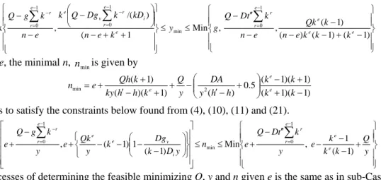
) 1 ( ) 1 ( ) ( ) 1 ( , , Min 1 ( ) /( , Max 1 0 min 1 0 1 0 e e e e r r e i e r r v e e r r k k k e n k Qk e n k t D Q g y k e n kD k Dg Q k e n k g QGiven Q, y and e, the minimal n, nminis given by
) 1 )( 1 ( ) 1 )( 1 ( 5 . 0 ) ( ) 1 )( ( ) 1 ( 2 min k k k k h h y DA y Q k h h ky k Qh e n e e e (23)
This
n
min needs to satisfy the constraints below found from (4), (10), (11) and (21).
y Q k k k e y k t D Q e n y D k Dg k y Qk e y k g Q e e e e r r i v e e e r r ) 1 ( 1 , Min ) 1 ( 1 ) 1 ( , Max 1 0 min 1 0Each of the processes of determining the feasible minimizing Q, y and n given e is the same as in sub-Case 1 of Case III of Model I, but requires the use of the formulas forQmin, ymin,
n
min and their feasible ranges derived in thissub-section.
Sub-case 2 Whenhh
Given e satisfying (8), the processes of determining the feasible minimizing Q, y and n are respectively the same as in sub-Case 2 of Case III of Model I, but using the objective function (20) and their feasible ranges developed here. Thus for a given set of values of the parameters of a problem, the minimal total cost solution by considering each of the cases of the Model I and Model II can be found. The least of them associated with the values of the variables is the final solution.
3. Numerical Illustration
Although Hoque (2011b) obtained the same minimal total cost solutions for three of the four vendor single-buyer numerical problems originally found by Hill (1999) and Hill and Omar (2006), it led to a higher minimal total cost solution for the remaining one originally solved by Hill (1999). These numerical problems are solved by the method developed in this paper, and each of the solutions is found to be the same as found originally. The numerical problem of supplying a product by a vendor to five buyers originally solved by Hoque (2011a, 2011b), is solved using the solution method developed in this paper. The current solution method provides the same least minimal total cost solution to this numerical problem as obtained by Hoque (2011a). Another single-vendor 5-buyer numerical problem originally solved by Hoque (2008) and then by Hoque (2011b) is also solved by applying the current method, and found to provide the same solution as obtained by them.
The method developed in this paper is also applied to solve the single vendor two-buyer numerical problem originally solved by Zavanella and Zanoni (2009). The data for the problem are as given in Table 1.
Table 1: Data for the single-vendor 2-buyer problem of Zavanella and Zanoni (2009)
1500 2 1
i DiD and no limit on each of Ls, Lh, gi,s, gi,t and gv. Comparative minimal total cost solutions are given in the Table 2.
Table 2: Comparative results for a single-vendor 2-buyer problem of Zavanella and Zanoni (2009)
*Z & Z denotes Zavanella and Zanoni
For vendor Buyer si Di hi Ti ti,1 ti,2
S P h 1 75 500 4 0 0 0 400 3200 5 2 25 1000 4 0 0 0
Method Model (n, e) & i
n Lot Size Batch Sizes from the vendor T. Cost
Z & Z* (2009) Joint Optimum n
1 = 1, n2 = 3 637.5 1x212.5+ 3x141.67 2585.70 Hoque (2011a) Model II (839, 1) 839 839x1 1787.47 Hoque (2011b) Model I (279, 1) 837.20 279x3 1791.70 This Paper Model I (280, 1) 840 280x3 1791.69
1077
Considering the realistic situation, the smallest batch sizes to the buyers are kept greater than or equal to one here and in Hoque (2011b), and hence they lead to the same minimal total cost solution. But such a constraint had not been imposed in Hoque (2011a), and hence it led to the least minimal total cost solution by distributing each batch of 1 unit released from the vendor to the buyers as follows. 1x500/1500 = 0.333... units to buyer 1 and 1x1000/1500 0.666… units to buyer 2. Recall that Model I of Hoque (2011b), Model II of Hoque (2011a) and Model I of this paper are developed by accumulating the inventory at the buyers, while Model II of Hoque (2011b), Model I of Hoque (2011a) and Model II of this paper are developed by accumulating the inventory at the vendor.
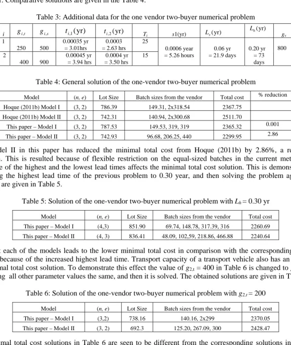
Thus the current solution method is found to lead to the least minimal total cost solutions to all the numerical problems studied. The previous single-vendor two-buyer numerical problem along with some additional parameter values as given in Table 3, originally solved by Hoque (2011b) is again solved by applying the method developed in this paper. Comparative solutions are given in the Table 4:
Table 3: Additional data for the one vendor two-buyer numerical problem
Table 4: General solution of the one-vendor two-buyer numerical problem
The Model II in this paper has reduced the minimal total cost from Hoque (2011b) by 2.86%, a reasonable reduction. This is resulted because of flexible restriction on the equal-sized batches in the current method. The difference of the highest and the lowest lead times affects the minimal total cost solution. This is demonstrated by increasing the highest lead time of the previous problem to 0.30 year, and then solving the problem again. The solutions are given in Table 5.
Table 5: Solution of the one-vendor two-buyer numerical problem with Lh= 0.30 yr
Note that each of the models leads to the lower minimal total cost in comparison with the corresponding costs in Table 4, because of the increased highest lead time. Transport capacity of a transport vehicle also has an effect on the minimal total cost solution. To demonstrate this effect the value of g2,t = 400 in Table 6 is changed to g2,t = 200
by keeping all other parameter values the same, and then it is solved. The obtained solutions are given in Table 6.
Table 6: Solution of the one-vendor two-buyer numerical problem with g2,t= 200
The minimal total cost solutions in Table 6 are seen to be different from the corresponding solutions in Table 4, demonstrating the effects of the lower transport capacity. Buyers’ storage capacity also affects the minimal total cost solution. To demonstrate this, the single-vendor two-buyer numerical problem is solved by replacing the values of g2,t and g2,s in Table 6 by 200 and 250 respectively but keeping all other parameter values the same. The solutions
are given in Table 7.
i gi,t gi,s ti,1(yr) ti,2(yr) Ti s1(yr) Ls(yr) ) yr ( h L gv 1 250 500 0.00035 yr = 3.01hrs 0.0003 = 2.63 hrs 25 0.0006 year = 5.26 hours 0.06 yr = 21.9 days 0.20 yr = 73 days 800 2 400 900 0.00045 yr = 3.94 hrs 0.0004 yr = 3.50 hrs 15
Model (n, e) Lot Size Batch sizes from the vendor Total cost % reduction Hoque (2011b) Model I (3, 2) 786.39 149.31, 2x318.54 2367.75
Hoque (2011b) Model II (3, 2) 742.31 140.94, 2x300.68 2511.70
This paper – Model I (3, 2) 787.53 149.53, 319, 319 2365.32 0.001 This paper – Model II (3, 2) 742.93 96.68, 206.25, 440 2299.95 2.86
Model (n, e) Lot Size Batch sizes from the vendor Total cost This paper – Model I (4,3) 851.90 69.74, 148.78, 317.39, 316 2260.69 This paper – Model II (4, 3) 836.41 48.09, 102,59, 218.86, 466.88 2240.64
Model (n, e) Lot Size Batch sizes from the vendor Total cost This paper – Model I (3,2) 738.16 140.16, 2x299 2370.05 This paper – Model II (3, 2) 692.3 125.20, 267.09, 300 2428.47
1078
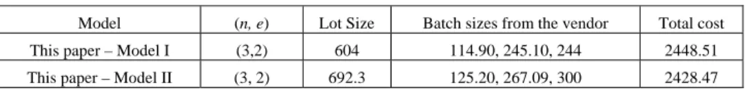
Table 7: Solution of the one-vendor two-buyer numerical problem with g2,s= 200
It can be noted from Table 6 and Table 7 that Model I leads to the lower minimal total cost solution because of more restriction on the second buyer’s storage capacity.
4. Discussion and Conclusion
Here we have extended two single-vendor multi-buyer models developed by Hoque (2011b), by incorporating the notion of synchronizing the production flow with a flexible restriction on the equal sized batches as in Hoque (2011a). In the latter one, two single-vendor multi-buyer models were developed by transferring the lot with equal- and/or -unequal sized batches, but the equal-sized batches were kept less than or equal to the largest unequal-sized batch multiplied by k. In these models he had not imposed any other constraint. But Hoque (2011b) presented two single-vendor multi-buyer models by transferring the lot with equal- and/or -unequal sized batches, in which the equal-sized batches were kept to be equal to the largest unequal-sized batch. The smallest batches to the buyers were also kept greater than or equal to one. Besides, constraints on the capacities of transport vehicles and buyers storages, the smallest and the highest lead times, set up and transportations times were imposed. Although the models in Hoque (2011a) are more generalized in respect of designing the batches to synchronize the production flow, they have not taken into account these realistic constraints. While the models in Hoque (2011b) are more realistic in respect of considering realistic constraints, but it lacks of synchronizing the production flow properly. Because of this lack of synchronization, it failed to lead to the generalized minimal total cost solution to a single-vendor single-buyer numerical problem as obtained by Hill (1999). So, the models in Hoque (2011b) have been extended here by transferring the lot with batches as in Hoque (2011a), but retaining the realistic constraints there. In addition, the capacity constraint on the vendor’s storage is imposed. Then a different common simple solution method to the models is developed. Following the solution method numerical problems are solved and comparative studies are carried out. The present method is found to provide the same solution to each of four single-vendor buyer numerical problems originally solved by Hill (1999) and Hill and Omar (2006). Also, two single-vendor five-buyer numerical problems originally solved by Hoque (2008) and then by Hoque (2011a), are solved by applying the method developed here. In both the cases the current method leads to the least minimal total cost solution. The current method is also found to give the least minimal total cost solution to the single-vendor two-buyer problem of Zavanella and Zanoni (2009).
This numerical problem of Zavanella and Zanoni (2009) is again solved by imposing highest limits on the capacities of the transport vehicles, the vendor and the buyers’ storages, the highest lead time and the smallest limit on the smallest lead time, along with positive set up time and transportation cost and time. The method developed in this paper is found to lead to a total cost reduction of 2.86% in comparison with the least minimal total cost obtained by Hoque (2011b). This is resulted because of the flexible restriction on the equal-sized batches as in Hoque (2011a), instead of keeping the equal sized batch just equal to the largest unequal sized batch as in Hoque (2011b). In addition, the potential effects of the constraints on the lead time and on the capacities of the transport vehicles and buyers’ storage are demonstrated with the solutions of numerical problems.
Thus the current method has the ability to provide the generalized least minimal total cost solution to the single-vendor multi-buyer problem with a flexible way of restricting the equal-sized batches, but considering limits on the lead time and capacities of the transport vehicle and the vendor and the buyers’ storages, along with set up and transportation time and transportation cost.
In this research, demands of the buyers and lead times of delivering batches to them are assumed to be deterministic constant. However, in practice, these demands may vary because of the influence of various factors. Lead time of delivering batches to the buyers also may vary due to variations in the times of inspection, loading, transportation and unloading. These variations in the demand and the lead time may result in extra inventories or shortages of the concerned product to the buyers. Hence further research on the topic might be carried out by considering variable
Model (n, e) Lot Size Batch sizes from the vendor Total cost This paper – Model I (3,2) 604 114.90, 245.10, 244 2448.51 This paper – Model II (3, 2) 692.3 125.20, 267.09, 300 2428.47
1079
demand and lead times of batches, and also including the resulting extra inventory and shortage costs. It has been reported by researchers that the integrated inventory system can lead to a reduced joint total cost. In this situation one partner’s gain can exceed the other partner’s loss, and hence requires a reasonable way of distribution of the profit. Generally, distribution of the profit among the concerned parties based on negotiation is suggested by researchers. Nonetheless, researchers can focus on finding a reasonable way of distribution of the earned profit (from the integrated system) to the concerned parties.
References
Ben-Daya, M., Hassini, E., Hariga M. and Al Durgama, M. (2013), ‘Consignment and vendor managed inventory in single-vendor multiple buyers supply chains’, International Journal of Production Research, 51(5), 1347-1365.
Glock, C.H. (2012), ‘The joint economic lot size model: A review’, International Journal of Production Economics, 135, 671-686.
Hill, R. M. (1999), ‘The optimal production and shipment policy for the single-vendor single-buyer integrated production-inventory problem’, International Journal of Production Research, 37, 2463-2475.
Hill, R. M. and Omar, M. (2006), ‘Another look at the single-vendor single-buyer integrated production-inventory problem’, International Journal of Production Research, 44(4), 791-800.
Hoque, M. A., (2008), ‘Synchronization in the single-manufacturer multi-buyer integrated inventory supply chain’, European Journal of Operational Research, 188(3), 811-825.
Hoque, M. A. (2011a), ‘Generalized single-vendor multi-buyer integrated inventory supply chain models with a better synchronization’, International Journal of Production Economics, 131(2), 463-472.
Hoque, M. A. (2011b), ‘An optimal solution technique to the single-vendor multi-buyer integrated inventory supply chain by incorporating some realistic factors’, European Journal of Operational Research, 215(1), 80-88.
Kim, T. and Goyal, S.K. (2012), ‘Economical production and transshipment policy for coordinating multiple production sites’, International Journal of Systems Science, 43(5), 911-919.
Sarker, B. R and Diponegoro, A. (2009), ‘Optimal production plans and shipment schedules in a supply-chain system with multiple suppliers and multiple buyers’, European Journal of Operational Research, 194, 753–773. Srinivas, C., Rao and C.S.P. (2010), ‘Optimization of supply chains for single-vendor–multibuyer consignment
stock policy with genetic algorithm’, International Journal of Advanced Manufacturing Technology, 48, 407– 420.
Zavanella, L. and Zanoni, S. (2009), ‘A one-vendor multi-buyer integrated production-inventory model: The ‘Consignment Stock’ case’, International Journal of Production Economics, 118, 225-232.
Zavanella, L. and Zanoni, S. (2010), ‘Erratum to 'A one-vendor multi-buyer integrated production-inventory model: the ''Consignment Stock'' case', International Journal of Production Economics, 125 (1), 212-213.
Biography
Mohammad Abdul Hoque is currently an Associate Professor in the Department of Mathematics at Universiti Brunei Darussalam. He obtained B. Sc. (Hons.) and M. Sc. in Mathematics from Dhaka University, Bangladesh. Then he was awarded the degrees of M. Sc. and Ph. D. in Management Science from Lancaster University, England. He was a Professor in the Department of Mathematics at Jahagirnagar University, Savar, Dhaka, Bangladesh. He also worked as a contract staff at Universiti Sains Malaysia. His major research area is Production and Inventory Control. His research papers have appeared in European Journal of Operational Research, Journal of the Operational Research Society, International Journal of Production Economics, International Journal of Production Research, Computers and Operations Research, International Journal of Systems Science etc. He is an editorial board member of several International journals.