Pricing Freight Rate Options
Steen Koekebakker
a, Roar Adland
b,*, Sigbjørn Sødal
ca Agder University College, Servicebox 422, 4604 Kristiansand, Norway. Email: [email protected]
b Clarkson Fund Management Ltd., 3 Lower Thames Street, London EC3R 6HE, United Kingdom. Email: [email protected]
c Agder University College, Servicebox 422, 4604 Kristiansand, Norway. Email: [email protected]
This version: March 10, 2006
Abstract
In this paper we set up the theoretical framework for the valuation of the Asian-style options traded in the freight derivatives market. Assuming lognormal spot freight dynamics, we show that Forward Freight Agreements (FFA) are also lognormal prior to the settlement period, but that this lognormality subsequently breaks down. We suggest approximate dynamics in the settlement period for the FFA that leads to closed-form option pricing formulas for Asian call and put options written on the spot freight rate indices in the Black (1976) framework. In a Monte Carlo experiment we show that our formula gives very accurate prices, in particular for forward-starting freight options. Keywords: Freight rates, Bulk shipping, Forward freight agreements, Options, Risk management
* Corresponding author
1. Introduction
The freight derivatives market started with the introduction of freight futures on the Baltic International Freight Futures Exchange (BIFFEX) in May 1985. The BIFFEX contract was designed to facilitate hedging of freight rates in the dry bulk freight market based on the Baltic Freight Index (BFI). The literature on corporate risk management (see, for instance, Stulz, 1990; Bessembinder, 1991; Froot, Scarfstein and Stein, 1993) argues that firms can benefit from hedging market risks, because excessive volatility increases the expected costs of financial distress and can lead to suboptimal investment. Despite attempts to change the index specification to increase the attractiveness of the BIFFEX market for hedging purposes (see Kavussanos and Nomikos, 2000a; Kavussanos and Nomikos, 2003), it failed to attract sufficient trading volumes and eventually ceased to trade in April 2002. However, since 1992 the competing OTC market for Forward
Forthcoming article in Transportation Research - Part E
Logistics and Transportation Review
Freight Agreements (FFAs) had enabled shipowners and charterers to hedge their physical exposure to the spot freight market on individual routes. FFAs are effectively “contracts for difference” based on the average spot freight rate or charter hire rate over a specified period of time. There exists a large body of academic research on the characteristics of both the freight futures and FFA markets, focusing primarily on their price discovery mechanism (Kavussanos and Nomikos, 1999; Kavussanos, Visvikis and Menachof, 2004), hedging effectiveness (Kaussanos and Nomikos, 2000b,c; Kavussanos and Visvikis, 2004a), information flow between spot and forward markets (Kavussanos and Visvikis, 2004b) and the impact of the introduction of FFAs on spot market volatility (Kavussanos, Visvikis and Batchelor, 2004). It is worth noting that the existing empirical work on FFAs considers only a small subset of the market, namely short-term contracts (up to three months forward) in the Panamax dry bulk sector.
Since the inception of the freight derivatives market, there have also been attempts to establish a freight options market. The freight options currently traded, both OTC and cleared, are contracts to settle the difference between the average spot freight rate over a defined period of time and an agreed strike price, so-called Asian options. Such freight options can be used by shipowners, for instance, to secure at least some minimum freight revenue for the duration of the contract, with the associated reduction in the default risk on their loan obligations. The options can in principle be traded for any of the individual routes or composite indices1 comprised by the Baltic Capesize Index (BCI), the Baltic Panamax Index (BPI), the Baltic Supramax Index (BSI), the Baltic Dirty Tanker Index (BDTI) or the Baltic Clean Tanker Index (BCTI). Both the technical specifications of the underlying routes and vessels and the settlement mechanism are identical to the FFA market. Perhaps due to the illiquid nature of the freight options market, until now, there have been few attempts in the literature to investigate the pricing of freight options. Tvedt (1998) proposes an analytical solution to the valuation of the now-extinct European-style BIFFEX futures option under the assumption that the underlying spot rate process is a log-normal mean reverting process with an absorbing level, an extension of the log-normal process of Brennan and Schwartz (1979). Tigkas, Tigka and Tigkas (2005) propose to price hypothetical European options on the spot freight rate using an extension of the standard Black and Scholes (1973) framework where the drift of the spot freight rate process is determined by a Fourier series.
Neither of the studies above deal with the pricing of the Asian options actually traded in the freight derivatives market today. The primary contribution of this paper is therefore the development of a framework for pricing such options. Valuation of options on forward contracts was first analysed in Black (1976). We extend this analysis by considering forward contracts that are settled against the arithmetic average rate of the underlying asset, and we propose a closed form solution to the option pricing problem in such a theoretical framework. Surveys of the use of freight derivatives (Dinwoodie and Morris, 2003; Kavussanos, Visvikis and Goulielmou, 2005) typically find that familiarity with the products is positively correlated with participation rate in the freight derivatives market. Accordingly, the framework presented herein should provide a useful practical contribution to the fledgling freight options market as an educational tool and as an
1 By composite index we here refer to the arithmetic average of the tripcharter rates in the BCI, BPI, or BSI,
analytical benchmark for freight option pricing in an effort to reduce high bid-offer spreads and boost market liquidity.
The remainder of this paper is structured as follows: Section 2 discusses the structure of the freight options contracts. Section 3 presents the theoretical pricing framework. Section 4 contains a numerical valuation example and the results of a Monte Carlo experiment assessing the pricing error of our volatility approximation. Finally, Section 5 contains concluding remarks and suggestions for future research.
2. Freight options
Freight options belong to the family of path-dependent contingent claims called Asian options which, in general, have payoff based on an average of some underlying variable (such as price or temperature). Asian options are often used in thinly traded commodity markets to avoid problems with price manipulation of the underlying asset near or at maturity. In some commodity markets, the nature of the commodity naturally promotes average-based contracts. For example, limited possibility of storage in the natural gas and electricity markets leads to continuous purchases for energy consumers, and Asian options are natural hedging instruments for risk management purposes (see Levy, 1997, for several other examples). Freight rates are also non-storable, and so this logic applies to the freight rate market as well. A charterer operating in the spot market, for instance, typically faces freight rate exposure during some period of time. Derivative freight rate contracts such as forwards and options, are more direct hedging instruments than European type contracts defined on a particular future time period. But a freight rate is itself implicitly average based since it refers to a specific voyage. The freight rate for a voyage is set when the vessel is fixed on the spot market. It follows that the freight revenue process for a given ship in the physical market is given by discretely sampled prices at stochastic intervals in the order of weeks or even months, with each fixing representing the revenue during that interval. In the same way, the daily spot freight rate quote from the Baltic Exchange represents a standardized voyage with a standardized duration. In this sense, averaging is already taken care of in the spot freight rate. Today most freight derivatives are settled against an average of these spot freight rates. The arithmetic average-based settlement procedure for freight options is inherited from the FFA market where there has been a gradual lengthening of the averaging period, partly in response to concerns about the possibility of market manipulation by large participants in a thinly traded market. For instance, Kavussanos, Visvikis and Menachof (2004) note that prior to November 1999, voyage FFAs were settled on the average of the last five trading days in the month compared to the current seven days. Tanker FFAs based on the Baltic tanker indices launched in August 2001 are settled on the average over all the trading days in a calendar month. Such a settlement procedure will also better mimic the cash flow from a fleet of ship and thus potentially improve hedging performance.
Asian options come in many flavours. An option in which the average freight rate is settled against a fixed strike price during a specified period is called an Average rate Asian option. An option in which the freight rate at a given future time point is settled against the strike price during a specified time prior to settlement is called an average strike Asian option. In line with market practice, we only consider the first type in this
article, and it is referred to as an Asian option for convenience. While an Asian option with geometric averaging has a closed-form solution in a standard geometric Brownian asset-pricing framework, exact pricing formulas for arithmetic average options do not exist, since the distribution of the arithmetic average of a lognormal process is unknown (Kemna and Vorst, 1990). This fact has resulted in a large research literature on different valuation methodologies, starting with the Monte Carlo simulation approach of Kemna and Vorst (1990). Numerical solutions to the partial differential equation which characterises the price of an Asian option have been the focus of work by Rogers and Shi (1995), Dewynne and Wilmott (1995), Alziary, Decamps and Koehl (1997) and Zhang (2001). Yor (1993) and Geman and Yor (1993) develop analytical solutions to the Asian option problem, but non-standard numerical integration techniques are needed to compute explicit prices (see Geman and Eydeland, 1995, for a numerical application). Tvedt (1998) suggests that BIFFEX futures options were, in practice, informally valued using the analytical pricing formulas of Black (1976) or Black and Scholes (1973)2. While unjustifiable from a theoretical and mathematical point of view, these well-known option pricing formula are fast, easy to use and familiar to traders. Taleb (1997) concludes that they are used more or less non-parametrically by market participants to link the mathematical model with a real-world data generating process.
Both FFAs and freight options have as the underlying asset the spot freight rates of the individual routes, in the case of voyage-based contracts, or the arithmetic average tripcharter (T/C) hire for the vessel type, as published daily by the Baltic Exchange. Settlement prices are calculated either as the average spot freight rate or charter hire over all trading days of a calendar month (for all tanker voyages or average T/C based drybulk contracts) or as the average spot freight rate or charter hire in the last 7 or 10 trading days of the month (for voyage-specific contracts in the Capesize/Panamax and Supramax drybulk market, respectively). For OTC FFAs and freight options of duration longer than one month, such as the quarterly and calendar year contracts common for most routes, cash settlements occur at the end of each calendar month for the duration of the contract3. Accordingly, a long-term freight option is structured as a floor (a freight ‘put option’) or a cap (a freight ‘call option’), where each floorlet or caplet is settled on a rolling monthly basis as an Asian option. In practice, according to Clarkson Securities Ltd, liquidity in the freight options market is typically focused on the nearby calendar year contracts on the composite timecharter indices in the Panamax and Capesize drybulk sectors. The situation is rather different in the small but growing tanker freight options market, where the greater volatility and small average lot size has created liquidity for short-maturity (monthly and quarterly) freight options.
3. Theoretical framework
There are currently two streams to the general derivatives pricing literature (see Clewlow and Strickland, 1999). The first one starts from a stochastic representation of
2 This remains the practice today, as evidenced by the distribution of implied volatility numbers in options
reports distributed in the market by brokers such as Clarkson Securities Ltd. and SSY Ltd.
3 The exception is quarterly and calendar-year voyage-specific contracts in the Capesize market that are
the spot asset and other key variables, such as the convenience yield on the asset and interest rates, and derives the prices of contingent claims consistent with the spot process (see Gibson and Schwartz, 1990; Schwartz, 1997; and Hilliard and Reis, 1998). The special case of non-storable commodities (see, for instance, Vasicek, 1977), where the concept of convenience yield and a cost-of-carry relationship linking the spot and forward prices breaks down, has been examined empirically by Eydeland and Geman (1998), Geman and Vasicek (2001), Bessembinder and Lemmon (2002) and Kavussanos and Visvikis (2004b). Models of the spot freight rate process have been proposed, for instance, by Tvedt (1997) and Adland and Cullinane (2006). In order to apply such spot market models to derivative pricing it is necessary to specify the unobservable market price of risk (or risk premium) in the freight market. While consensus seems to be that this risk premium is time varying, as illustrated empirically in Kavussanos and Alizadeh (2002) and argued from a theoretical point of view in Adland and Cullinane (2005), a suitable specification for the purpose of deriving an endogenous forward curve does not yet exist. Rather the risk premium is usually assumed to be zero for analytical convenience (see Tvedt, 1997).
The second stream of the literature models the evolution of the entire forward or futures curve in the framework of Heath, Jarrow and Morton (HJM, 1992). The only attempt at applying this framework to the freight markets is Koekebakker and Adland (2004), who find that the volatility structure of the physical forward curve is on average “bump” shaped and that the correlation between different maturities is generally low and even negative. However, they consider the forward curve of the physical dry bulk market, as described by the term structure of timecharter rates, rather than the FFA curve. While arbitrage activity between the two markets, to the extent this is feasible in practice4, should maintain a close relationship between the physical and ‘paper’ forward curve it is uncertain to which extent the results of Koekebakker and Adland can be applied to the latter. The framework of the current paper resides in this second stream, modelling option prices conditional on the observed freight forward curve and its volatility.
The theoretical setting is a standard continuous time economy with a financial market consisting of one traded risky asset with market price F(t, T1,TN); see Duffie (1996) for technical details. Assume that we can trade continuously in this asset in the period [t, TN]. Frictionless borrowing and lending is possible at the constant riskless rate r. Assume that there exists an equivalent martingale measure Q equivalent to P, and that F follows a local martingale under the probability measure P. The spot price of freight at time t, which is a non-traded asset, is denoted S(t). A future arithmetic average of S consists of N fixings at time points T1 < T2 < ... < TN. The basic Forward Freight rate Agreement (FFA) is a cash-settled financial contract that gives the owner of the contract the difference between this average and the price F(t, T1, TN) multiplied by a constant D. Depending on whether the prices S and F are measured in $/day or $/tonne (or the Worldscale equivalent for tankers), the constant D will refer to the number of calendar days covered by the FFA contract or an agreed cargo size, respectively. The value of an FFA can be found by discounting this cash flow received at time TN and taking the
4 Differences in physical specifications (such as size, speed, and fuel consumption) between the physical
ship and the generic ship underlying the spot indices as well as differences in start and end dates for the physical and FFA contracts will tend to make true arbitrage trades difficult.
conditional expectation under the pricing measure Q. Since it costs nothing to enter into an FFA5 (no up-front payment), we can set this expected value equal to zero:
( )
(
)
− =∑
= − − N i N i t T r Q t F t T T N T S D e E N 1 1, , ) ( 0 (1)Rearranging and solving for the FFA price we find that it is simply the expected average spot price under the pricing measure:
(
)
∑
[
( )
]
= = N i i Q t N E S T N T T t F 1 1 1 , , (2)3.1 Spot and FFA dynamics
As in Black (1976) we will assume that spot and forward prices are log-normally distributed. While this may be a strong assumption for the spot freight rate process in some sectors of the bulk shipping industry, what matters in our option pricing framework is the applicability of this assumption to FFA prices. Let the spot freight rate dynamics be given by the geometric Brownian motion
) (t dW dt S dS =µ +σ P (3)
under the real world probability measure, as indicated by the superscript of the Brownian motion. Here µ is a real valued function. It may for instance pick up seasonal variation in the freight rate. We assume that the volatility, σ, is constant. From the Girsanov theorem the dynamics under the risk-neutral measure Q is
) (t dW dt S dS =λ +σ Q (4)
where λ=
(
µ−σγ)
, and γ is a real valued function often interpreted as the market price of risk. If S represented a tradable asset (e.g. a non-dividend paying stock or a commodity with costless storage) it would yield the risk free rate of return under the risk-neutral measure, and the market price of risk would be determined by γ=(µ−r)/σ. SinceSin our model represents a non-tradable spot freight rate, this relationship does not hold and we are forced to keep the market price of risk in Equation 4. Upon comparing Equations 3 and 4 we see that if we set γ =0 there is no difference between the process of Sunder the two probability measures. When the risk premium is zero this implies that forward prices are unbiased estimates of the future spot price; cf. Kavussanos, Visvikis and Menachof (2004). However, while the risk premium affects the price of the FFA, we
5 The value of the contract at initiation should not be confused with the requirement for the deposit of a
refundable initial margin and, possibly, subsequent variation margins as collateral against default if the FFA is cleared through one of the clearing houses.
will see that it does not influence the price of the option. The solution to Equation 4 is given by ( ) ∫ = − + − T t Q s dW t T t T Se S ) ( 2 1σ2 σ λ (5) Let t < T1. By substituting Equation 5 into Equation 2 and assuming equidistant observations, i.e. ∆=
(
TN −T1) (
N−1)
, Appendix 1 shows that the FFA price can be written as 1 1 ) , , ( ) ( 1 − − ⋅ = λ − −−λλ∆∆ e e N e S T T t F N t T t N N (6) From this expression we can calculate FFA-prices from spot freight rates. Appendix 1 also shows that the dynamics of the FFA-price is) ( ) ( ) , , ( ) , , ( 1 1 t dW t T T t F T T t dF Q N N =σ (7) where − = < < ≤ = + + = −
∑
1 ..., 2 , 1 , ) , , ( ) ( 1 1 1 ) ( 1 N M T t T T T t F e N S T t t M M N N M i t T t λ i σ σ σWe note from Equation 7 the absence of a drift term. Hence, under the given pricing measure FFA prices are (geometric) random walks. This makes sense theoretically. Contracts are priced according to risk neutrality under the pricing measure. It costs nothing to enter an FFA contract, and risk neutral pricing implies zero expected payoff from a zero price contract. The important point to notice from Equation 6 is the fact that the dynamics changes when the contract enters the delivery period. The FFA contract is lognormally distributed prior to the delivery period (t<T1), but this lognormality no longer applies inside the settlement period (T1<t<TN). We will propose a lognormal dynamics for the settlement period below.
3.2 A lognormal approximation of FFA dynamics
For the purpose of option pricing, lognormal dynamics of the underlying asset provides well-known closed form solutions (cf. Black, 1976). It is therefore necessary to come up with a satisfactory lognormal approximation to Equation 7. Consider the following differential under the pricing measure:
) ( ) ( ) , , ( ) , , ( 1 1 t dW t T T t F T T t dF Q N N ≅σ (8) where
− = + < < − ≤ = 1 , ... , 2 , 1 , 1 1 ) ( N M M T t M T N M N T t t σ σ σ
A contract with dynamics as defined in Equation 8 is lognormally distributed as
, ) ( , ) ( 2 1 ) , , ( ln ~ ) , , ( ln 2 2 1 1 −
∫
N∫
N T t T t N N N F t T T s ds s ds T T t F σ σ (9)In the case of equidistant observations in the settlement period, Appendix 1 proves that the expression for the variance can be written as
) 6 1 2 1 3 1 ( ) ( ) ( 2 1 2 2 2 N N t T ds s N T t F ≡
∫
σ =σ − +σ ∆ − + σ (10)By definition we have ∆=(TN−T1)/(N−1), so Equation 10 can be written alternatively as
2 2 1 2 ( )σ ( )( )σ σF = T −t +R N TN −t (11) where N N N N R 3 3 23 3 1 ) ( 2 − + − =
In theory (not practice) we can construct a contract that settles against a continuous average freight rate by letting N→∞. Then Equation 11 simplifies to
2 3 1 2 1 2 ( )σ ( )σ σF = T −t + TN −t (12)
Note that the first part of the approximation, 2 1 )
(T −t σ , stems from volatility prior to the settlement period, while the second term stems from the latter period. From Equation 8 and the underlying characterization of the price distribution given by Equation 7, it is clear that the approximation is better the shorter the delivery period and the longer into the future delivery takes place. Figure 1, plotting the function R(N), demonstrates the significance of the number of fixing periods in the approximation. The function converges rapidly towards the case with continuous settlement as long as N>5. In shipping most derivatives contracts have more fixings than 5 (i.e. the settlement period is typically 7 business days or longer), and so the “one-third-variance” rule in the settlement period provides sufficient accuracy for practical pricing purposes.
3.3 Freight rate options
Equations 1 and 2 show that the (unit) FFA contract F(t,T1,TN) can be interpreted as the price set today at time t to deliver at time TN the value of the arithmetic average of the underlying spot freight rate during the period [T1, TN]. Importantly, this means that an Asian option can be reinterpreted as a European option on the forward contract. Standard arbitrage arguments imply that the price at time TN for the average asset price during this interval is equal to the realised average. Using Equation 2, the payoff of an Asian call option with strike price K and maturity TN can therefore equivalently be stated as
( )
[
(
)
]
+ + = − = −∑
S T K DF T T T K N D N N N i i , , 1 1 1 (13)The similar expression for a put option is
( )
[
(
)
]
+ + = − = −∑
N N N i i DK F T T T T S N K D 1 , 1, 1 (14)It is well-known from financial theory (see Duffie, 1996) that the value of a contingent claim is given by the expected payoff with respect to the pricing measure discounted by the risk free rate. Accordingly, the market value at time t < TN of the Asian call option, C(t, TN), and put option, P(t, TN), with maturity TN can be written as
(
tT)
=e− − D⋅E[
F(
T T T)
−K]
+ C Q N N t t T r N N , , , ( ) 1 (15) and(
)
= − − ⋅[
−(
)
]
+ N N Q t t T r N e D E K F T T T T t P , N , , 1 ) ( (16)A cap is a derivative contract that provides freight rate protection for the buyer above a predetermined level – the cap rate - for a predetermined period of time. A floor guarantees downside protection at a predetermined rate – the floor rate – during a predetermined period of time.6 A shipowner operating in the spot market and fearing low future freight rates can buy a floor for insurance. A charterer operating in the spot market typically buys a cap. In fact, since the pay offs of the put and call expressions in Equations 15 and 16 are contingent on the materialised freight rates during a time period, they fit the definitions of caps and floors. Single payoff options are often called floorlets (puts) and caplets (calls). Caps and floors sold in the market are often defined on time periods longer than individual option contracts. Such structures are simply the sum of options bundled together. For instance, the value today of a calendar-year freight cap (floor) is the sum of the values of j = 12 individual Asian call (put) options with identical
strike prices, each corresponding to a monthly settlement period. Formally, the value of a j-period freight cap option can be written as
( )
∑
= = j m m N T t C Cap 1 , (17)while the similar floor option is given by
( )
∑
= = j m m N T t P Floor 1 , (18) where the m NT ’s represent the end of each specific delivery period. To compute the expectations in Equations 15 and 16 we need a stochastic model for F, either explicitly or implicitly though the dynamics of S. Given the FFA dynamics described herein that led to the approximation in Equation 8, freight option pricing now boils down to applying Black’s (1976) standard option pricing formula using the volatility plug-in from Equation 11 (or 12). Thus, the price at time t < TN for a call option is given by
(
)
( )(
(
) ( )
( )
)
2 1 1, , ,T e D F t T T d K d t C rT t N N = N φ − φ − − (19) where(
)
F F F N d d K T T t F d σ σ σ − = + = 2 1 2 1 1 , 2 1 , , ln ,and φ(x) is the standard cumulative normal distribution function. For the put option we can calculate the expectation in Equation 16 directly or, alternatively, use the put-call parity for futures contracts and the symmetry property of the normal distribution to derive
(
)
( )(
(
) (
)
)
1 1 2) , , ( ,T e D K d F t T T d t P rT t N N = − N− φ − − φ − (20)with d1, d2 and σF as defined above7. In order to price freight floors and caps (i.e. freight options with j > 1 monthly settlement periods) Equations 17 and 18 are applied in conjunction with Equations 15 and 16.
4. Numerical example
As discussed in Section 2, FFAs and freight options are typically settled against the average spot freight rate over the last seven trading days in a month or the average
7 We note that, in general, σ2
F can be interpreted as the total variance for (the natural log of) F from t to TN
under the assumption of log-normality. In the case of constant volatility (σ) during the entire period this becomes the more familiar σ2
across all trading days in the month, depending on the underlying index. While these two settlement procedures are typically not used concurrently for any individual index (though in an OTC market the parties are free to agree on any settlement arrangement they wish), it is useful to assess the impact of the choice of fixing period on the freight option value. We would also like to establish the level of accuracy of the proposed volatility approximation through a Monte Carlo (MC) simulation experiment. In the Monte Carlo integration we use standard European options as control variates to improve efficiency. Details of the procedure can be found in the Appendix 2.
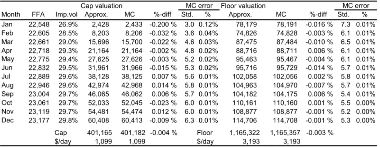
Consider the following numerical example for a calendar-year freight option with monthly settlement (j = 12). The current spot freight rate is $22,500/day, the strike price K = $25,000/day and the annualised volatility of the underlying spot freight rate is 30% (σ =0.3). In a real world pricing case we would typically use the observed FFA prices as input, but since our example is for illustrative purposes only, we simply compute FFA prices from Equation 6. We set the risk neutral freight rate drift to λ = 0.03. A positive drift for the spot price under the pricing measure implies an upward sloping term structure of forward rates. This is evident from the first column in Table 1. The constant D is calendar days. Using superscript to denote the month of the year, we have D1 = 31 (January), D2 = 28 (February), …, D12 = 31 (December). For both caps and floors we calculate the price at the start of the year for both a 7-day (panel A) and 21-day (panel B) settlement arrangement. In the first case we have T1m = 15/252 + 21*m and TNm = 21/252 + 21*m for m = 0,…,11. For the latter settlement arrangement we have T1m = 1/252 + 21*m and TNm = 21/252 + 21*m for m = 0,…,11. We assume equidistant observations (ignoring weekends and holidays) and apply Equation 11 for the plug-in variance in Equations 19 and 20. The Monte Carlo prices for each floorlet/caplet are given in the column next to the approximated price. The percentage differences between the two are also reported.
Several points are worth making about the numerical results in Table 1. First, the FFA prices in panel A are marginally higher than the corresponding prices in panel B. This is due to the fact that the settlement period in panel A starts the first trading day of the month, while in panel B it starts on day 15. Hence, all FFAs in panel A have longer time to delivery than those of panel B. Second, all floorlet prices are higher than the corresponding caplet prices as, with K > F; the floorlets are “in-the-money”. One point worth noticing is that floorlet prices do not increase monotonically with maturity (in both panel A and B); they drop in February, September and November. This is due to the “number-of-days-in-the-month” effect as the pricing formula depends on the actual number of calendar days through the constant D. The floorlet value for September is lower than August, because September has one day less than August (D9=31 versus D10=30). For February, with only 28 days, this effect is quite strong. For caplets, in our particular example, time value dominates the “number-of-days-in-the-month” effect, and therefore caplets increase monotonically with time. Finally we see that both the cap and the floor have higher prices in panel A than in panel B. There are two effects present here; different volatility inputs and different FFA prices. The first effect is the stronger. For the valuation of the caps, both effects pull in the same direction. Short delivery periods both increase the FFA prices and the variance input in panel A relative to panel B. For the floors, looking at an increase in FFA price in isolation gives higher floorlets prices in panel B than in panel A. However, an FFA with short settlement period has higher
variance than a contract with longer settlement period (cf. Equation 16) and a higher variance gives higher caplet/floorlet prices. We see from the table that the variance effect is much stronger than the price effect, resulting in a higher floor price in panel A compared to panel B.
The imp.vol column provides the volatility input that gives the same prices of a put/call in a standard Black model with maturity TN as our corresponding floorlet/caplet prices. This column demonstrates the volatility effect of the settlement period for the contracts. The underlying freight rate volatility is 30%. From Equation 13 we know that the FFAs also have 30% volatility prior to the settlement period, while it decreases to zero in the settlement period. With 30% as an upper limit for the FFA volatility we note that for the last floorlets/caplets in both panel A and panel B, volatility is very close to 30%, since the settlement period is relatively short compared to the total life of the contract. For short term contracts the definition of the settlement period has a strong effect, with implied volatility of 17.9% versus 26.9% for the contracts with settlement the following month. To sum up, Table 1 clearly shows that our analytical approximation is fairly accurate, and that the pricing error is decreasing in time to maturity.
< Insert Table 1 about here >
5. Concluding remarks
In this paper we have presented the mathematical framework for freight options modelling. Assuming lognormal spot freight dynamics, we show that FFAs are lognormal prior to the settlement period, but that this lognormality breaks down in the settlement period. We suggest approximate dynamics in the settlement period for the FFA that leads to closed form option pricing formulas for Asian call and put options written on the spot freight rate indices in the Black (1976) framework. In a Monte Carlo experiment we show that our formula gives quite accurate prices.
The analysis using implied volatility in the Black (1976) framework might be extended to a more realistic model for the underlying asset price dynamics in the Monte Carlo exercise (for example allowing for jumps and stochastic volatility). We leave this for future research.
It is also evident from maritime economic theory that other stochastic specifications of the spot (and forward) freight rate process may be more appropriate. For instance, Sødal, Koekebakker and Adland (2005) develop a real option based valuation model for combination carriers which hinges on the assumption of mean reversion of the dry bulk and tanker freight markets. Mean reversion in freight rates implies a term structure in the volatility. Future extensions of this work should incorporate the term structure of volatility that exists due to mean reversion in the spot freight rate process (cf. Koekebakker and Adland, 2004; Tvedt, 1998). The possible existence of seasonal volatility should also be investigated.
References
Adland, R., Cullinane, K., 2006. The non-linear dynamics of spot freight rates in tanker markets. Transportation Research Part E: Logistics and Transportation Review, 42(3), 211-224.
Adland, R., Cullinane, K., 2005. A time-varying risk premium in the term structure of bulk shipping freight rates. Journal of Transport Economics and Policy, 39(2), 191-208. Alziary B., Decamps, J. P., Koehl, P.F., 1997. A P.D.E approach to Asian options: analytical and numerical evidence. Journal of Banking and Finance, 21, 613-640.
Bessembinder, H., 1991. Forward contracts and firm value: investment incentive and contracting effects. Journal of Finance and Quantitative Analysis, 26, 519-532.
Bessembinder, H., Lemmon, M.L., 2002. Equilibrium pricing and optimal hedging in electricity forward markets. Journal of Finance, 57, 1347-1382.
Black, F., 1976. The pricing of commodity contracts. Journal of Financial Economics, 3, 167-179.
Black, F., Scholes, M., 1973. The pricing of options and corporate liabilities. Journal of Political Economy, 81, 637-654.
Brennan, M.J., Schwartz, E.S., 1979. A continuous time approach to the pricing of bonds. Journal of Banking and Finance, 3, 133–155.
Clewlow, L., Strickland, C., 1999. Valuing energy options in a one factor model fitted to forward price. Working paper, University of Technology, Sydney.
Clewlow, L., Strickland, C., 2000. Energy Derivatives – Pricing and Risk Management. Lacima Publications, London.
Dinwoodie, J., Morris, J., 2003. Tanker forward freight agreements: The future for freight futures? Maritime Policy and Management, 30(1), 45-58.
Dewynne, J.N., Wilmott, P., 1995. A note on average rate options with discrete sampling. SIAM Journal of Applied Mathematics, 55 (1995), 267-276.
Duffie, D., 1996. Dynamic Asset Pricing Theory. Princeton University Press, Princeton New Jersey, 2nd edition.
Froot, K., Scharfstein, D., Stein, J., 1993. Risk management: Coordinating corporate investment and financing policies. Journal of Finance, 48, 1629-1658.
Geman, H., Vasicek, O., 2001. Plugging into electricity. RISK, 14 (August), 93-97. Geman, H., Eydeland, A., 1995. Domino effect: Inverting the Laplace transform. RISK, March.
Geman, H., Yor, M., 1993. Bessel processes, Asian options and perpetuities. Mathematical Finance, 3, 349-375.
Gibson R., Schwartz, E.S., 1990. Stochastic convenience yield and the pricing of oil contingent claims. Journal of Finance, 45, 959-976.
Heath, D., Jarrow R., Morton, A., 1992. Bond pricing and the term structure of interest rates: A new methodology for contingent claim valuation. Econometrica, 60(1), 77-105. Hilliard J.E., Reis, J., 1998. Valuation of commodity futures and options under stochastic convenience yields, interest rates, and jump diffusions in the spot. Journal of Financial and Quantitative Analysis, 33(1), 61-86.
Kavussanos, M.G., Alizadeh, A., 2002. The expectations hypothesis of the term structure and risk premia in dry bulk shipping freight markets: An EGARCH-M approach. Journal of Transport Economics and Policy 36 (2), 267-304.
Kavussanos, M.G., Nomikos, N., 1999. The forward pricing function of shipping, freight futures market. Journal of Futures Markets, 19(18): 353-376.
Kavussanos, M.G., Nomikos, N., 2000a. Futures hedging when the structure of the underlying asset changes: The case of the BIFFEX contract. Journal of Futures Markets, 20(23), 775 – 801.
Kavussanos, M.G., Nomikos, N., 2000b. Dynamic hedging in the freight futures market, Journal of Derivatives, 8 (1), 40-58.
Kavussanos, M.G., Nomikos N., 2000c. Constant vs. time-varying hedge ratios and hedging efficiency in the BIFFEX market. Transportation Research Part E: Logistics and Transportation Review, 36(19), 229-248.
Kavussanos, M.G., Nomikos, N., 2003. Price discovery, causality and forecasting in the freight futures market. Review of Derivatives Research, 6(18), 203-230.
Kavussanos, M.G., Visvikis, I., 2004a. The hedging performance of over-the-counter forward shipping freight markets. In: International Association of Maritime Economists (IAME) Conference Proceedings, Izmir, Turkey, 30 June – 2 July, 2004.
Kavussanos, M.G., Visvikis, I., 2004b. Market interactions in returns and volatilities between spot and forward shipping freight markets. Journal of Banking and Finance, 28(23), 2015-2049.
Kavussanos, M.G., Visvikis, I., Batchelor, R., 2004. Over-the-counter forward contracts and spot price volatility in shipping. Transportation Research Part E: Logistics and Transportation Review, 40(19), 273-296
Kavussanos, M.G., Visvikis, I., Goulielmou, M.A., 2005. An investigation of the use of risk management and shipping derivatives: The case of Greece. In: Proceedings for the Annual Conference of the International Association of Maritime Economists (IAME), Limassol, Cyprus, June 23 – 25.
Kavussanos, M.G., Visvikis, I., Menachof, D., 2004. The unbiasedness hypothesis in the freight forward market: Evidence from cointegration tests. Review of Derivatives Research, 7(18), 241 – 266.
Kemna, A., Vorst, A., 1990. A pricing method for options based on average asset values. Journal of Banking and Finance, 14, 133-129.
Koekebakker, S., Adland, R., 2004. Modelling forward freight rate dynamics − empirical evidence from time charter rates. Maritime Policy and Management, 31(19), 319 – 335. Levy, E., 1997. Asian Options. In: Clewlow, L. and Strickland S. (Eds.) Exotic Options − The State of the Art, International Thompson Business Press, London.
Rogers, L. C. G., Shi, Z., 1995. The value of an Asian option. Journal of Applied Probability, 32, 1077-1088.
Schwartz, E.S., 1997. The stochastic behaviour of commodity prices: Implications for pricing and hedging. Journal of Finance, 52(18), 923-973.
Stulz, R., 1990. Managerial discretion and optimal financing policies. Journal of Financial Economics, 26, 3-27.
Sødal, S., Koekebakker, S., Adland, R., 2005. Market switching in shipping – a real option model applied to the valuation of combination carriers, Working Paper, Agder University College.
Taleb, N., 1997. Dynamic hedging: Managing vanilla and exotics options. Wiley, New York.
Tigkas, I., Tigka, D.. Tigkas, T., 2005. Option pricing and risk management in shipping. In: Proceedings for the SNAME Symposium on ship operations, management and economics, Athens, Greece, May 12 - 14.
Tvedt, J., 1998. Valuation of a European futures option in the BIFFEX market. Journal of Futures Markets, 18(2), 167-175.
Tvedt, J., 1997. Valuation of VLCCs under income uncertainty. Maritime Policy and Management, 24 (2), 159-174.
Vasicek O., 1977. An Equilibrium Characterisation of the Term Structure. Journal of Financial Economics, 5, 177-188.
Yor, M., 1993. From planar Brownian windings to Asian options. Insurance: Mathematics and Economics, 13, 23-34.
Zhang, J.E., 2001. A semi-analytical method for pricing and hedging continuously sampled arithmetic average rate options. Journal of Computational Finance, 5(1), 59-80.
Appendix 1 – Proofs of equations 6, 7 and 10
Proof of Equation 6: FFA price as a function of underlying spot price
Equation 6 follows from inserting Equation 5 into Equation 2 and taking expectation. The step-by-step calculation is as follows:
( )
[
]
( ) ( ) ∆ − ∆ − − − = ∆ − − = − = + − − = − − ⋅ = = = ∫ = =∑
∑
∑
∑
λ λ λ λ λ λ σ σ λ e e N e S e N e S e N S e S E N T S E N T T t F N t T t N i i t T t N i t T t N i s dW t T t Q t N i i Q t N N N i i T t Q i 1 1 1 1 ) , , ( ) ( 1 0 ) ( 1 ) ( 1 2 1 1 1 2 (A.1)This corresponds to Equation 6 in the text. The third equality follows from the expectation of a lognormal random variable, and the fourth from the assumption of equidistant observations, ∆=
(
TN −T1) (
N−1)
.Proof of Equation 7: The FFA dynamics
The dynamics for the FFA contract changes as it enters the settlement period. In particular, the volatility of the contract decreases as the settlement period gradually materialises. Therefore, the dynamics of the FFA contract must be investigated both prior to the settlement period
(
t<T1)
, and inside the settlement period(
T1<t<TN)
. First, however, we must link the FFA price to the underlying spot price.The FFA price written as a function of the underlying spot price is given by (A.1). Now assume that the first M < N fixings have already been observed so that TM < t < TM+1.
[
]
∑
∑
∑
+ = − = = + = = N M i t T t M i i N i i Q t N i e N S T S N T S E N T T t F 1 ) ( 1 1 1 ) ( 1 ) ( 1 ) , , ( λ (A.2)Now we want to apply Itó’s lemma to the expressions for the FFA prices. Itó’s lemma is a theorem of stochastic calculus that shows that second order differential terms of Wiener
processes become deterministic under stochastic integration. It is somewhat analogous to the chain rule in ordinary calculus. Let x(t)be a generalised Wiener process. That is, let
( )
,( )
, ( ) )(t a xt dt b xt dW t
dx = +
According to Itó’s lemma, f(x(t),t) is also a generalised Wiener process as follows:
(
)
( )
( )
,( )
, () 2 1 , ), ( 2 2 2 t dW x f t x b dt x f t x b t f x f t x a t t x df ∂ ∂ + ∂ ∂ + ∂ ∂ + ∂ ∂ = (A.3)Recall the dynamics of S(t) from Equation 4. To find the dynamics of F(t,T1,TN) for
(
t<T1)
, we apply Itó’s lemma to A.1. This gives
(
)
(
, ,)
( ) ) ( 1 1 1 , , 1 1 ) ( 1 ) ( 1 ) ( 1 t dW T T t F t dW e N S dt e N S e N S T T t dF N N i t T t N i t T t N i t T t N i i i σ σ λ λ λ λ λ = + − =∑
∑
∑
= − = − = − (A.4)The last equality follows from Equation A.1, and we have established the lognormal property of F(t,T1,TN) prior to T1. To find the dynamics of F(t,T1,TN) for TM < t < TM+1 with the first M < N fixings observed, apply Itó’s lemma to A.2. This gives
(
)
) ( 1 ) ( 1 1 1 , , 1 ) ( 1 ) ( 1 ) ( 1 ) ( 1 t dW e N S t dW e N S dt e N S e N S T T t dF N M i t T t N M i t T t N M i t T t N M i t T t N i i i i∑
∑
∑
∑
+ = − + = − + = − + = − = + − = λ λ λ λ σ σ λ λ (A.5)We observe from A.5 that the lognormal property no longer holds. We therefore need both A.4 and A.5 to describe the dynamics of the FFA. Dividing each of the equations A.4 and A.5 with F(t,T1,TN) proves Equation 7 in the text.
Proof of Equation 10: The volatility plug-in From Equation 8 we know that σ(t) is given by
− = + < < − ≤ = 1 , ... , 2 , 1 , 1 ) ( 1 N M M T t M T N M N T t t σ σ σ
The variance during the period
[ ]
t,TN with t<T1 is defined by ≡∫
NT t F s ds 2 2 σ( ) σ . This can be calculated explicitly as
) 6 1 2 1 3 1 ( ) ( ) ( 1 ) ( ) ( ) ( ) 1 ( ) ( ) ( ) ( ) ( ) ( ) ( 2 1 2 1 2 2 1 2 2 2 1 2 2 2 2 1 2 2 2 2 2 2 1 1 2 1 1 N N t T T T N T T N M N T T N N t T ds s ds s ds s ds s ds s N N M M T T T T T T T t T t N N M M N + − ∆ + − = − + + − − + + − − + − = + + + + + = − +
∫
∫
∫
∫
∫
− + σ σ σ σ σ σ σ σ σ σ σ L L L L (A.6)The last equality follows from the assumption of equidistant observations. This proves Equation 10 in the text.
Appendix 2 - The Monte Carlo procedure
Monte Carlo calculations are often used to check the accuracy of approximate formulas. Even though a conditional expectation cannot be solved in closed form, we can compute this expectation numerically by simulating the stochastic process at hand and computing the option price. The Monte Carlo estimate is the average option price from many simulations. The accuracy of our estimator (the difference between the Monte Carlo option price and the true option price) can be made arbitrarily small by increasing the number of simulations. We demonstrate the Monte Carlo procedure for floorlets only. In each draw, j, we simulate N prices under the martingale measure and collect the results in a vector
[
]
N
i T
T
j S S
u = ,K, . Next, we calculate the realised floorlet h(uj): + = − − − =
∑
N j j T t T r j i N S N K e u h( ) ( ) 1 1 (A.7)A simple Monte Carlo estimator fˆ for the floorlet is then ) ( 1 ˆ 1 j s j u h s f
∑
= = (A.8)when the simulation is repeated s times. The accuracy of this estimator can be expressed by the standard error
s s s σ ε = ˆ (A.9) where
− =
∑
∑
= = 2 1 2 1 2 1 ( ) 1 ( ) ˆ s j j j s j s hu s u h s σThe smaller the standard error, the closer we get to the true floorlet price. To reduce the standard deviation we have employed the control variate technique. This entails using the prices in each random draw to compute a price for a similar contract for which we do have a closed form solution.
Denote by g* the Black (1976) closed form price today for a European put option
that pays off
[
−]
+N
T
S
K at maturity TN with volatility and interest rate equal to the case of the floorlet. Define the realised put price as
[
]
+ − − − = N N T t T r j e K S u g( ) ( ) (A.10)We know that the analytical price equals the Monte Carlo price for a standard put, such that the expectation:
0 ) ( 1 1 * = −
∑
= j s j Q t g u s g E (A.11)This allows us to define a Monte Carlo estimator for the floorlet as
( )
( )
(
)
∑
= − + = s j j j g gu u h s f 1 * 1 (A.12)The standard error of this estimator can be computed the same way as before, but this estimator, with a control variate, has lower variability than the simple Monte Carlo estimate. We can see from the expression of f how variability is reduced. If an option ends out of the money, the simulated price is zero. We need more simulations just to get a positive value of our option. On the other hand, if our simulation resulted in a huge pay-off for the option, we need a lot of simulations to get the average (price) back to a reasonable level. The job of the control variate is to do this adjustment for each draw. In order for this to work satisfactorily, the actual derivative must be strongly correlated with the control variate. In our case this means that when h
( )
uj is zero, g( )
uj is typically alsozero (due to an upward drifting simulated freight rate path) leading to an upward adjustment of the price estimator in Equation A.12. Conversely, in cases where the simulated freight rate is strongly downward drifting, the adjustment is negative. Overall the adjustments cancel out due to Equation A.11. The final result is that f is less variable than fˆ , improving the efficiency of the estimator.
Figure 1: Asymptotic behaviour of an FFA price approximation. 1/6 1/3 1/2 2/3 0 2 4 6 8 10 12 14 16 18 20 22 24 26 28 30 N R(N)
Table 1: Cap and floor valuation – Closed form approximations and Monte Carlo estimates
Panel A: Settlement period last 7 trading days of each month
Cap valuation Floor valuation
Month FFA Imp.vol Approx. MC %-diff Std. % Approx. MC %-diff Std. % Jan 22,548 26.9% 2,428 2,433 -0.200 % 3.0 0.12% 78,179 78,191 -0.016 % 7.3 0.01% Feb 22,605 28.5% 8,203 8,206 -0.032 % 3.6 0.04% 74,826 74,828 -0.003 % 6.1 0.01% Mar 22,661 29.0% 15,696 15,700 -0.022 % 4.6 0.03% 87,475 87,484 -0.010 % 6.5 0.01% Apr 22,718 29.3% 21,164 21,164 -0.002 % 4.8 0.02% 88,716 88,711 0.006 % 6.1 0.01% May 22,775 29.4% 27,625 27,626 -0.003 % 5.2 0.02% 95,463 95,467 -0.004 % 6.1 0.01% Jun 22,832 29.5% 31,961 31,966 -0.015 % 5.3 0.02% 95,716 95,729 -0.014 % 5.7 0.01% Jul 22,889 29.6% 38,128 38,125 0.007 % 5.6 0.01% 102,058 102,056 0.002 % 5.8 0.01% Aug 22,946 29.6% 42,974 42,968 0.014 % 5.8 0.01% 104,963 104,970 -0.007 % 5.7 0.01% Sep 23,004 29.7% 46,065 46,062 0.006 % 5.7 0.01% 104,182 104,175 0.006 % 5.4 0.01% Oct 23,061 29.7% 52,033 52,045 -0.023 % 6.0 0.01% 110,161 110,160 0.001 % 5.5 0.00% Nov 23,119 29.7% 54,481 54,474 0.012 % 6.0 0.01% 108,877 108,877 -0.001 % 5.2 0.00% Dec 23,177 29.8% 60,408 60,413 -0.009 % 6.3 0.01% 114,706 114,708 -0.001 % 5.3 0.00% Cap 401,165 401,182 -0.004 % Floor 1,165,322 1,165,357 -0.003 % $/day 1,099 1,099 $/day 3,193 3,193
Panel B: Settlement period all 21 trading days of each month
Cap valuation Floor valuation
Month FFA Imp.vol Approx. MC %-diff Std. % Approx. MC %-diff Std. % Jan 22,529 17.9% 314 333 -5.478 % 5.7 1.72% 76,645 76,677 -0.041 % 13.0 0.02% Feb 22,586 24.7% 5,484 5,497 -0.225 % 6.7 0.12% 72,630 72,659 -0.039 % 11.2 0.02% Mar 22,642 26.6% 12,832 12,826 0.049 % 8.4 0.07% 85,190 85,192 -0.002 % 11.9 0.01% Apr 22,699 27.5% 18,586 18,588 -0.011 % 8.8 0.05% 86,699 86,708 -0.010 % 11.1 0.01% May 22,756 28.0% 25,137 25,158 -0.081 % 9.6 0.04% 93,554 93,556 -0.002 % 11.2 0.01% Jun 22,813 28.3% 29,696 29,701 -0.016 % 9.7 0.03% 94,011 94,006 0.005 % 10.6 0.01% Jul 22,870 28.6% 35,911 35,923 -0.032 % 10.4 0.03% 100,419 100,412 0.007 % 10.7 0.01% Aug 22,927 28.8% 40,863 40,861 0.005 % 10.7 0.03% 103,428 103,429 -0.001 % 10.5 0.01% Sep 22,985 28.9% 44,109 44,135 -0.060 % 10.6 0.02% 102,783 102,769 0.014 % 10.0 0.01% Oct 23,042 29.0% 50,091 50,080 0.021 % 11.2 0.02% 108,795 108,788 0.006 % 10.2 0.01% Nov 23,100 29.1% 52,668 52,653 0.027 % 11.1 0.02% 107,620 107,625 -0.004 % 9.7 0.01% Dec 23,158 29.2% 58,596 58,594 0.003 % 11.6 0.02% 113,469 113,484 -0.013 % 9.9 0.01% Cap 374,287 374,348 -0.016 % Floor 1,145,243 1,145,304 -0.005 % $/day 1,025 1,026 $/day 3,138 3,138
Assumptions: spot rate S = 22,500, market price of risk λ = 0.03, strike price K = 25,000, volatility σ = 30% Monte Carlo results are in each case based on 5,000,000 simulated spot rate paths
MC error MC error