NBER WORKING PAPER SERIES
MACRO FACTORS IN BOND RISK PREMIA Sydney C. Ludvigson
Serena Ng Working Paper 11703
http://www.nber.org/papers/w11703
NATIONAL BUREAU OF ECONOMIC RESEARCH 1050 Massachusetts Avenue
Cambridge, MA 02138 October 2005
Ludvigson acknowledges financial support from the Alfred P. Sloan Foundation and the CV Starr Center at NYU. We thank Greg Du¤ee and Monika Piazzesi for helpful comments. We are also grateful to Monika Piazzesi for help with the bond data, to Mark Watson for help with the macro data, and to Bernadino Palazzo for excellent research assistance. Any errors or omissions are the responsibility of the authors. The views expressed herein are those of the author(s) and do not necessarily reflect the views of the National Bureau of Economic Research.
©2005 by Sydney C. Ludvigson and Serena Ng. All rights reserved. Short sections of text, not to exceed two paragraphs, may be quoted without explicit permission provided that full credit, including © notice, is given to the source.
Macro Factors in Bond Risk Premia Sydney C. Ludvigson and Serena Ng NBER Working Paper No. 11703 October 2005, Revised September 2006 JEL No. G10, G12, E0, E4
ABSTRACT
Empirical evidence suggests that excess bond returns are forecastable by financial indicators such as forward spreads and yield spreads, a violation of the expectations hypothesis based on constant risk premia. But existing evidence does not tie the forecastable variation in excess bond returns to underlying macroeconomic fundamentals, as would be expected if the forecastability were attributable to time variation in risk premia. We use the methodology of dynamic factor analysis for large datasets to investigate possible empirical linkages between forecastable variation in excess bond returns and macroeconomic fundamentals. We find that several common factors estimated from a large dataset on U.S. economic activity have important forecasting power for future excess returns on U.S. government bonds. Following Cochrane and Piazzesi (2005), we also construct single predictor state variables by forming linear combinations of either five or six estimated common factors. The single state variables forecast excess bond returns at maturities from two to five years, and do so virtually as well as an unrestricted regression model that includes each common factor as a separate predictor variable. The linear combinations we form are driven by both "real" and "inflation" macro factors, in addition to financial factors, and contain important information about one year ahead excess bond returns that is not captured by forward spreads, yield spreads, or the principal components of the yield covariance matrix.
Sydney C. Ludvigson Department of Economics New York University 269 Mercer Street 7th Floor New York, NY 10003 and NBER [email protected] Serena Ng Department of Economics University of Michigan 317 Lorcha Hall Ann Arbor, MI 48109 [email protected]
1 Introduction
Recent empirical research in …nancial economics has uncovered signi…cant forecastable varia-tion in the excess returns of U.S. government bonds, a violavaria-tion of the expectavaria-tions hypothesis. Fama and Bliss (1987) report thatn-year excess bond returns are forecastable by the spread between the n-year forward rate and the one-year yield. Campbell and Shiller (1991) …nd that excess bond returns are forecastable by Treasury yield spreads. Cochrane and Piazzesi (2005) …nd that a linear combination of …ve forward spreads explains between 30 and 35 percent of the variation in next year’s excess returns on bonds with maturities ranging from two to …ve years. These …ndings imply that risk premia in bond returns and bond yields vary over time and are a quantitatively important source of ‡uctuations in the bond market.
An unanswered question is whether such movements in bond market risk premia bear any relation to the macroeconomy. Are there important cyclical ‡uctuations in bond market premia and, if so, with what macroeconomic aggregates do these premia vary? Economic theories that rationalize time-varying risk premia almost always posit that such premia vary with macroeconomic variables. For example, Campbell and Cochrane (1999) posit that risk premia on equity vary with a slow-moving habit driven by shocks to aggregate consumption. Wachter (2006) adapts the Campbell-Cochrane habit model to examine the nominal term structure of interest rates, and shows that bond risk premia (as well as equity premia) should vary with the slow-moving consumption habit. Brandt and Wang (2003) argue that risk premia are driven by shocks to in‡ation, as well as shocks to aggregate consumption. Such theories imply that rational variation in bond risk premia should be evident from forecasting regressions of excess bond returns on macroeconomic fundamentals.
Despite these theoretical insights, there is little direct evidence of a link between the macroeconomy and bond risk premia. The empirical evidence cited above, for example, …nds that excess bond returns are forecastable not by macroeconomic variables such as aggregate consumption or in‡ation, but rather by pure …nancial indicators such as forward spreads and yield spreads.
There are several possible reasons why it may be di¢ cult to uncover a direct link between macroeconomic activity and bond market risk premia. First, some macroeconomic driving variables may be latent and impossible to summarize with a few observable series. The Campbell-Cochrane habit may fall into this category. Second, macro variables are more likely than …nancial series to be imperfectly measured and less likely to correspond to the precise economic concepts provided by theoretical models. As one example, aggregate consumption is
often measured as nondurables and services expenditure, but this measure omits an important component of theoretical consumption, namely the service ‡ow from the stock of durables. Third, the models themselves are imperfect descriptions of reality and may restrict attention to a small set of variables that fail to span the information sets of …nancial market participants. This paper considers one way around these di¢ culties using the methodology of dynamic factor analysis for large datasets. Recent research on dynamic factor analysis …nds that the information in a large number of economic time series can be e¤ectively summarized by a relatively small number of estimated factors, a¤ording the opportunity to exploit a much richer information base than what has been possible in prior empirical study of bond risk premia. In this methodology, “a large number” can mean hundreds or, perhaps, even more than one thousand economic time series. By summarizing the information from a large number of series in a few estimated factors, we eliminate the arbitrary reliance on a small number of imperfectly measured indicators to proxy for macroeconomic fundamentals, and make feasible the use of a vast set of economic variables that are more likely to span the unobservable information sets of …nancial market participants.
We use dynamic factor analysis to revisit the question of whether there are important macro factors in bond risk premia. We begin with a comprehensive analysis of whether excess bond returns are predictable by macroeconomic fundamentals, and then move on to investigate whether risk premia in long-term bond yields (sometimes called term premia), vary with macroeconomic fundamentals.
Our results indicate bond premia are indeed forecastable by macroeconomic fundamen-tals, and we …nd marked countercyclical variation in bond risk premia. To implement the dynamic factor analysis methodology, we estimate common factors from a monthly panel of 132 measures of economic activity using the method of principal components. We …nd that several estimated common factors have important forecasting power for future excess returns on U.S. government bonds. Following Cochrane and Piazzesi (2005), we also construct single predictor state variables from these factors by forming linear combinations of the either …ve or six estimated common factors (denotedF5tandF6t, respectively). We …nd that such state variables forecast excess bond returns at all maturities (two to …ve years), and do so virtually as well as a regression model that includes each common factor in the linear combination as a separate predictor variable.
The magnitude of the forecastability we …nd associated with macroeconomic activity is economically signi…cant. The estimated factors have their strongest predictive power for two-year bonds, explaining 26 percent of the one two-year ahead variation in their excess returns.
But they also display strong forecasting power for excess returns on three-, four-, and …ve-year government bonds. Although this is slightly less than that found by Cochrane and Piazzesi (their single forward-rate factor, which we denote CPt, explains 31 percent of next year’s variation in the two-year bond), it is typically more than that found by Fama and Bliss (1987) and Campbell and Shiller (1991). We also …nd that our estimated factors have strong out-of-sample forecasting power for excess bond returns that is stable over time and statistically signi…cant. The factors continue to exhibit signi…cant predictive power for excess bond returns when the small sample properties of the data are taken into account.
Perhaps more signi…cantly, the estimated factors contain substantial information about future bond returns that is not contained inCPt, a variable that Cochrane and Piazzesi show subsumes the predictive content of forward spreads, yield spreads, and yield factors. For example, when both CPt and either F5t orF6t are included together as predictor variables, each variable is strongly marginally signi…cant and the regression model can explain as much as 44 percent of next year’s two-year excess bond return. This is an improvement of 13 percent over what is possible usingCPt alone.
Of all the estimated factors we study, the single most important in the linear combinations we form is a “real” factor, highly correlated with measures of real output and employment but not highly correlated with prices or …nancial variables. “In‡ation” factors, those highly correlated with measures of the aggregate price-level, also have predictive power for excess bond returns. (We discuss the interpretation of the factors further below.) Moreover, the predictable dynamics we …nd reveal signi…cant countercyclical variation in bond risk premia: excess bond returns are forecast to be high in recessions, when economic growth is slow or negative, and are forecast to be low in expansions, when the economy is growing quickly.
We emphasize two aspects of these results. First, in contrast to the existing empirical literature, (which has focused on predictive regressions using …nancial indicators), we …nd strong predictable variation in excess bond returns that is associated with macroeconomic activity. Second, the estimated factors that load heavily on macroeconomic variables have substantial predictive power for excess bond returns above and beyond that contained in the in forward spreads, yield spreads, or even yield factors estimated as the principal components of the yield covariance matrix. This behavior is ruled out by a¢ ne term structure models where the forecastability of bond returns and bond yields is completely summarized by yields or forward rates.
The …nal part of this paper investigates long-term bond yields using a simple bivariate vectorautoregression for yield spreads and the federal funds rate. The VAR errors are
or-thgonalized so that the federal funds rate does not respond contemporaneously to the yield spread innovation. We argue that movements in the term structure that are orthogonal to contemporaneous and lagged values of the federal funds rate may be interpreted as movements risk premia on long-term yields. We …nd that shocks to the yield spread holding …xed the federal funds rate have become an economically important source of variation in the short-run forecast error of the term structure over the last 20 years, but were less important in earlier periods. In the Greenspan era, these shocks are found to have a strong countercyclical component, and are forecastable by the same real factor that we …nd forecasts excess bond returns. This reinforces the conclusion from our investigation of bond returns that investors must be compensated for risks related to recessions.
When the economy is growing, these forces contribute to a ‡attening of the yield curve even in periods when the Federal Reserve has been raising interest rates. Conventional wisdom maintains that a ‡at yield curve portends a slowing of economic activity. But we …nd that shocks to the yield spread holding …xed the funds rate display no forecasting power for real activity. Accordingly, a ‡at term structure–when attributable to this component–does not portend a period of slow or negative economic growth. We show that the unusually ‡at term structure in 2004 and 2005 provides a case in point.
The rest of this paper is organized as follows. In the next section we brie‡y review related literature not discussed above. We begin with the investigation of risk premia in bond returns. Section 3 lays out the econometric framework and discusses the use of principal components analysis to estimate common factors. Here we present the results of one-year-ahead predictive regressions for excess bond returns. We also discuss an out-of-sample forecasting analysis, and a bootstrap analysis for small-sample inference. Next we explore the potential implications of our …ndings for the term structure, by studying a simple decomposition of …ve-year yield spreads. This analysis is conducted in Section 4, using a bivariate vectorautoregression. Section 5 concludes.
2 Related Literature
Our use of dynamic factor analysis is an application of statistical procedures developed else-where for the case else-where both the number of economic time series used to construct common factors, N, and the number of time periods,T, are large and converge to in…nity (Stock and Watson 2002a, 2002b; Bai and Ng 2002, 2005). Dynamic factor analysis with large N and large T is preceded by a literature studying classical factor analysis for the case where N is relatively small and …xed but T ! 1. See for example, Sargent and Sims (1977); Sargent
(1989), and Stock and Watson (1989, 1991). By contrast, Connor and Korajczyk (1986, 1988) pioneered techniques for undertaking dynamic factor analysis when T is …xed andN ! 1.
The presumption of the dynamic factor model is that the covariation among economic time series is captured by a few unobserved common factors. Stock and Watson (2002b) show that consistent estimates of the space spanned by the common factors may be constructed by principal components analysis. A large and growing body of literature has applied dynamic factor analysis in a variety of empirical settings. Stock and Watson (2002b) and Stock and Watson (2004) …nd that predictions of real economic activity and in‡ation are greatly improved relative to low-dimensional forecasting regressions when the forecasts are based on the estimated factors of large datasets. An added bene…t of this approach is that the use of common factors can provide robustness against the structural instability that plagues low-dimensional forecasting regressions (Stock and Watson (2002a)). The reason is that such instabilities may “average out” in the construction of common factors if the instability is su¢ ciently dissimilar from one series to the next. Several authors have combined dynamic factor analysis with a vector autoregressive framework to study the macroeconomic e¤ects of policy interventions or patterns of comovement in economic activity (Bernanke and Boivin (2003); Bernanke, Boivin, and Eliasz (2005), Giannone, Reichlin and Sala (2004, 2005); Stock and Watson (2005) ). Boivin and Giannoni (2005) use dynamic factor analysis of large datasets to form empirical inputs into dynamic stochastic general equilibrium models. Ludvigson and Ng (2006) use dynamic factor analysis to model the conditional mean and conditional volatility of excess stock market returns.
Our work is also related to research in asset pricing that looks for connections between bond prices and macroeconomic fundamentals. In data spanning the period 1988-2003, Pi-azzesi and Swanson (2004) …nd that the growth of nonfarm payroll employment is a strong predictor of excess returns on federal funds futures contracts. Ang and Piazzesi (2003) in-vestigate possible empirical linkages between macroeconomic variables and bond prices in a no-arbitrage factor model of the term structure of interest rates. Building o¤ of earlier work by Du¤ee (2002) and Dai and Singleton (2002), Ang and Piazzesi present a multifactor a¢ ne bond pricing model that allows for time-varying risk premia, but they allow the pricing kernel to be driven by shocks to both observed macro variables and unobserved yield factors. They …nd empirical support for this model.1 The investigation of this paper di¤ers because we
1A closely related approach is taken in recent work by Bikbov and Chernov (2005) in which the joint dynamics of yield factors, real activity, and in‡ation are explicitly modeled as part of an a¢ ne term structure model. Others, such as Kozicki and Tinsley (2001) and Kozicki and Tinsley (2005) use a¢ ne models to link the term structure to perceptions of monetary policy.
form factors from a large dataset of 132 macroeconomic indicators to conduct a model-free empirical investigation of reduced-form forecasting relations suitable for assessing more gen-erally whether bond premia are forecastable by macroeconomic fundamentals. We view our investigation as complimentary to that of Ang and Piazzesi.
3 Econometric Framework: Bond Returns
In this section we describe our econometric framework, which involves estimating common factors from a large dataset of economic activity. Such estimation is carried out using principal components analysis, a procedure that has been described and implemented elsewhere for forecasting measures of macroeconomic activity and in‡ation (e.g., Stock and Watson (2002b), Stock and Watson (2002a), Stock and Watson (2004)). Our notation for excess bond returns and yields closely follows that in Cochrane (2005). We refer the reader to those papers for a detailed description of this procedure; here we only outline how the implementation relates to our application.
Although any predictability in excess bond returns is a violation of the expectations hypothesis (where risk-premia are presumed constant), the objective of this paper is to assess whether there is palpable forecastable variation in excess bond returns speci…cally related to macroeconomic fundamentals. In addition, we ask whether macroeconomic variables have predictive power for excess bond returns above and beyond that contained in the in forward spreads, yield spreads, or yield factors estimated as the principal components of the yield covariance matrix. To examine this latter issue, we use the Cochrane and Piazzesi (2005) forward rate factor as a forecasting benchmark. Cochrane and Piazzesi have already shown that, in our sample, the predictive power of forward spreads, yield spreads, and yield factors is subsumed by their single forward-spread factor:
For t= 1; : : : T, let rx(tn+1) denote the continuously compounded (log) excess return on an
n-year discount bond in period t+ 1. Excess returns are de…ned rx(tn+1) r(t+1n) y(1)t , where
r(t+1n) is the log holding period return from buying ann-year bond at time t and selling it as ann 1year bond at time t+ 1, and yt(1) is the log yield on the one-year bond.2
A standard approach to assessing whether excess bond returns are predictable is to select a set ofK predetermined conditioning variables at timet, given by theK 1vectorZt, and
2Letp(n)
t =log price ofn-year discount bond at timet. Then the log yield is y (n)
t (1=n)p (n)
t ; and the
log holding period return isr(n)t
t+1 p (n 1) t+1 p
(n)
t :The log forward rate at timetfor loans betweent+n 1
then estimate
rx(tn+1) = 0Zt+ t+1 (1)
by least squares. For example,Zt could include the individual forward rates studied in Fama and Bliss (1987), the single forward factor studied in Cochrane and Piazzesi (2005), (a lin-ear combination of yt(1) and four forward rates), or other predictor variables based on a few macroeconomic series. For reasons discussed above, such a procedure may be restrictive, especially when investigating potential links between bond premia and macroeconomic fun-damentals. In particular, suppose we observe a T N panel of macroeconomic data with elements xit; i = 1; : : : N, t = 1; :::; T, where the cross-sectional dimension, N, is large, and possibly larger than the number of time periods, T. With standard econometric tools, it is not obvious how a researcher could use the information contained in the panel because, unless we have a way of ordering the importance of theN series in forming conditional expectations (as in an autoregression), there are potentially 2N possible combinations to consider. Fur-thermore, letting xt denote the N 1vector of panel observations at timet, estimates from the regression
rx(tn+1) = 0xt+ 0Zt+ t+1 (2)
quickly run into degrees-of-freedom problems as the dimension ofxtincreases, and estimation is not even feasible when N +K > T.
The approach we consider is to posit that xit has a factor structure taking the form
xit = 0ift+eit; (3)
where ft is a r 1 vector of latent common factors, i is a corresponding r 1 vector of latent factor loadings, and eit is a vector of idiosyncratic errors.3 The crucial point here is that r << N, so that substantial dimension reduction can be achieved by considering the regression
rx(t+1n) = 0Ft+ 0Zt+ t+1; (4)
where Ft ft. Equation (1) is nested within the factor-augmented regression, making (4) a convenient framework to assess the importance of xit via Ft, even in the presence of Zt. 3We consider anapproximate dynamic factor structure, in which the idiosyncratic errorseitare permitted to have a limited amount of cross-sectional correlation. The approximate factor speci…cation limits the contribution of the idiosyncratic covariances to the total variance ofxas N gets large:
N 1 N X i=1 N X j=1 jE(eitejt)j M; whereM is a constant.
But the distinction betweenFt andftis important, because factors that are pervasive for the panel of data xit need not be important for predicting rx
(n)
t+1.
As common factors are not observed, we replaceftbyfbt, estimates that, whenN; T ! 1, span the same space asft. (Sinceftand icannot be separately identi…ed, the factors are only identi…able up to an r r matrix.) In practice, ft are estimated by principal components analysis (PCA).4 Let the be the N r matrix de…ned as ( 01; :::; 0N)0: Intuitively, the estimated time t factors fbt are linear combinations of each element of the N 1 vector
xt= (x1t; :::; xN t)0, where the linear combination is chosen optimally to minimize the sum of squared residualsxt ft. Throughout the paper, we use “hats”to denote estimated values. To determine the composition ofFbt, we form di¤erent subsets offbt, and/or functions offbt (such asfb2
1t). For each candidate set of factors,Fbt, we regressrx
(n)
t+1 onFbtandZtand evaluate the corresponding BIC and R2. Following Stock and Watson (2002b), minimizing the BIC
yields the preferred set of factors Fbt, but we explicitly limit the number of speci…cations we search over.5 The vector Z
t contains additional (non-factor) regressors that are thought to be related to future bond returns. The …nal regression model for excess returns is based on
Zt plus this optimal Fbt. That is,
rx(t+1n) = 0Fbt+ 0Zt+ t+1: (5)
Although we have written (5) so that Fbt and Zt enter as separate regressors, there is no theoretical reason why factors that load heavily on macro variables should contain information that is entirely orthogonal to that in …nancial indicators:For this reason we are also interested in whether macro factors Fbt have unconditional predictive power for future returns. This amounts to asking whether the coe¢ cients from a restricted version of (5) given by
rx(tn+1) = 0Fbt+ t+1 (6)
are di¤erent from zero. At the same time, an interesting empirical question is whether the information contained in the estimated factors Fbt overlaps substantially with that contained 4To be precise, theT rmatrixfbispTtimes thereigenvectors corresponding to therlargest eigenvalues of theT T matrixxx0=(T N)in decreasing order. Let be theN rmatrix of factor loadings 0
1; :::; 0N 0
:
and f are not separately identi…able, so the normalization f0f =T = Ir is imposed, where Ir is the r -dimensional identity matrix. With this normalization, we can additionally obtainb =x0f =Tb , andb
it=b 0 iftb
denotes the estimated common component in series i at time t. The number of common factors, r, is determined by the panel information criteria developed in Bai and Ng (2002).
5We …rst evaluate r univariate regressions of returns on each of the r factors. Then, for only those factors that contribute signi…cantly to minimizing the BIC criterion of the r univariate regressions, we evaluate whether squared and cubed terms help reduce theBIC criterion further. We do not consider other polynomial terms, or polynomial terms of factors not important in the regressions on linear terms.
in …nancial predictor variables. Therefore we also evaluate multiple regressions of the form (5), in which Zt includes the Cochrane-Piazzesi factor CPt as a benchmark. As discussed above, we use this variable as a single summary statistic because it subsumes the information contained in a large number of popular …nancial indicators known to forecast excess bond returns. Such multiple regressions allow us to assess whether Fbt has predictive power for excess bond returns, conditional on the information in Zt: In each case, the null hypothesis is that excess bond returns are unpredictable.
Under the assumption that N; T ! 1 with pT =N !0, Bai and Ng (2005) showed that (i)(b;b)obtained from least squares estimation of (5) arepT consistent and asymptotically normal, and the asymptotic variance is such that inference can proceed as though ft is observed (i.e., that pre-estimation of the factors does not a¤ect the consistency of the second-stage parameter estimates or the regression standard errors), (ii) the estimated conditional mean,Fb0
tb+Zt0bismin[ p
N ;pT]consistent and asymptotically normal, and (iii) thehperiod forecast error from (5) is dominated in large samples by the variance of the error term, just as if ft is observed. The importance of a large N must be stressed, however, as without it, the factor space cannot be consistently estimated however large T becomes.
Although our estimates of the predictable dynamics in excess bond returns will clearly de-pend on the extracted factors and conditioning variables we use, the combination of dynamic factor analysis applied to very large datasets, along with a statistical criterion for choosing parsimonious models of relevant factors, makes our analysis less dependent than previous applications on a handful of predetermined conditioning variables. The use of dynamic factor analysis allows us to entertain a much larger set of predictor variables than what has been entertained previously, while the BIC criterion provides a means of choosing among summary factors by indicating whether these variables have important additional forecasting power for excess bond returns.
3.1 Empirical Implementation and Data
A detailed description of the data and our sources is given in the Data Appendix. We study monthly data spanning the period 1964:1 to 2003:12, the same sample studied by Cochrane and Piazzesi (2005).
The bond return data are taken from the Fama-Bliss dataset available from the Center for Research in Securities Prices (CRSP), and contain observations on one- through …ve-year zero coupon U.S. Treasury bond prices. These are used to construct data on excess bond returns, yields and forward rates, as described above. Annual returns are constructed by
continuously compounding monthly return observations.
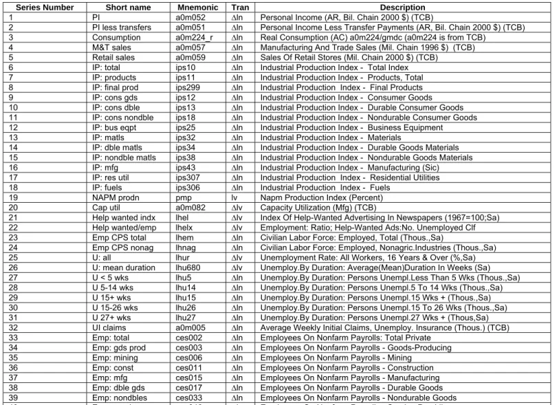
We estimate factors from a balanced panel of 132 monthly economic series, each spanning the period 1964:1 to 2003:12. Following Stock and Watson (2002b, 2004, 2005), the series were selected to represent broad categories of macroeconomic time series: real output and income, employment and hours, real retail, manufacturing and sales data, international trade, consumer spending, housing starts, inventories and inventory sales ratios, orders and un…lled orders, compensation and labor costs, capacity utilization measures, price indexes, interest rates and interest rate spreads, stock market indicators and foreign exchange measures. The complete list of series is given in the Appendix, where a coding system indicates how the data were transformed so as to insure stationarity. All of the raw data inxtare standardized prior to estimation.
Notice that the estimated factors we study will not be pure macro variables, since the panel of economic indicators from which they are estimated contain …nancial variables as well as macro variables. Theoretically speaking, there is no reason why …nancial and macro variables shouldn’t be informative, since the two classes of variables must be endogenously determined by a common set of primitives. The important point, made below, is that several of the estimated factors that are highly correlated with macroeconomic activity (but little correlated with …nancial indicators) contain economically important predictive power for bond returns that is not contained in …nancial indicators with known forecasting power for bond returns, e.g., bond yields and forward rates.
For the speci…cations in which we include additional predictor variables in Zt; we report results in whichZt contains the single variableCPt. We do so because the Cochrane-Piazzesi factor summarizes virtually all the information in individual yield spreads and forward spread that had been the focus of prior work on predictability in bond returns. We also experimented with including the dividend yield on the Standard and Poor composite stock market index inZt, since Fama and French (1989) …nd that this variable has modest forecasting power for bond returns. We do not report those results, however, since the dividend yield has little forecasting power for future bond returns in our sample and has even less once the estimated factors Fbt or the Cochrane and Piazzesi factor are included in the forecasting regression.
In estimating the time-t common factors, we face a decision over how much of the time-series dimension of the panel to use. We take two approaches. First, we run in-sample regressions in which the full sample of time-series information is used to estimate the common factors at each date t. This approach can be thought of as providing smoothed estimates of the latent factors,ft. Smoothed estimates of the latent factors are the most e¢ cient means of
summarizing the covariation in the data x because the estimates do not discard information in the sample. Second, we conduct an out-of-sample forecasting investigation in which the predictor factors are reestimated recursively each period using data only up to time t. A description of this procedure is given below.
3.2 Empirical Results
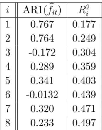
Table 1 presents summary statistics for our estimated factorsfbt: The number of factors,r, is determined by the information criteria developed in Bai and Ng (2002). The criteria indicate that the factor structure is well described by eight common factors. The …rst factor explains the largest fraction of the total variation in the panel of data x, where total variation is measured as the sum of the variances of the individual xit. The second factor explains the largest fraction of variation in x, controlling for the …rst factor, and so on. The estimated factors are mutually orthogonal by construction. Table 1 reports the fraction of variation in the data explained by factors 1 toi.6 Table 1 shows that a small number of factors account for
a large fraction of the variance in the panel dataset we explore. The …rst …ve common factors of the macro dataset account for about 40 percent of the variation in the macroeconomic series.
To get an idea of the persistence of the estimated factors, Table 1 also displays the …rst-order autoregressive, AR(1), coe¢ cient for each factor. None of the factors have a persistence greater than 0.77, but there is considerable heterogeneity across estimated factors, with coe¢ cients ranging from -0.17, to 0.77.
As mentioned, we formally choose among a range of possible speci…cations for the forecast-ing regressions of excess bond returns based on the estimated common factors (and possibly nonlinear functions of those factors such as fb3
1t) using the BIC criterion, (though we restrict our speci…cation search as described above.) We report results only for the speci…cations analyzed that have the lowest BIC criterion.7 Results not reported indicate that, when the
Cochrane-Piazzesi factor is excluded as a predictor, the six-factor subset Ft ft given by
Ft = F!6t = Fb1t;Fb13t;Fb2t;Fb3t;Fb4t;Fb8t
0
minimizes the BIC criterion across a range of pos-sible speci…cations based on the …rst eight common factors of our panel dataset, as well as nonlinear functions of these factors. Fb3
1t; above, denotes the cubic function in the …rst esti-6This is given as the the sum of the …rstilargest eigenvalues of the matrixxx0 divided by the sum of all
eigenvalues.
7Speci…cations that include lagged values of the factors beyond the …rst were also examined, but additional lags were found to contain little information for future returns that was not already contained in the one-period lag speci…cations.
mated factor. The estimated factors Fb5t and Fb6t exhibit little forecasting power for excess bond returns. When CPt is included, by contrast, the …ve-factor subset Ft ft given by
Ft = F!5t = Fb1t;Fb13t;Fb3t;Fb4t;Fb8t
0
minimizes the BIC criterion. As we shall see, the sec-ond estimated factor Fb2t is highly correlated with interest rates spreads. As a result, the information it contains about future bond premia is subsumed in CPt.
The subsetsFtcontain …ve or six factors. To assess whether a single linear combination of these factors forecasts excess bond returns at all maturities, we follow Cochrane and Piazzesi (2005) and form single predictor factors as the …tted values from a regression of average (across maturity) excess returns on the set of six and …ve factors, respectively. We denote these single factors F6t and F5t, respectively:
1 4 5 X n=2 rx(t+1n) = 0+ 1Fb1t+ 2Fb13t+ 3Fb2t+ 4Fb3t+ 5Fb4t+ 6Fb8t+ut+1; (7) F6t b0F!6t; 1 4 5 X n=2 rx(t+1n) = 0 + 1Fb1t+ 2Fb13t+ 3Fb3t+ 4Fb4t+ 5Fb8t+vt+1; (8) F5t b 0 ! F5t;
where b andbdenote the 6 1 and 5 1vectors of estimated coe¢ cients from (7) and (8), respectively. With these factors in hand, we now turn to an empirical investigation of their forecasting properties for excess bond returns.
3.2.1 In-Sample Analysis
Tables 2a-2d present results from in-sample forecasting regressions of the general form (5), for two-year, three-, four-, and …ve-year log excess bond returns.8 In this section, we in-vestigate the two hypotheses discussed above. First we ask whether the estimated factors have unconditional predictive power for excess bond returns; this amounts to estimating the restricted version of (5) given in (6), where 0 is restricted to zero. Next we ask whether the estimated factors have predictive power for excess bond returns conditional on Zt. This amounts to estimating the unrestricted regression (5) with 0 freely estimated. The statistical signi…cance of the factors is assessed using asymptotic standard errors. Section 5.3, below, investigates the …nite sample properties of the data.
For each regression, the regression coe¢ cients, heteroskedasticity and serial-correlation robust t-statistics, and adjusted R2 statistic are reported. The asymptotic standard errors
use the Newey and West (1987) correction for serial correlation with 18 lags. The correction is needed because the continuously compounded annual return has an MA(12) error structure under the null hypothesis that one-period returns are unpredictable. Because the Newey-West correction down-weights higher order autocorrelations, we follow Cochrane and Piazzesi (2005) and use an 18 lag correction to better insure that the procedure fully corrects for the MA(12) error structure.
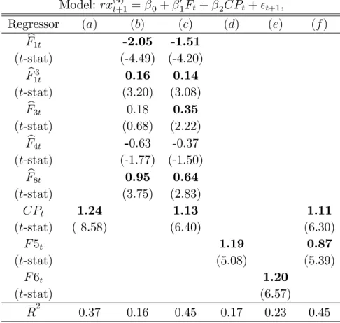
We begin with the results in Table 2a, predictive regressions for excess returns on two-year bonds rx(2)t+1. As a benchmark, column a reports the results from a speci…cation that includes only the Cochrane-Piazzesi factorCPtas a predictor variable. This variable, a linear combination ofyt(1) and four forward rates,g(2)t ; g(3)t ; :::; gt(5), is strongly statistically signi…cant and explains 31 percent of next year’s two-year excess bond return. By comparison, column
b shows that the six factors contained in the vector F!6t are also strong predictors of the two-year excess return, with t-statistics in excess of …ve for the …rst estimated factor Fb1t, but with all factors statistically signi…cant at the 5 percent or better level. Together these factors explain 26 percent of the variation in one year ahead returns. Although the second factor, Fb2t, is strongly statistically signi…cant in column b, columnc shows that once CPt is included in the regression, it loses its marginal predictive power and the adjustedR2 statistic rises from 26 to 45 percent. The information contained in Fb2t is more than captured byCPt. Because we …nd similar results for the excess returns on bonds of all maturities, we hereafter omit output from multivariate regressions usingFb2t and CPt as a separate predictors.
Columnsd throughh display estimates of the marginal predictive power of the estimated factors in F!5t and the single predictor factors F5t and F6t. The single predictor factors explain virtually the same fraction of future excess returns as do the unrestricted speci…cations that include each factor as separate predictor variables. For example, both F!6t and F6t explain 26 percent of next year’s excess bond return; both F!5t and F5t explain 22 percent. Column e shows that the …ve factors in F!5t are strongly statistically signi…cant even when
CPt is included, implying that these factors contain information about future returns that is not contained in forward spreads. The 45 percent R2 from this regression indicates an economically large degree of predictability of future bond returns. About the same degree of predictability is found when the single factorF5t is included with CPt (R
2
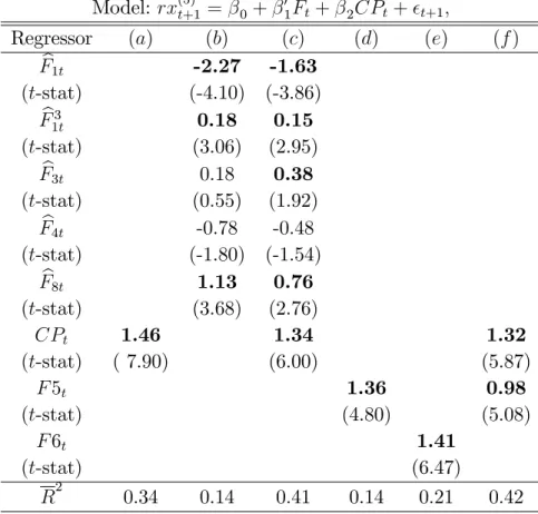
= 44 percent). The results in Tables 2b-2d for excess returns on three-, four-, and …ve-year bonds are similar to those reported in Table 2a for two-year bonds. In particular, (i) the single factors
F5t and F6t predict future bond returns just as well than the unrestricted regressions that include each factor as separate predictor variables, (ii) the …rst estimated factor continues to
display strongly statistically signi…cant predictive power for bonds of all maturities, and (iii) the speci…cations explain an economically large fraction of the variation in future returns. There are, however, a few notable di¤erences from Table 2a. The coe¢ cients on the third and fourth common factors are more imprecisely estimated in unrestricted regressions of rx(3)t+1,
rx(5)t+1, and rx(5)t+1 on F!5t, as evident from the lower t-statistics. But notice that, in every case, the third factor retains the strong predictive power it exhibited for rx(2)t+1 once CPt is included as an additional predictor (column c of Tables 2b-2d). Moreover, the single factors
F5t andF6t remain strongly statistically signi…cant predictors of excess returns on bonds of all maturities and continue to deliver high R2. F6t alone explains 24, 23, and 21 percent of next years excess return on the three-, four-, and …ve-year bond, respectively; F5t explains 19, 17, and 14 percent of next years excess returns on these bonds, andF5tandCPttogether explain 44, 45, and 42 percent of next years excess returns. When the information in CPt and Fbt is combined, the magnitude of forecastability exhibited by excess bond returns is remarkable.
Implications for A¢ ne Models The results reported in Tables 2a-2b indicate that good forecasts of excess bond returns can be made with only a few estimated factors, and that the best forecasts are based on combinations of factors that summarize information from a large panel of economic activity and the Cochrane-Piazzesi factor CPt. It is reassuring that some of estimated factors (Fb2t in particular, and to a lesser extent Fb3t) are found to contain information that is common to that the Cochrane-Piazzesi factor, suggesting that
CPt summarizes a large body of information about economic and …nancial activity.
The crucial point, however, is that measures of real activity and in‡ation in the aggregate economy contain economically meaningful information about future bond returns that is not contained in CPt, and therefore not contained in forward spreads, yield spreads, or even yield factors estimated as the principal components of the yield covariance matrix. (The …rst three principal components of the yield covariance matrix are the “level,” “slope,” and “curvature,” yield factors studied in term structure models in …nance.) These …ndings are ruled out by a¢ ne term structure models where the forecastability of bond returns and bond yields is completely summarized by yields or forward rates. In a¢ ne models, log bond prices are linear functions of the state variables. Thus, if there are K state variables, bond yields can serve as state variables, and will contain any forecasting information that is in the state variables. Since bond returns, forward rates, and yields are all linear functions of one another, a¢ ne models imply that any of these variables should contain all the forecastable information
about future bond returns and yields.9 Thus the …ndings reported above suggest that a¢ ne
models may fail to describe an important aspect of bond data.
Economic Interpretation of the Factors What economic interpretation can we give to the predictor factors? Because the factors are only identi…able up to ar rmatrix, a detailed interpretation of the individual factors would be inappropriate. Nonetheless, it is useful to brie‡y characterize the factors as they relate to the underlying variables in our panel dataset. Figures 1 through 5 show the marginalR2 for our estimates ofF1t,F2t,F3t,F4t, andF8t. The marginal R2 is the R2 statistic from regressions of each of the 132 individual series in our panel dataset onto each estimated factor, one at a time, using the full sample of data. The …gures display theR2 statistics as bar charts, with one …gure for each factor. The individual
series that make up the panel dataset are grouped by broad category and labeled using the numbered ordering given in the Data Appendix.
Figure 1 shows that the …rst factor loads heavily on measures of employment and produc-tion (employees on nonfarm payrolls and manufacturing output, for example), but also on measures of capacity utilization and new manufacturing orders. It displays little correlation with prices or …nancial variables. We call this factor a real factor. The second factor, which has a correlation with CPt of -45%, loads heavily on several interest rate spreads (Figure 2), explaining almost 70 percent of the variation in the Baa Fed funds rate spread. The third and fourth factors load most heavily on measures of in‡ation and price pressure but display little relation to employment and output. Figure 3 and 4 show that they are highly correlated with both commodity prices and consumer prices, whileFb4tis also highly correlated with the level of nominal interest rates (for example by the …ve-year government bond yield). Nominal interest rates may contain information about in‡ationary expectations that is not contained in measures of the price level. We call both Fb3t and Fb4t in‡ation factors.
Finally, Figure 5 shows that the eighth estimated factor, Fb8t, loads heavily on measures of the aggregate stock market. It is highly correlated with the log di¤erence in both the composite and industrial Standard and Poor’s Index and the Standard and Poor’s dividend yield but bears little relation to other variables. We call this factor a stock market factor. It should be noted, however, that this factor is not merely proxying for the stock market dividend yield, shown elsewhere to have predictive power for excess bond returns (e.g., Fama and French (1989)). The factor’s correlation with the dividend yield is less than 60% in our sample (Figure 5). Moreover, results not reported indicate that–conditional on the dividend
yield–the stock market factor we estimate displays strong marginal predictive power for future excess returns.
Since the factors are orthogonal by construction, we can characterize their relative impor-tance inF5t and F6t by investigating the absolute value of the coe¢ cients on each factor in the regressions (7) and (8). (Since the factors are identi…able up to anr rmatrix, the signs of the coe¢ cients have no particular interpretation.) Because the factors are orthogonal, it is su¢ cient for this characterization to investigate just the coe¢ cients from the regression on all six factors contained in F!6t, as in (7).10 Using data from 1964:1-2003:12, we …nd the following regression results (t-statistics in parentheses):
1 4 5 X n=2 rx(t+1n) = 1:03 (2:96) ( 51:72:12) b F1t+ 0:13 (2:97) b F13t 1:01 ( 3:90) b F2t+ 0:18 (1:18) b F3t 0:56 ( 2:40) b F4t+ 0:78 (4:56) b F8t+ut+1; R2 = 0:224:
The real factor, Fb1t, has the largest coe¢ cient in absolute value, implying that it is the single most important factor in the linear combinations we form. The interest rate factor
b
F2t is second most important, and the stock market factor Fb8t third most. The in‡ation factors Fb3t and Fb4t are relatively less important but still contribute more than the cubic in the real factor. (Fb3t is not marginally signi…cant in these regressions because its coe¢ cient is imprecisely estimated in forecasts of three-, four-, and …ve-year excess bond returns when only factors are included as predictors. The variable is nonetheless an important predictor of future bond returns because it is a strongly statistically signi…cant once CPt is included as an additional regressor.) It is also worth noting that Fb1t and Fb13t account for half of the adjusted R-squared statistic reported above.
In most empirical applications involving macro variables, researchers choose a few time series thought to be representative of aggregate activity. In monthly data, the usual suspects tend to be a measure of industrial production, consumer and commodity in‡ation, and un-employment. The next regression shows what happens if individual series of this type are used to forecast excess bond returns:
1 4 5 X n=2 rx(t+1n) = 6:06 (2:88) ( 028::0174) IPt+ 0(0::5602) CP It ( 20:09:55) CM P It ( 011::8079) P P It+ 1(0::3699) U Nt+ut+1; R2 = 0:113: 10Strictly speaking,Fb3
IPt is the log di¤erence in the industrial production index, CP It is the log di¤erence in the consumer price index,CM P Itis the log di¤erence in the NAPM commodity price index;P P It is the log di¤erence in the producer price index, and U Nt is the unemployment rate for the total population over 16 years of age. Unlike the factors, many of the usual suspect macro series have little marginal predictive power for excess bond returns, and the R2 statistic is lower. Interestingly, this occurs even though, for example, IPt and Fb1t have a simple correlation of 83 percent in our sample. Of course, the choice of predictors above is somewhat arbitrary given the large number of series available, and it is surely the case that di¤erent speci…cations would lead to di¤erent results. (The cubic inIPt, however, is not a statistically important predictor.) This fact serves to illustrate a point: when the information from hundreds of predictors is systematically summarized, the possibility of omitting relevant information is much reduced.
Are Bond Risk Premia Countercyclical? The …ndings presented so far indicate that excess bond returns are forecastable by macroeconomic aggregates, but they do not tell us whether there is a countercyclical component in risk premia, as predicted by economic theory. To address this question, Figure 6 plots the 12 month moving average of bothFb1tandIPtover time, along with shaded bars indicating dates designated by the National Bureau of Economic Research (NBER) as recession periods. The …gure shows that the real factor, Fb1t, captures marked cyclical variation in real activity. The correlation between the moving averages of the two series plotted is 92 percent. Both Fb1t and IP growth reach peaks in the mid-to-late stages of economic expansions, and take on their lowest values at the end of recessions. Thus recessions are characterized by low (typically negative) IP growth and low values for Fb1t, while expansions are characterized by strong positive IP growth and high values for Fb1t.
Connecting these …ndings back to the forecasts of excess bond returns, we see that excess return forecasts are high whenFb1tislow (Table 2). These …ndings imply that return forecasts have a countercyclical component, consistent with economic theories in which investors must be compensated for bearing risks related to recessions. For example, Campbell and Cochrane (1999) and Wachter (2006) study models in which risk aversion varies over the business cycle and is low in good times when the economy is growing quickly. In these models, risk premia (excess return forecasts) are low in booms but high in recessions, consistent with what we …nd. The evidence that in‡ation factors also govern part of the predictable variation in excess bond returns is consistent with economic theories for which risk premia vary with in‡ation (e.g., Brandt and Wang (2003)), as well as with theories for which in‡ation and real activity
contribute signi…cantly to variation in the price of risk (e.g.,Ang and Piazzesi (2003)). 3.2.2 Out-of-Sample Analysis and Small Sample Inference
We have formed the factors and conducted the regression analysis using the full sample of data. In this section we report results on the out-of-sample forecasting performance of the regression models studied in the previous section.11 This procedure involves fully recursive
factor estimation and parameter estimation using data only through time t for forecasting at time t+ 1. We conduct two model comparisons. First, we compare the out-of-sample forecasting performance of the …ve-factor model that includes the estimated factors in F!5t to a constant expected returns benchmark where, apart from an MA(12) error term, excess returns are unforecastable as in the expectations hypothesis.12 Second, we compare the out-of-sample forecasting performance of a speci…cation that includes the same …ve macro factors plus to the Cochrane-Piazzesi factor, CPt, to a benchmark model that includes just the Cochrane-Piazzesi factor, CPt, and a constant. This second speci…cation allows us to assess the incremental predictive power of the macro factors above and beyond the predictive power inCPt:
Table 3 reports results from one year ahead out-of-sample forecast comparisons of log excess bond returns, rx(t+1n); n = 2; ::;5. For each forecast, M SEu denotes the mean-squared forecasting error of the unrestricted model including predictor factors F!5t or F!5t and CPt;
M SEr denotes the mean-squared forecasting error of the restricted benchmark (null) model that excludes additional forecasting variables. In the column labeled “M SEu=M SEr”, a number less than one indicates that the model with the predictor factors F!5t or F!5t and
CPt has lower forecast error than the benchmark model that excludes additional predictor variables.
Results for two forecast samples are reported: 1985:1-2003:2; 1995:1-2003:2. The re-sults for the …rst forecast sample are reported in Rows 1, 3, 5, and 7 for rx(2)t+1, ...,rx(5)t+1
respectively. Here the parameters and factors were estimated recursively, with the initial estimation period using only data available from 1964:12 through 1984:12. Next, the fore-casting regressions were run over the periodt =1964:12,...,1984:12 (dependent variable from 11An important caveat with out-of-sample statistical tests is that they lack power relative to in-sample regression forecasts (Inoue and Kilian (2004)). With this caveat in mind, we proceed using tests known to have the best size and power properties among those available (Clark and McCracken (2001)).
12Notice that this procedure is conservative, since the out-of-sample performance of the estimated factors could only stronger if, in each recursion, we conducted a BIC speci…cation search to select the subset of factors with the highest predictive power. But a recursive speci…cation search would tell us nothing about the out-of-sample performance of the factors investigated above, so we do not pursue that avenue here.
t=1965:1,...,1984:12, independent variables fromt =1964:1,...,1983:12) and the estimated pa-rameters and values of the regressors at t =1984:12 were used to forecast annual compound returns for 1985:12.13 All parameters and factors are then reestimated from 1964:1 through
1985:1, and forecasts were recomputed for excess returns in 1986:1, and so on, until the …nal out-of-sample forecast is made for returns in 2003:12:The same procedure is used to compute results reported in the other rows, where the initial estimation period is t=1964:1,...,1995:1. The column labeled “Test Statistic”in Table 3 reports the ENC-NEW test statistic of Clark and McCracken (2001) for the null hypothesis that the benchmark model encompasses the unrestricted model with additional predictors. The alternative is that the unrestricted model contains information that could be used to improve the benchmark model’s forecast. “95% Asympt. CV”gives the 95th percentile of the asymptotic distribution of the ENC-NEW test statistic.
The results show that the model including the …ve factors in F!5t improves substantially over the constant expected returns benchmark, for excess bond returns of every maturity. The models have a mean-squared error that is anywhere from 79 to 93 percent of the con-stant expected returns benchmark mean-squared error, depending on the excess return being forecast and the forecast period. For the period 1995:1-2003:12 the model has a forecast error variance that is only 84, 86, 89, and 93 percent of the constant expected returns benchmark for rx(2)t+1, ...,rx(5)t+1 respectively. The ENC-NEW test statistic always indicates that the im-provement in forecast power is strongly statistically signi…cant, at the one percent or better level. Moreover, the reduction in mean-square-error over the benchmark is about the same regardless of which forecast period is analyzed.
The results also show that the model including the …ve factors in F!5t and CPt improves substantially over a benchmark that includes a constant and CPt. This reinforces the con-clusion form the in-sample analysis, namely that the estimated factors contain information about future returns that is not contained in theCP factor. The models that include the …ve factors in addition to theCP factor have a mean-squared error that is any where from 81 to 94 percent of that of the benchmark that includes only CP and a constant. The ENC-NEW test statistic always indicates that the improvement in forecast power is strongly statistically signi…cant, at the one percent or better level.
To guard against inadequacy of the asymptotic approximation in …nite samples, the Ap-pendix reports the results of a comprehensive bootstrap inference for speci…cations using four 13Note that the regressors must be lagged 12 months to account for the 12-period overlap induced from continuously compounding monthly returns to obtain annual returns.
regression models. The results show that the magnitude of predictability found in historical data is too large to be accounted for by sampling error in samples of the size we currently have. The statistical relation of the factors to future returns is evident, even accounting for the small sample distribution of standard test statistics.
4 A Decomposition of Yield Spreads
The evidence above suggests that risk premia on bond returns vary signi…cantly with real activity, as captured byFb1t. Researchers in macroeconomics are often more interested in the behavior of bondyields rather than returns. The aim of this section is to investigate whether movements in yield risk premia are also related to real economic activity, in a manner similar to that documented above for return risk premia.
It is not a given that they should be so related. While there is a simple linear relation between returns and yields, there is no simple linear transformation between their risk pre-mium components. To see this, note that then-period yield can be written as the average of expected future nominal short-rates plus an additional term (tn), which we refer to as a yield risk-premium: yt(n) = 1 NEt y (1) t +y (1) t+1+ +y (1) t+N 1 + (n) t : (9)
In the expectations hypothesis, the yield risk premium, (tn), is assumed constant.
We refer to the yield risk premium (tn) interchangeably as a term premium. The term premium should not be confused with the term spread itself, which is simply the di¤erence in yields between the n-period bond and the one-period bond. Of course, without restrictions of some kind on (tn), the equation above is just a statement of yields, not a model. But with
(n)
t constant, as in the expectations hypothesis, excess bond returns (studied above) should be unforecastable. Thus the evidence above implies that risk premia in yields, (tn), also vary. The precise relation between term premia and risk premia is likely to be complicated and nonlinear, however, because the latter is a function of the expected one-period change in the risk premium on yields, (tn) Et
(n 1)
t+1 ;which in principle varies both with maturity and over
time. It therefore remains an open question as to whether term premia are closely related to the same empirical state variables that return risk premia are found to be in linear forecasting regressions.
In this section we …rst identify movements in the term structure that are plausibly related to the risk-premium component, (tn), and then ask how movements in (tn) are related toFb1t. To accomplish the …rst objective, we decompose the term structure using a simple bivariate
vectorautoregression (VAR) for the yield spread and the federal funds rate. The VAR errors are orthgonalized so that the federal funds rate does not respond contemporaneously to the yield spread innovation. Using this orthogonalization, innovations in the yield spread will be orthogonal to contemporaneous and lagged values of the federal funds rate,F Ft.
It is natural to interpret these orthogonalized innovations as movements in risk premia,
(n)
t . For example, the expectation term above, a function of future nominal rates, captures movements in expected in‡ation and expected real interest rates. If the Federal Reserve cares only about in‡ation and the output gap, it will move the funds rate in response to anticipated changes in these variables, but it will not react to ‡uctuations in the yield curve that are orthogonal to expected in‡ation and expected real interest rates, (which a¤ect the output gap). Thus, if the yield curve changes but the federal funds rate does not, that must signify a movement in risk premia. We use this interpretation of Federal Reserve behavior as an identi…cation assumption.
In practice, the Federal Reserve is known to move gradually in response to changes in expected in‡ation and expected real interest rates. Moreover, the bond market may move in anticipation of policy changes by the Federal Reserve. Nevertheless, the funds rate, as the target of the monetary authority, summarizes a large amount of economic information upon which expectations of future in‡ation and future real interest rates are based; it is also extremely persistent. Given these facts, we assume that current and lagged values of the fed-eral funds rate (included in the VAR), summarize the market’s expectations of future Fedfed-eral Reserve policy, so that the VAR innovations in the yield spread equation (orthogonalized as described above) capture genuine movements in risk premia.14 Thus we label the residual
in the yield spread equation a “risk premium” component, and present evidence below on this identi…cation assumption. However one labels this component, we argue that it is of interest in its own right, as discussed below. We use the terms “orthogonalized yield spread innovation” and “risk premium component” interchangeably to describe this VAR residual.
Two features of this VAR decomposition deserve emphasis. First, the decomposition is intended to isolate movements in the term structure that may be plausibly related to move-14Some researchers have used federal funds futures rates to measure the …nancial market’s expectation of future federal funds rates changes (Krueger and Kuttner (1996), Rudebusch (1998), Brunner (2000), Kuttner (2001), Bernanke and Kuttner (2003)). There are at least two drawbacks with this approach for our application. First, the data from the futures market is more limited, which restricts the sample size. Second, and more important for our application, Piazzesi and Swanson (2004) show that a signi…cant fraction of the variation in feds funds futures re‡ects movements in risk-premia, not merely movements in expected future funds rates. Since we are interested in the risk premium component of yields, we do not include federal funds futures data in our VAR.
ments in risk premia; it is not intended to fully characterize the term premium component of yield spreads. To see this, observe that any movement in term premia that is correlated with the funds rate (and therefore expected future short rates) would not be captured by our or-thogonalized decomoposition. Second, we do not assign any interpretation to the innovations in the federal funds equation. In particular, we do not consider them policy shocks or even exogenous movements in the funds rate. The aim is to use the bivariate VAR to decompose yields in an interesting way, not to identify policy shocks.
Such a decomposition would be made more di¢ cult by estimating a larger VAR (as would be required to identify policy shocks). Under the identifying assumption given above, any movement in the yield spread associated with funds rate changes is correlated with the expectations component in (9). All remaining movements (given by the orthogonalized VAR residuals), must re‡ect movements in risk-premia (tn). Including additional variables in the VAR would hamper this identi…cation, since the residuals in the yield spread equation would then be orthogonal not only to the funds rate itself, but also to movements in the additional variables holding …xed the funds rate. Under our identi…cation assumption, these latter movements in the term structure reveal movements in risk premia. Since these are precisely the movements we seek to identify as part of the residual, it is important not to remove them by estimating a larger VAR. The essence of our identi…cation assumption is that the federal funds rate itself summarizes a large amount of economic information upon which expectations are based, so it is not necessary to include this information along with the funds rate in the VAR.
The procedure just described decomposes movements in the term structure; it does not provide a complete statistical model of yield changes. It is more common in the term structure literature to measure movements in yield risk premia by imposing multifactor a¢ ne models that prohibit arbitrage. The “model”in our decomposition approach boils down to assump-tions about Federal Reserve behavior that may admittedly be di¢ cult to assess empirically. On the other hand, the approach allows us to sidestep the counterfactual implication of a¢ ne term structure models that bond yields should completely drive out macroeconomic variables as interest rate and return forecasters. This latter consideration is important for our appli-cation, since the results above imply that risk premia in returns move with real economic activity unrelated to yields, forward rates and lagged returns.
We focus on the spread between the …ve-year Treasury bond and the one-year bond using quarterly data, available from the Federal Reserve. We use quarterly data in order to insure that each observation in our sample contains a meeting of the Federal Open Market
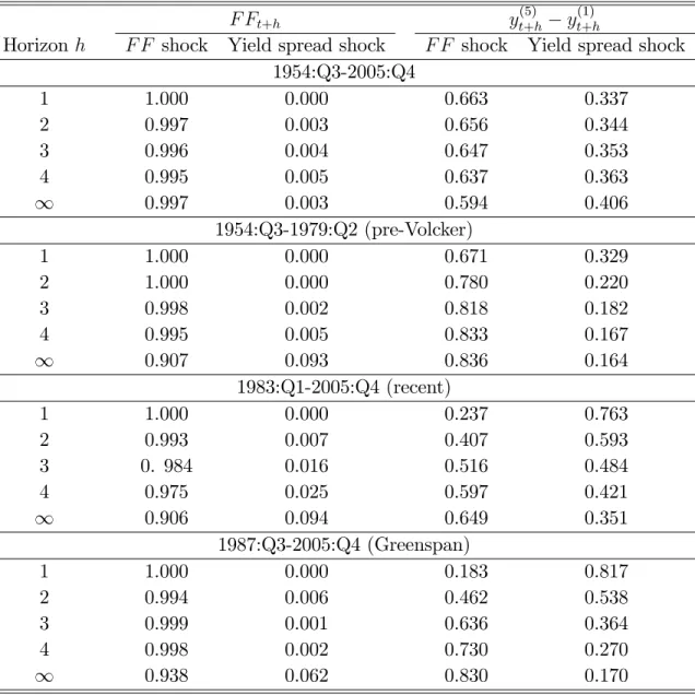
Commit-tee, at which the Federal Reserve sets interest rates. Table 4 plots variance decompositions from a two-lag, bivariate VAR for the funds rate and the …ve-year Treasury yield spread,
y(5)t y(1)t . Below, we denote the orthgonalized VAR residual in the yield spread, ry(5 1)t :
Several points about the variance decompositions bear noting.
First, in the full sample, yield spread innovations have a negligible a¤ect on the funds rate but an economically signi…cant a¤ect on yields. The innovations explain 34 percent of the one-step-ahead forecast error in the …ve-year yield spread, and roughly 40 percent of the overall variation in the yield spread. Thus, shocks to the yield curve holding …xed the funds rate account for a large fraction of the variance in the term spread in our sample.
Second, yield spread innovations have become more important over time. We study this decomposition over three subperiods: 1964:Q1-1979:Q2 (pre-Volcker), 1983:Q1-2005:Q4 (re-cent) and 1987:Q3-2005:Q4 (Greenspan). (We omit the interim years from 1979 to 1983, in which the Federal Reserve was experimenting with a nonborrowed reserve operating proce-dure.) Comparing the early period to the two latter periods, we see that fraction of forecast error variance in the yield spread that is explained by its own shocks has risen dramatically, especially in the short-run. For example, in the Greenspan period, this component explains the vast majority–82 percent–of the one-step ahead forecast error in the yield spread. The results are similar for the “recent period.”Yield spread innovations explain 76 percent of the one-step-ahead forecast error in yields and 35 percent over long horizons. By contrast, in the pre-Volcker period, yield spread innovations explain only 33 percent of one-step-ahead fore-cast error in yields and 16 percent over long horizons. These …ndings imply that movements in the term structure that are orthogonal to movements in the funds rate have become a much more economically important source of variation in yields in recent decades.
Third, the di¤erences in variance decompositions across subperiods appear more attribut-able to di¤erences in the volatility of the orthogonalized forecast errors across subperiods than to di¤erences in the VAR parameter estimates. Indeed, Figure 9 shows that the impulse responses to a one-standard deviation increase in the yield spread are quite similar across subperiods. Moreover, if we …x the VAR parameters at their full sample estimated values, we …nd a large increase in the standard deviation of the orthogonalized yield spread residual in the recent sample compared to the pre-Volcker sample. This standard deviation is normalized to one in the full sample, but is 0.76 in the pre-Volcker sample and 1.11 in the recent sample. (This can be seen clearly in Figure 10, discussed below.) We conclude that it is reasonable to use the full sample to form a long estimate of the risk premium component of the term structure.
We have assumed that that VAR innovations in the yield spread, which hold …xed the funds rate, capture movements in term premia rather than movements in expected in‡ation and expected real interest rates. We have also assumed that current and lagged values of the funds rate summarize the market’s expectation of future Federal Reserve policy moves. If either of these identi…cation assumptions were incorrect, we would expect the funds rate to respond subsequently to innovations in the yield spread. The left panels of Figures 9 provide no evidence that this is the case. The impact reaction is zero by construction, since the shock to yields does not contemporaneously a¤ect the funds rate (by the orthogonalization assump-tion). But the responses in future periods are outcomes of the analysis. These responses show that yield spread innovations have an economically small and statistically insigni…cant impact on the federal funds rate over any future horizon. In three distinct subperiods, the impulse response of the funds rate to a yield spread innovation is almost ‡at, suggesting that our identi…cation assumption is reasonable. By contrast, the response of yield spread itself to such a shock strongly positive and persistent, dying out after about 15 quarters.
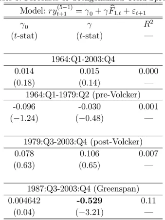
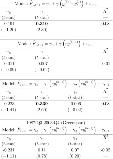
We now turn to the question of whether the term premium component of the yield spread we identify is related to real economic activity, as measured by the real factor Fb1t. Table 5 displays the results of univariate forecasting regressions of the orthogonalized innovations in the yield spread onto the lagged factor Fb1t, where we have estimated both the forecast error for the yield spread and Fb1t over the same sample used to estimate return risk premia above. Results for other factor are not reported since we …nd little relation between the risk premium component in yields and the other factors. The table shows thatFb1tis unrelated to the orthogonal component of future yields in the early subperiods, but is a strong predictor in the Greenspan period. This factor alone explains 11 percent of the variation inryt(5 1) one quarter ahead in the Greenspan period. Since Fb1t is positively correlated with measures of output and employment, these …ndings are qualitatively similar to those presented above for bond returns: they suggest that investors must be compensated for risks related to recessions or, conversely, that investors require lower risk premia in good times when the economy has been expanding.
The point estimate in the regression reported in Table 5 suggests that the a¤ect of Fb1t on risk premia in yields in the Greenspan period is economically large. A one-standard deviation increase in Fb1t leads to a decline of 0.48 in the orthogonalized yield spread. This implies a decline of greater than two standard deviations in the risk premium component of the term spread. Given the large fraction of variation in the short-term forecast error of yield spreads that is explained by this component in recent decades, these …ndings imply that much of