A Congestion Aware Ant Colony
Optimisation Based Routing and
Wavelength Assignment Algorithm for
Transparent Flexi-grid Optical Burst
Switched Networks
Joshua Femi Oladipo
Submitted in fulfilment of the requirements for the degree of Magister Scientiae
in the Faculty of Science Nelson Mandela University
December 2018
Declaration of Own Work
I, Joshua Femi Oladipo (210036575), declare that the entirety of the work contained in this dissertation is my own original work. That I am the sole author thereof (save to the extent explicitly otherwise stated). That reproduction and publication thereof by Nelson Mandela University will not infringe on any third party rights. And that I have not previously in its entirety or in part submitted it for obtaining any qualification.
Signature:
Date: 11 October 2018
Acknowledgements
This research would not have been possible without the support of certain key indi-viduals. Firstly, I would like to thank God for keeping and guiding me throughout the duration of this research.
I would like to express my sincere gratitude to my supervisors Dr Mathys du Plessis, and Prof. Timothy Gibbon, for their technical, moral and material support through-out the course of the research. I am truly grateful.
I would like to thank the department of computing sciences for providing the re-sources required for this research, and for encouragement from various staff members. I would like to thank Grant Woodford and Jean Rademakers, for assisting me with the technical hassles.
I would like to thank my family and friends for their support and understanding. Finally, I would like to thank George Mujuru, for his words of encouragement.
Abstract
Optical Burst Switching (OBS) over transparent flexi-grid optical networks, is con-sidered a potential solution to the increasing pressure on backbone networks due to the increase in internet use and widespread adoption of various high bandwidth ap-plications. Both technologies allow for more efficient usage of a networks resources. However, transmissions over flexi-grid networks are more susceptible to optical im-pairments than transmissions made over fixed-grid networks, and OBS suffers from high burst loss due to contention. These issues need to be solved in order to reap the full benefits of both technologies. An open issue for OBS whose solution would miti-gate both issues is the Routing and Wavelength Assignment (RWA) algorithm. Ant Colony Optimisation (ACO) is a method of interest for solving the RWA problem on OBS networks. This study aims to improve on current dynamic ACO-based solu-tions to the Routing and Wavelength Assignment problem on transparent flexi-grid Optical Burst Switched networks.
In order to pursue the objective stated in the previous paragraph, an OBS simulator, which is capable of simulating the operation of OBS on transparent flexi-grid optical networks, was built and validated. A literature review of ACO based solution to the RWA problem on OBS networks, lead to the selection of two algorithms (ACOR and FSAC) as potential candidates for further development. A performance evaluation of both lead to the selection of FSAC as the algorithm of choice for future develop-ment. Based on the results of the performance evaluation, weak points of the FSAC algorithm were identified. Incorporating congestion information into the FSAC was identified as an option which might remedy the weak points of the algorithm. The modifications made to FSAC, was found to improve the performance of FSAC, and hence was given the name CM-FSAC.
Contents
Declaration of Own Work i
Acknowledgements ii
Abstract iii
Table of Contents vii
List of Figures ix
List of Tables xi
List of Abbreviations xii
1 Introduction 1 1.1 Background . . . 1 1.2 Research Objective . . . 3 1.3 Context of Study . . . 4 1.4 Methodology . . . 5 1.5 Dissertation Structure . . . 7 2 Literature Review 9 2.1 Introduction . . . 9
2.2 Wavelength Division Multiplexing . . . 9
2.2.1 Flexi-grid . . . 10
2.2.2 Transparent WDM Networks . . . 12
2.2.3 Enabling technologies . . . 14
2.2.4 Optical Impairments . . . 15
2.3 Optical Burst Switching . . . 18
2.3.1 Optical Switching . . . 19
2.3.2 Burst Assembly . . . 20
CONTENTS v
2.3.3 Routing and Wavelength Assignment . . . 20
2.3.4 Bandwidth Reservation and Switching . . . 23
2.4 Simulation Principles . . . 25
2.4.1 Discrete Event Simulation . . . 26
2.4.2 Simulator Frameworks . . . 27
2.4.3 Reduced Link Load Model . . . 28
2.5 Ant Colony Optimisation . . . 30
2.6 Ant Colony Optimisation RWA Algorithms . . . 32
2.6.1 ACOR . . . 32 2.6.2 DABR . . . 34 2.6.3 ACRWA . . . 36 2.6.4 UCBRWA . . . 38 2.6.5 FSAC . . . 40 2.6.6 Discussion . . . 41 2.7 Conclusion . . . 43
3 Simulator Design & Validation 44 3.1 Introduction . . . 44
3.2 Motivation . . . 44
3.3 Problem formulation . . . 45
3.4 Selection of Simulator Framework . . . 46
3.5 Omnet++ Architecture . . . 46 3.6 Simulator Design . . . 47 3.7 Simulator Implementation . . . 49 3.7.1 Edge Node . . . 50 3.7.2 Core Node . . . 52 3.7.3 Fibre . . . 52 3.7.4 Super Node . . . 53 3.8 OBS Validation . . . 55 3.8.1 Validation Procedure . . . 55 3.8.2 Validation Results . . . 56
3.9 Effects of Flexi-grid and Impairments . . . 57
3.9.1 Experimental Procedure . . . 57
3.9.2 Results and Analysis . . . 58
3.10 Conclusion . . . 60
4 Initial Investigations 61 4.1 Introduction . . . 61
CONTENTS vi
4.2 Adaptation & Implementation of Algorithms . . . 62
4.3 Network Scenarios . . . 63
4.4 Parameter Study . . . 64
4.4.1 Experimental Procedure . . . 64
4.4.2 Results and Discussion . . . 66
4.5 Performance Comparisons . . . 73
4.5.1 Experimental Procedure . . . 73
4.5.2 Parameter Selection . . . 74
4.5.3 Overall Performance Comparison . . . 76
4.5.4 Timewise Performance Comparison . . . 78
4.6 Discussion . . . 82
4.7 Conclusion . . . 82
5 Proposed Improvements 84 5.1 Introduction . . . 84
5.2 Incorporating Route Congestion Information . . . 84
5.2.1 Congestion Estimation . . . 85
5.2.2 Incorporating Congestion . . . 86
5.2.3 Other Modifications . . . 87
5.3 Information Deprived FSAC . . . 87
5.4 Parameter Study . . . 88 5.4.1 CM1 . . . 89 5.4.2 CM2 . . . 91 5.4.3 CM3 . . . 92 5.4.4 ID-FSAC . . . 92 5.5 Performance Comparison . . . 95 5.5.1 Parameter Selection . . . 95
5.5.2 Overall Performance Comparison . . . 96
5.5.3 Timewise Performance Comparison . . . 101
5.6 Conclusion . . . 104
6 Conclusion 105 6.1 Introduction . . . 105
6.2 Research Contributions . . . 105
6.2.1 Development of a Flexi-grid OBS Simulator . . . 106
6.2.2 Improved ACO RWA Solution . . . 107
6.3 Limitations . . . 108
CONTENTS vii
6.5 Summary . . . 109
A Results 116 B Statistical Methods 123 B.1 Pearson Correlation Coefficient . . . 123
B.2 Mann-Whitney U Test . . . 123
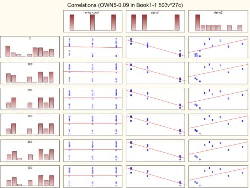
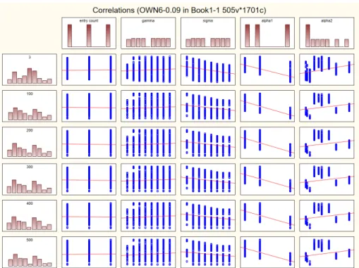
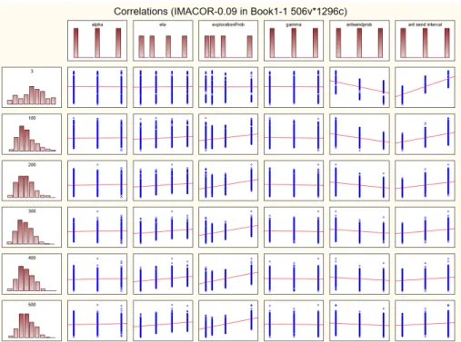
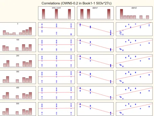
C CM-FSAC Pseudo-Code 124 D Scatter Plots of Data Obtained in Parameter Studies 127 D.1 NSFNET . . . 127 D.1.1 High . . . 127 D.1.2 Medium . . . 130 D.1.3 Low . . . 133 D.2 SIMPLE . . . 137 D.2.1 High . . . 137 D.2.2 Medium . . . 140 D.2.3 Low . . . 143 E IFIP PEMWN 2017 147
List of Figures
1.1 Steps in conducting a simulation study (Law, 2003) . . . 5
2.1 Illustration of fixed and flexi-grid (Miroslaw Klinkowski et al., 2013) . 12 2.2 The wavelength continuity constraint on a path that consist of two links. Used wavelengths are indicated in colour. (Shen & Yang, 2011) 14 2.3 Schematic view of various optical switching elements . . . 16
2.4 Illustration of the operation of Liquid Crystal on Silicon (LCoS) (L´opez & Velasco, 2016) . . . 17
2.5 Elastic wavelength assignment (Miroslaw Klinkowski et al., 2013) . . 24
2.6 Network timing diagrams, showing the operation of JIT and JET bandwidth reservation schemes. (Teng & Rouskas, 2003) . . . 25
2.7 Illustration of the shortest path finding ability of ant colonies (Blum, 2005) . . . 31
3.1 Simple and compound modules (“OMNET++ Simulation Manual”, 2018) . . . 46
3.2 Usage of simulator modules in building a network . . . 49
3.3 Edge Node components . . . 50
3.4 Core Node module layout . . . 51
3.5 Fibre module layout . . . 52
3.6 SuperNode module layout . . . 54
3.7 Network built using super nodes . . . 54
3.8 Topology used in validation, with routes used in validation . . . 55
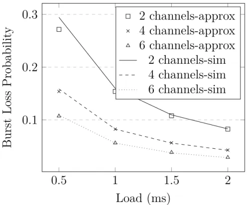
3.9 Graphs showing the average burst loss probability vs load, for the simulations and approximations . . . 56
3.10 NSFNET Topology (Gravett, du Plessis, & Gibbon, 2017). Link lengths in km. . . 58
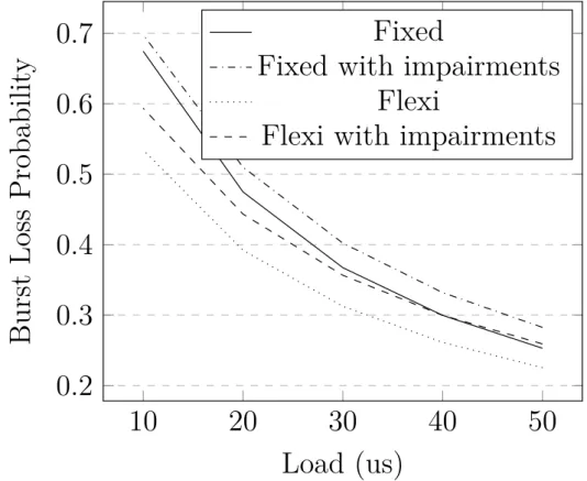
3.11 Graphs showing the average burst loss probability vs load, for various fixed and flexi-grid scenarios . . . 60
LIST OF FIGURES ix
4.1 SIMPLE Topology (Gravett, du Plessis, & Gibbon, 2017). Link
lengths in km. . . 63
4.2 Graphs showing the average Burst Loss Probability vs Spectrum
Width, for various algorithms on the SIMPLE topology at various loads . . . 77
4.3 Graphs showing the average Burst Loss Probability vs Spectrum
Width, for various algorithms on the NSFNET topology at various loads . . . 77
4.4 Time wise performance of algorithms on SIMPLE at various loads
with 100GHz spectrum width. . . 80
4.5 Time wise performance of algorithms on SIMPLE at various loads
with 200GHz spectrum width. . . 80
4.6 Time wise performance of algorithms on SIMPLE at various loads
with 300GHz spectrum width. . . 80
4.7 Time wise performance of algorithms on NSFNET at various loads
with 200GHz spectrum width. . . 81 4.8 Time wise performance of algorithms on NSFNET at various loads
with 300GHz spectrum width. . . 81 4.9 Time wise performance of algorithms on NSFNET at various loads
with 400GHz spectrum width. . . 81
5.1 Graphs showing the average burst loss probability vs Spectrum Width,
for various algorithms on the SIMPLE topology at various loads. . . 99
5.2 Graphs showing the average burst loss probability vs Spectrum Width, for various algorithms on the NSFNET topology at various loads. . . 99 5.3 Time wise performance of algorithms on SIMPLE at various loads
with 100GHz spectrum width. . . 102
5.4 Time wise performance of algorithms on SIMPLE at various loads
with 200GHz spectrum width. . . 102
5.5 Time wise performance of algorithms on SIMPLE at various loads with 300GHz spectrum width. . . 102 5.6 Time wise performance of algorithms on NSFNET at various loads
with 200GHz spectrum width. . . 103 5.7 Time wise performance of algorithms on NSFNET at various loads
with 300GHz spectrum width. . . 103
5.8 Time wise performance of algorithms on NSFNET at various loads
List of Tables
3.1 Burst Loss Probabilities obtained for various scenarios . . . 59
4.1 Parameter values used in parameter study of ACOR . . . 65
4.2 Parameter values used in parameter study of FSAC . . . 65
4.3 Mean inter-arrival time values used to achieve various loads in
pa-rameter studies . . . 66
4.4 Correlation coefficients for ACOR at various simulation times on the
SIMPLE topology. Significant values given in bold. . . 68 4.5 Correlation coefficients for ACOR at various simulation times on the
NSFNET topology. Significant values given in bold. . . 68 4.6 Correlation coefficients for FSAC at various simulation times on the
SIMPLE topology. Significant values given in bold. . . 72 4.7 Correlation coefficients for FSAC at various simulation times on the
NSFNET topology. Significant values given in bold. . . 72 4.8 Mean inter-arrival time values used to achieve various loads in
per-formance comparisons . . . 74 4.9 Parameter values used for ACOR in performance comparisons . . . . 75 4.10 Parameter values used for FSAC in performance comparisons . . . 75 4.11 Performance comparison of ACOR, FSAC and GSPR in cases with
statistically significant results. . . 78 5.1 Parameter values used in parameter study of CM1, CM2 and CM3. . 89 5.2 Parameter values used in parameter study of ID-FSAC . . . 89 5.3 Correlation coefficients for CM1 at various simulation times on the
SIMPLE topology. Significant values given in bold. . . 90 5.4 Correlation coefficients for CM1 at various simulation times on the
NSFNET topology. Significant values given in bold. . . 90
5.5 Correlation coefficients for CM2 at various simulation times on the
SIMPLE topology. Significant values given in bold. . . 90
LIST OF TABLES xi
5.6 Correlation coefficients for CM2 at various simulation times on the
NSFNET topology. Significant values given in bold. . . 93
5.7 Correlation coefficients for CM3 at various simulation times on the
SIMPLE topology. Significant values given in bold. . . 93
5.8 Correlation coefficients for CM3 at various simulation times on the
NSFNET topology. Significant values given in bold. . . 93
5.9 Correlation coefficients for ID-FSAC at various simulation times on
the SIMPLE topology. Significant values given in bold. . . 94 5.10 Correlation coefficients for ID-FSAC at various simulation times on
the NSFNET topology. Significant values given in bold. . . 94 5.11 Parameter values used for CM1, CM2 and CM3 in performance
com-parisons . . . 96 5.12 Parameter values used for ID-FSAC in performance comparisons . . . 97 5.13 Performance comparison of CM1, CM2, CM3, FSAC, GSPR, and
List of Abbreviations
Abbreviation Term
ACO Ant Colony Optimisation
BVT Bandwidth Variable Transponder
BLP Burst Loss Probability
CWDM Coarse Wavelength Division Multiplexing
DWDM Dense Wavelength Division Multiplexing
JET Just Enough Time
JIT Just-In-Time
LCoS Liquid Crystal on Silicon
OBS Optical Burst Switching
OCS Optical Circuit Switching
OEO Optical-Electrical-Optical
OPS Optical Packet Switching
OXC Optical Cross-Connect
RAM Random Access Memory
ROADM Reconfigurable Optical Add/Drop Multiplexer
RWA Routing and Wavelength Assignment
TTL Time-To-Live
WC Wavelength Continuity
WDM Wavelength Division Multiplexing
WSS Wavelength Selective Switch
Chapter 1
Introduction
1.1
Background
An optical network is a communication network which uses light signals to transmit data over glass fibres (called optical fibres). The potential bandwidth that could be accessed over optical fibre vastly outstrips that available over any other communica-tion medium currently in use; hence, they form a major part of telecommunicacommunica-tion backbone networks in the form of Wide Area Networks (WANs) and Metropolitan Area Networks (MANs) (Maier, 2008; Ramaswami, Sivarajan, & Sasaki, 2010). Op-tical fibre have also been increasingly deployed in Access Networks, where opOp-tical fibres are used up to the connections to homes and offices (Maier, 2008; Ramaswami et al., 2010; L´opez & Velasco, 2016).
Due to various technological limitations, the full potential of optical fibres are not currently being exploited. On the other hand, demand for network bandwidth is steadily and quickly increasing due to the increase in Internet access over fixed and mobile channels as well as the widespread adoption of various high bandwidth applications by end-users such as video streaming, cloud storage and cloud com-puting (L´opez & Velasco, 2016; Jinno et al., 2009). Network traffic patterns are also becoming more dynamic in time and direction; that is large changes in traffic magnitude as well as flow direction occur over the span of a day (L´opez & Velasco, 2016). These issues call for an increase in network capacity and flexibility.
Wavelength Division Multiplexing (WDM) is a method of increasing transmission capacity of an optical fibre by allowing the parallel transmission of multiple streams of data over the fibre (where each stream is sent on a different wavelength) (Maier, 2008; Ramaswami et al., 2010; Simmons, 2014). The two variations of WDM are
1.1. BACKGROUND 2 Coarse Wavelength Division Multiplexing (CWDM), where a maximum of 16 widely spaced wavelengths might be used; and Dense Wavelength Division Multiplexing (DWDM) where over 100 closely spaced wavelengths could be used (Stamatis V. Kar-talopoulos, 2004; Transmode, 2013). The wavelengths which should be supported by equipment that supports DWDM are standardised by the International Telecom-munication Union (ITU) in Recommendation G.694.1 (International Telecommuni-cation Union - ITU-T, 2012); The document defines a fixed grid scheme of various bandwidth spacing; as well as a flexible grid scheme (also known as flex spectrum) which allows the use of arbitrarily positioned and sized bandwidth channels, made up of smaller concatenated channels (whose size are multiples of 12.5GHz). The flexible grid scheme allows for more efficient usage of the bandwidth available over a fibre, however, it comes with a penalty in terms of increased inter-channel crosstalk due to the reduced guard bands between transmission channels on the fibre.
The use of Wavelength Division Multiplexing (WDM) and it’s corresponding optical transmission and switching technologies (such as Bandwidth Variable Transponders (BVT’s), Reconfigurable Optical Add Drop Multiplexers (ROADM’s) and Optical Cross Connects (OXC’s)) allow for reconfigurable optical networks; hence improving the flexibility of these networks. Researchers are presented with the opportunity to develop advanced control plane algorithms to derive maximum benefit from current optical networks, hence, reducing the need for capital expenditure spent to im-prove network capacity and performance. The availability of the above mentioned technologies (BVT’s, ROADM’s and OXC’s) lead to the proposal of new optical switching technologies which such as Optical Burst Switching and Optical Packet Switching which would improve the efficiency of optical networks.
Current optical networks use a switching paradigm known as Optical Circuit Switch-ing (OCS), where all the bandwidth on a channel (where a channel could be a fibre, a wavelength, or a time slot in a Time Division Multiplexed (TDM) system) is fully dedicated to transmission between a pair of nodes (Maier, 2008; Chen, Qiao, & Yu, 2004). The channels may be assigned statically or as required for a given amount of time. The disadvantage of this is that for bursty (irregular) data the bandwidth of a channel is reserved for a given node irrespective of if the node has data to transmit. A node might not need to send data or might only need to send data across a channel for a short period of time, leaving the remaining channel slot unused; while another application might currently need the bandwidth. This is inefficient. A better way would be to use Optical Packet Switching (OPS), where packets sent over a given wavelength channel are independently switched towards their destination (Maier & Reisslein, 2008; Rouskas & Xu, 2004). However, true OPS is not currently possible
1.2. RESEARCH OBJECTIVE 3 due to the absence of cost effective optical buffers, which would allow the buffering of packets to enable contention resolution at core nodes, as well as efficient meth-ods for processing each packet within the optical domain similar to what occurs on electronic packet switched networks (Maier & Reisslein, 2008; Rouskas & Xu, 2004).
Optical Burst Switching (OBS) could be considered a compromise to improve the efficiency of optical networks using currently available technology (Chen et al., 2004; Bjornstad et al., 2003; Verma, Chaskar, & Ravikanth, 2000). In an OBS network, packets are buffered and assembled into bursts at network edge nodes according to various parameters. When a burst is ready to be sent, the node sends a packet known as a Burst Control Packet (BCP), on a reserved channel called the control channel, in order to reserve the required bandwidth and configure the switches at intermediate nodes. The burst is then sent after a certain offset time, in order to give the BCP time to finish setting up the switches at the intermediate nodes. The reserved bandwidth for a transmission is released after the burst has traversed the network, in order to allow its use by another burst.
A major issue that needs to be solved in OBS networks is the Routing and Wave-length Assignment (RWA) problem. RWA deals with the routing and assignment of wavelengths in order to ensure that the current request is fulfilled, the Burst Loss Probability (BLP) of future requests is minimised and ensure that available network resources are used in an efficient manner (Gravett, du Plessis, & Gibbon, 2017). The RWA problem consist of two parts: computing a path from source to destination and then assigning a wavelength to the selected path. The RWA problem could be solved in the presence of the Wavelength Continuity (WC) constraint, where a single wavelength must be used to traverse the path from the source to the destination node or without it (Simmons, 2014; Rouskas, 1999). Enforcing the WC constraint offers the benefit of avoiding the costly optical to electrical conversion (and pos-sibly storage) which would be required at each node to deal with any wavelength contention that might occur.
1.2
Research Objective
Currently used technologies in optical networks are not sufficient to deal with the increasing demand for bandwidth and the new dynamic dimensions of this demand. Hence there is a need for new methods of data transmission in order to exploit im-proved technology and handle the demand. As presented in Section 1.1, OBS on
1.3. CONTEXT OF STUDY 4 flexi-grid networks is the most viable technology for the foreseeable future. How-ever, both technologies have issues that require solutions to manage them; that is, increased transmission impairments on flexi-grid and the Routing and wavelength assignment (RWA) problem for OBS.
A method of interest for solving the RWA problem is Ant Colony Optimisation (ACO). ACO is a set of algorithms that aim to emulate the emergent behaviour of ants foraging for food. It has been applied to various graph-theoretic problems, and is of interest due to its ability to dynamically route data while improving network performance, and to continuously adapt to changes on the network (such as changes in the number of available wavelengths, removal or addition of a node and increase or decrease in the amount of traffic). Hence the objective of this research is to improve on current dynamic ACO-based solutions to the Routing and Wavelength Assignment problem on flexi-grid optical burst switching networks. The improved solution should reduce the Burst Loss Probability (BLP) and effectively utilise and manage spectrum resources while also considering optical impairments, under the wavelength continuity constraint.
Pursuing the objective stated above will require the use of a discrete event simulator which simulates the operation of OBS over flexi-grid networks, while incorporating impairment modelling. However, in the course of preliminary research, no simulator which could fulfil the needs of the research could be found. Hence, a secondary objective of this research is to design and implement a flexible simulator which is capable of meeting the needs of OBS researchers.
1.3
Context of Study
This research will be conducted within the Centre for Broadband Communication (CBC) and falls under the “Next generation Dense Wavelength Division
Multiplex-ing (DWDM) systems research” focus area of the centre1. The CBC was created
with the support of the Department of Science and Technology (DST), the Na-tional Research Foundation (NRF), the Council for Scientific and Industrial Re-search (CSIR), the Square Kilometre Array (SKA) and Cisco, and is tasked with developing resources necessary to ensure that all South Africans have access to the Internet by 2020.
1More information on the Centre for Broadband Communication can be found at
1.4. METHODOLOGY 5
Figure 1.1: Steps in conducting a simulation study (Law, 2003)
1.4
Methodology
Theory related to WDM (focussing on flexi-grid, transparent networks, enabling technologies, and optical impairments), OBS, simulation and ACO are presented in Chapter 2. A literature review of existing ACO RWA algorithms for OBS networks is also performed in Chapter 2, in order to gain an understanding of the ways ACO has been applied to OBS networks.
The research will be performed using the seven step approach for successfully con-ducting a simulation study prescribed by Law (2003). The steps are presented in Figure 1.1 and explained below
1.4. METHODOLOGY 6 of the model, and the performance measures that need to be collected.
2. Collect information and construct conceptual model - collect informa-tion from real systems if possible; for use in constructing a conceptual model and validating the final system. The documentation of the conceptual model should include a detailed description of the operations of various subsystems as well as how they interact and the various assumptions made.
3. Check for conceptual model validity - discuss the conceptual model with stakeholders in a structured manner to determine any errors and omissions, and ensure that any assumptions made are correct.
4. Implement the model- implement the conceptual model either from scratch or using an appropriate simulation tool. Verify the program by debugging. 5. Check for implementation validity - compare the results obtained from
the tool against results from real world systems if available, or analytical re-sults. Results should be scrutinised to ensure they are reasonable, and analysis should be performed to determine the extent to which various factors affect the obtained results, to allow for careful implementation of the more influential factors.
6. Design, conduct and analyse experiments - determine configurations of interest and related factors such as the run length of experiments, and number of times to replicate them. Analyse the results to determine if more experiments are needed.
7. Document and present the simulation results - document conceptual models and implementation details as well as results from experiments. Pre-sentation of results should also clearly state their limitations.
Consequently, chapter 3 details the design, implementation and validation of an OBS simulator using a selected simulation frame work, hence, fulfilling steps one to five of the seven step approach.
Chapters 4 and 5 present the experimental design as well as results obtained from the experiments towards the main objective of this research as specified in Section 1.2. In Chapter 4, Two ACO RWA algorithms, which might undergo further development were selected from those previously discussed in Chapter 2. Parameter studies and performance evaluations were performed on both algorithms, in order to determine which performs best, and hence, which might be selected for further development. The algorithms were evaluated on two topologies with three load conditions. In Chapter 5, modifications which might improve the operation of the algorithm were
1.5. DISSERTATION STRUCTURE 7 proposed and implemented based on observations made about the best performing algorithm in the performance evaluations of Chapter 4. The proposed modifications were then evaluated against each other and the original algorithm, to determine, if an improvement had been achieved. Chapters 4 and 5 fulfil steps six and seven of the seven step approach.
1.5
Dissertation Structure
An outline of the contents of the various chapters of this dissertation is given below
Chapter 2 : Literature Review
Chapter 2 presents the applicable background theory of optical networks, OBS, simulator development and ACO. Various applications of ACO to RWA on OBS networks are reviewed.
Chapter 3 : Simulation Design & Validation
Chapter 3 details the process of designing, implementing and validating the simula-tor that was used in this research.
Chapter 4 : Initial Investigations
Chapter 4 details the initial evaluations of select ACO algorithms which were re-viewed in Chapter 2. They were evaluated in order to determine their performance against each other on flexi-grid OBS networks, and what improvements may be made to them. The algorithm which performs best in the evaluations is selected for future development.
Chapter 5 : Proposed Changes
In Chapter 5, various modifications which might improve the performance of the algorithm selected in Chapter 4 are made. The modified algorithm is evaluated against the original, in order to determine if there is a performance improvement.
Chapter 6 : Conclusions
In chapter 6, an overview of the research will be given. The contributions and limitations of this work will be stated. Finally, recommendations for future research are also proposed.
1.5. DISSERTATION STRUCTURE 8 Appendix A presents the comparison results collected for the various algorithms in tabular form.
Appendix B : Statistical methods
Appendix B presents a brief overview of the two major statistical techniques used in the course of the research.
Appendix C : CM-FSAC Pseudo-code
Appendix C presents the pseudo-code of the CM-FSAC algorithm generated by this research.
Appendix D : Scatter Plots of Data Obtained in Parameter Studies
Appendix D presents scatter plots of data obtained during parameter studies.
Appendix E : IFIP PEMWN 2017
Appendix E presents the conference paper that was accepted and presented at the 6th IFIP International Conference on Performance Evaluation and Modeling in Wired and Wireless Networks.
Chapter 2
Literature Review
2.1
Introduction
In this chapter, various aspects of the research are discussed. Wavelength Division Multiplexing is discussed in Section 2.2; focus is placed on its evolution, enabling technologies, and the various optical impairments which may occur. Next, the op-eration of Optical Burst Switching is described in Section 2.3; paying particular attention to the burst assembly, routing and wavelength assignment and switching aspects. Section 2.4 presents theory relating to simulations and an introduction to Discrete Event Simulation (Section 2.4.1). It was decided that a simulator frame-work would be used as opposed to building a simulator from scratch; in order to increase the speed of development, and obtain the credibility, usability and exten-sibility advantages which may be obtained from a framework. Hence, a survey of potential simulator frameworks which might be used in building the simulator re-quired for the research is given (Section 2.4.2); followed by an introduction to the method which will be used to validate the operation of the built simulator (Sec-tion 2.4.3). An introduc(Sec-tion to Ant Colony Optimisa(Sec-tion is given in Sec(Sec-tion 2.5. And lastly, a survey of Ant Colony Optimisation methods applied to Optical Burst Switched networks is performed in Section 2.6.
2.2
Wavelength Division Multiplexing
Wavelength Division Multiplexing (WDM) is a method of increasing the transmis-sion capacity of an optical fibre, by allowing the parallel transmistransmis-sion of multiple streams of data, with potentially different transmission speeds over different
2.2. WAVELENGTH DIVISION MULTIPLEXING 10 lengths across an optical fibre (Maier, 2008; Ramaswami et al., 2010; Simmons, 2014). This vastly increases the transmission capacity of optical networks.
In this section, a discussion of flexi-grid and transparent WDM networks is given. Followed by a brief overview of their enabling technologies and the optical impair-ments which may occur over optical networks.
2.2.1
Flexi-grid
WDM systems may adhere to either the Coarse Wavelength Division Multiplexing (CWDM) standard or Dense Wavelength Division Multiplexing (DWDM) standard of the ITU-T (Stamatios V. Kartalopoulos, 1999; Transmode, 2013). The standards prescribe what wavelengths WDM hardware should support, in order to foster inter-operability of hardware by different manufacturers. CWDM and DWDM are both fixed grid schemes; that is, the frequency spacing between the central frequency of adjacent wavelengths is kept constant (this spacing is called the channel spacing). CWDM is the earlier standard(International Telecommunication Union - ITU-T, 2003). CWDM requires that the wavelengths are widely spaced in order to reduce the impact of impairments on the transmissions; this was necessary due to the expense and immaturity of transponder and fibre technology at the time. Hence CWDM systems may only support a maximum of 18 wavelengths. As technology improved, the wavelengths could be moved closer together leading to DWDM (illustrated in Figure 2.1a) which allows for equipment that supports 12.5GHz, 25Ghz, 50Ghz and
100GHz spacings (Stamatios V. Kartalopoulos, 1999; International
Telecommu-nication Union - ITU-T, 2012). However, in practice 50GHz spacing (leading to networks with over a 100 wavelengths) has been favoured, as it allows for the trans-mission of signals with a transtrans-mission rate of 10-100Gb/s. However, the fixed grid spectrum is considered wasteful, due to the fact that transmissions often do not require the whole wavelength, leading to the presence of large guard bands (unused spectrum) (Wright, Lord, & Velasco, 2013; Xia, Gringeri, & Tomizawa, 2012). For example, a 10Gb/s transmission requires only 15GHz of spectrum, however, it has to be assigned the whole 50GHz (Xia et al., 2012).
Due to the increasing pressure on data networks, network operators are seeking ways of increasing their transmission capacity (Wright et al., 2013; Gerstel, Jinno, Lord, & Yoo, 2012; Xia et al., 2012). Hence, network operators are deploying higher transmission rates of 400Gb/s and higher, to handle high-bandwidth applications (Wright et al., 2013; Gerstel et al., 2012; Xia et al., 2012). However, the ITU-T fixed grid does not allow efficient transmission of high bit rate signals, as they do not fit
2.2. WAVELENGTH DIVISION MULTIPLEXING 11 into the prescribed 50GHz spectrum. For example, in order to transmit a 400Gb/s signal on a fixed grid, the signal could be split into four 100Gb/s signals, which would fit into 50GHz channels; however, this would use up 125GHz of spectrum more than if the signal had been transmitted using a single 400Gb/s signal (Wright et al., 2013). In order to be cost-effective, optical networks need to be multi-line rate networks, due to diverse nature of demands (diverse transmission rates, and hence, spectrum requirement) they have to serve and the trade-off between transmission rate and reach (Nag, Tornatore, & Mukherjee, 2010; Amaya et al., 2011; Wright et al., 2013). The trade-off between transmission rate and reach the distance a signal will travel without having to re-generated is dependent on its transmission rate; higher transmission rate signals are capable of travelling less distance than lower transmission rate signals (Nag et al., 2010; Amaya et al., 2011; Wright et al., 2013). It is important to limit the amount of signal re-generation performed due to the equipment cost and to minimise energy consumption of the network (Nag et al., 2010; Amaya et al., 2011; Xia et al., 2012).
Flexi-grid was specified in (International Telecommunication Union - ITU-T, 2012), in order to cater for the issues presented in the previous paragraphs (wastefulness in current networks due to large guard bands, deployment of increased transmission rates, and need to support multi-line rate networks). Flexi-grid finely specifies the wavelengths and allows the concatenation of adjacent wavelengths to make bigger channels (International Telecommunication Union - ITU-T, 2012). Figure 2.1 illus-trates the structure of the bandwidth over a link, on a fixed grid (Figure 2.1a) and flexi-grid (Figure 2.1b) network. Potential central frequencies are spaced out at 6.25 GHz; however, the channel spacing (channel segment in Figure 2.1b) is 12.5GHz. This difference in central frequency spacing and channel spacing is in order to allow the placing of channels whose width is an even multiple of 12.5GHz, next to one whose width is an odd multiple of 12.5GHz, without a gap. Any number of adjacent channels can be assigned to a transmission as long as they do not overlap with an-other already assigned channel. The number of channels required for a transmission is dependent on the transmission speed and modulation format.
Flexi-grid leads to more efficient usage of the available bandwidth, due to the fact that transmissions with large bandwidth requirements can grow as much, to use whatever they need (faster transmissions require more spectrum). While trans-missions with small spectrum requirements only use the minimum spectrum they require (Wright et al., 2013; Gerstel et al., 2012). Flexi-grid also makes the network more flexible and responsive to changes in the network hardware, evolving demands and improvements in technology (Wright et al., 2013; Gerstel et al., 2012). The
2.2. WAVELENGTH DIVISION MULTIPLEXING 12
(a) Fixed DWDM Grid
(b) Flexi-grid
Figure 2.1: Illustration of fixed and flexi-grid (Miroslaw Klinkowski et al., 2013) channel spacings of flexi-grid also allow it to be compatible with DWDM systems; hence easing the adoption process. However, due to the lack of large guard bands as are present in fixed grid systems, the impact of impairments (particularly inter-channel cross-talk) which might prevent signals from reaching their destination is more prominent than in flexi-grid systems (Wright et al., 2013; Gerstel et al., 2012). Flexi-grid is an example of flex-spectrum transmission. Where flex-spectrum is a generic term used in the literature for optical transmission systems where the spectrum may be assigned arbitrarily with or without the guidance of an ITU-T grid. Another type of flex-spectrum is grid-less (Shen & Yang, 2011), where arbitrarily sized and positioned spectrum can be assigned to transmissions on the network. Grid-less has all the advantages and disadvantages of flexi-grid, except that it isn’t supported by the ITU-T and is not compatible with the DWDM systems.
2.2.2
Transparent WDM Networks
WDM networks can be classified as opaque, transparent or translucent (Maier, 2008; Saleh & Simmons, 2012; Simmons, 2014). In opaque networks, Optical-Electrical-Optical (OEO) conversion occurs at each node; all incoming optical wavelength channels are converted to electrical signals before being retransmitted across an-other link if they have not arrived at their destination. This allows for wavelength
2.2. WAVELENGTH DIVISION MULTIPLEXING 13 conversion at intermediate nodes (that is switching a transmission from its current wavelength to a free one, if it current wavelength is being occupied by another transmission) and retransmission at intermediate nodes, hence improving the reach of transmissions. On the other hand, in transparent networks (also called All-Optical Networks), intermediate nodes on the way to the destination can be optically by-passed by optical wavelengths which have not arrived at their destination, while transmissions terminating at that node are converted to electrical signals. Thus a transmission between two nodes can traverse the network without undergoing OEO transmission. Translucent networks are simply WDM networks which have a mix of transparent and opaque nodes.
Transparent networks are more scalable and reliable than opaque networks due to large reduction in required electronics (particularly transponders) yielding reduced cost, space, heat dissipation and power requirements (Maier, 2008; Saleh & Sim-mons, 2012; SimSim-mons, 2014; Jinno et al., 2009). They are also much easier to extend, as extending a node only requires the addition of more optical transponders (Maier, 2008; Saleh & Simmons, 2012; Simmons, 2014; Jinno et al., 2009). Finally, and most importantly, they are agnostic to the wavelength, modulation scheme, line rate and protocol being used; that is in an opaque network every node needs to support all transmission line rates and modulation format (Maier, 2008; Saleh & Simmons, 2012; Simmons, 2014; Jinno et al., 2009). However, in a transparent optical network, only the source and destination nodes need to support the formats being used for transmission. All the above advantages make transparent networks an attractive proposal to network operators, as they are more flexible and cheaper to operate than opaque networks (Maier, 2008; Saleh & Simmons, 2012; Simmons, 2014; Jinno et al., 2009).
Disadvantages of transparent networks are: transmissions are not regenerated due to absence of OEO conversion at each node, hence increasing the effects of impairments on transmissions (potentially reducing the reach of transmissions) and reducing the performance monitoring ability of the network (Maier, 2008; Saleh & Simmons,
2012; Simmons, 2014). An incoming transmission into a network would tie up
a wavelength across multiple links, preventing the wavelength from being used by subsequent transmissions which arrive within the duration of the first transmission and have intersecting paths on the network. This is called the Wavelength Continuity (WC) constraint (Maier, 2008; Saleh & Simmons, 2012; Simmons, 2014). In Figure 2.2, the WC constraint on a path with two links is illustrated. It can be observed that the actual amount of spectrum which may be assigned to a transmission which would travel across Link 1 and Link 2 (indicated as “Lightpath”) is less than the
2.2. WAVELENGTH DIVISION MULTIPLEXING 14
Figure 2.2: The wavelength continuity constraint on a path that consist of two links. Used wavelengths are indicated in colour. (Shen & Yang, 2011)
free amount of spectrum on Link 1 and Link 2; the spectrum that may be assigned to a new transmission, excludes those already assigned to other transmissions on either of the links.
The wavelength continuity constraint has the implication that transmissions might be lost even though there are enough wavelengths available on the required links; due to the necessary wavelength being occupied along the route of the transmission. In flexi-grid networks, the WC constraint also leads to fragmentation, where due to the mixture of transmissions with various transmission speeds on the network (faster transmissions require more spectrum), free spectrum along a route can become iso-lated, hence preventing the assignment of such spectrum to new transmissions due to the isolated wavelengths not being large enough to service new requests (Wright et al., 2013; Simmons, 2014).
The wavelength continuity constraint can only be eliminated by wavelength conver-sion of blocked transmisconver-sions at intermediate nodes (Maier, 2008; Saleh & Simmons, 2012; Simmons, 2014). Sadly, all-optical wavelength converters are still immature and expensive technology, hence the only practical way of achieving this is by in-troducing OEO conversion at intermediate nodes to service blocked transmissions (Maier, 2008; Saleh & Simmons, 2012; Simmons, 2014). However, this has the disadvantage of reducing the benefits obtained from transparent networks, as stated above.
2.2.3
Enabling technologies
The dynamically configurable technologies enabling All-optical flexi-grid networks are Bandwidth Variable Transponders (BVT’s), Reconfigurable Optical Add Drop Multiplexers (ROADM’s) and Optical Cross-connects (OXC’s) (Maier, 2008;
Ra-2.2. WAVELENGTH DIVISION MULTIPLEXING 15
maswami et al., 2010; Simmons, 2014). BVT’s allow for the transmission and
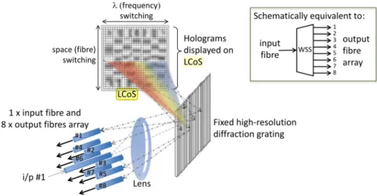
receiving of data on arbitrarily sized and positioned wavelengths within the sup-ported range, using various modulation formats (Maier, 2008; Ramaswami et al., 2010; Simmons, 2014). This allows the delivery of data at multiple data rates. ROADM’s and OXC’s allow for the switching of arbitrary single wavelengths at a node from link to link, and allow the addition and removal of a transmission into and out of the network, respectively (Maier, 2008; Ramaswami et al., 2010; Simmons, 2014). Figure 2.3a and 2.3b show a schematic view of an opaque and transparent OXC, respectively. The difference between both is that in an opaque OXC, the in-coming transmission is converted to electrical signals before being retransmitted on the appropriate link, transmissions that should be taken off the network are removed in the electronic domain; while in the transparent OXC all switching is performed in the optical domain with transmissions that should be taken off the network, di-rected optically towards an output transponder. The difference between ROADM’s and OXC’s is that ROADM’s are only degree two (where the degree of a node is the number of links that leave a node); hence they are used in linear scenarios such as point to point links and ring networks, while OXC’s are multi-degree allowing for use in mesh networks (Maier, 2008; Ramaswami et al., 2010; Simmons, 2014). A schematic of the operation of transparent ROADM’s is shown in Figure 2.3c. The flexibility offered by ROADM’s and OXC’s also enables new switching technologies such as Optical Burst Switching (OBS) and Optical Packet Switching (OPS). The key technology that enable transparent ROADM’s and OXC’s is the Wavelength Selective Switches(WSS); in the case of flexi-grid, specifically the Liquid Crystal on Silicon (LCoS) based WSS (L´opez & Velasco, 2016; Tomkos, Azodolmolky, Sol´e-Pareta, Careglio, & Palkopoulou, 2014; Fernandez-Palacios, L´opez, Cruz, & De Dios, 2014). A representation of the operation of LCoS Switches is given in Figure 2.4. Light to be switched from an input port is directed onto a diffraction grating which splits the light into its constituent wavelengths; the resulting wavelengths are then directed and spatially spread out onto the LCoS, where they are reflected into the appropriate output fibre (L´opez & Velasco, 2016). The angle at which a wavelength is reflected from the LCoS determines what fibre it will be sent into. This angle is determined by the pattern displayed on the LCoS.
2.2.4
Optical Impairments
When designing optical WDM networks, certain physical effects which may prevent transmissions from being received at their destinations occur as a result of the
2.2. WAVELENGTH DIVISION MULTIPLEXING 16
(a) Opaque Optical Cross-connect (Luke, Larsen, Ehrhardt, & Jansen, 2005)
(b) Transparent Optical Cross-connect (Luke, Larsen, Ehrhardt, & Jansen, 2005)
(c) Reconfigurable Optical Add Drop Multiplexer (Ramaswami, Sivarajan, & Sasaki, 2010)
2.2. WAVELENGTH DIVISION MULTIPLEXING 17
Figure 2.4: Illustration of the operation of Liquid Crystal on Silicon (LCoS) (L´opez & Velasco, 2016)
interaction between the light signals and the optical fibre. They may be classified
as either Linear or Non-linear (Shaw, 2004; Maier, 2008; Azodolmolky et al.,
2009). Linear impairments are independent of the power of a transmission and are proportional to the length of the fibre. Non-linear impairments are dependent on the number and power of the various transmissions on a fibre, as well as details such as the modulation format and the speed of each transmission. Some optical
impairments which may occur on optical fibres are (Shaw, 2004; Maier, 2008;
Azodolmolky et al., 2009)
• Attenuation where the received signal strength is weakened over a length of fibre compared to its strength when sent, due to slight manufacturing and splicing defects.
• Dispersion where different components of the transmitted signal travel at different speeds within the fibre and arrive out of phase with each other due to the various optical characteristics of the fibre. This causes the transmitted pulse to widen leading to inter-symbol interference which may prevent the transmitted data from being readable at the receiver. This limits the maximum transmission speed and is dependent on the length of the fibre.
• Cross-talk where signals from different channels interfere with each other.
• Non-linearities are effects that occur at high power levels due to scattering effects caused by molecular vibrations and refractive properties of the fibre.
2.3. OPTICAL BURST SWITCHING 18 In this research, the optical impairments which are going to be considered are At-tenuation and Cross-talk. Noise within electrical components will not be considered in the simulations as it is not of interest to solving the RWA problem. Dispersion will also not be considered, due to the fact that there are well established meth-ods to deal with dispersion (such as dispersion compensating fibre) in currently deployed networks (Stamatis V. Kartalopoulos, 2004). In order to model the power penalty (in decibels (dB)) experienced by a transmission across a fibre link due to attenuation and cross-talk; the following equation will be used (Boiyo et al., 2015)
P enalty(dB) =AL+cL X i∈Tf{s} bs10 Pi 10 bi10 Ps 10(fi−fs) (2.1)
where the constant c = 4.78 (Assuming On-Off keying modulation), A is the
at-tenuation constant in dB/km, L is the fibre length in km, Tf is the set of signals
traversing the fibre between the start and end time of the signal,bs is the bit rate of
the signal,bi is the bit rate of the signal causing the interference, Pi is the power of
the signal causing the interference in dBm,Ps is the power of the signal in
decibel-milliwatts (dBm), (fi −fs) is the difference between the central frequencies of the
interfering signal and the signal in GHz.
The penalty on the power of a transmission over a length of fibre, due to the effects of other simultaneous transmissions on the length of fibre, as well as due to the effects of attenuation can be obtained by using equation (2.1). The obtained penalty can then be subtracted from the power of the transmission at its source, to obtain the power that will be sensed by a receiver at its destination. If the power of the transmission at the destination is less than the receiver sensitivity at the destination, then the transmission is considered lost.
2.3
Optical Burst Switching
In this section, a review of the various optical switching paradigms is given, followed by an in depth description of the operation of burst assembly, routing and wavelength assignment and bandwidth reservation and burst switching.
2.3. OPTICAL BURST SWITCHING 19
2.3.1
Optical Switching
Current optical networks use a switching paradigm known as Optical Circuit Switch-ing (OCS), where all the bandwidth on a channel (where a channel could be a fibre, a wavelength, or a time slot in a Time Division Multiplexed (TDM) system) is fully dedicated to transmission between a pair of nodes (Maier, 2008; Chen et al., 2004). The channels may be assigned statically or as required for a given amount of time. The disadvantage of this is that, for bursty (irregular) data, the bandwidth of a channel is reserved for a given node, irrespective of if the node has data to transmit. A node might not need to send data, or might only need to send data across a channel for a short period of time, leaving the remaining channel slot unused, while another application might currently need the bandwidth. This is inefficient. A bet-ter way would be to use Optical Packet Switching (OPS), where packets sent over a given wavelength channel are independently switched towards their destination (this is known as statistical multiplexing) (Maier & Reisslein, 2008; Rouskas & Xu, 2004). However, true optical packet switching is not currently possible due to the absence of cost effective optical buffers which would allow the buffering of packets to enable contention resolution at core nodes, as well as efficient methods for pro-cessing each packet within the optical domain (Maier & Reisslein, 2008; Rouskas & Xu, 2004).
Optical Burst Switching (OBS) could be considered as a compromise to improve the efficiency of optical networks using currently available technology (Maier & Reisslein, 2008; Bjornstad et al., 2003; Battestilli, Perros, & Carolina, 2003; Verma et al., 2000). In an OBS network, packets are buffered and assembled into bursts, at network edge nodes, according to various parameters. When a burst is ready to be sent, the node sends a packet, known as a Burst Control Packet (BCP) on a reserved channel called the control channel, in order to reserve the required bandwidth and setup the switching at intermediate core nodes. The burst is then sent after a certain offset time, in order to give the BCP time to finish setting up the switching at the intermediate nodes. The reserved bandwidth for a transmission is released after the burst has traversed the network, in order to allow its use by another burst. OBS leads to more efficient usage of network resources, since bandwidth on the network is not tied up at any node for a long period, like in OCS. OBS has been shown to offer higher data throughput and lower blocking rates compared to OCS in simulation studies performed by Fei, Yoo, Yokoyama, and Horiuchi (2005) and Liu, Qiao, Yu, and Gong (2006)
2.3. OPTICAL BURST SWITCHING 20
2.3.2
Burst Assembly
Burst assembly deals with the aggregation of packets into data bursts at the edge nodes (Maier & Reisslein, 2008; Chen et al., 2004; Battestilli et al., 2003). Burst assembly algorithms could be time based; where only packets that arrive within a predefined period are sent. Burst size based; where the burst is sent once it reaches a predefined minimum size; a mix of both time based and burst size based, where a burst is sent depending on which parameter is satisfied first; or dynamic where either the burst assembly time or burst size is determined dynamically based on network conditions. Burst assembly is important because long bursts hold network resources for long time periods and may therefore cause higher burst losses due to contention, while short bursts increase network overhead because of the increased number of control packets that need to be processed.
2.3.3
Routing and Wavelength Assignment
Burst loss in an OBS network can occur due to two factors, wavelength contention between two or more burst reservations on a route (leading to the loss of at least one burst), and linear and non-linear optical impairments that could render the data sent in a burst unreadable at the destination node (Miroslaw Klinkowski et al., 2010; Azodolmolky et al., 2009). Routing and wavelength assignment deals with selecting a route-wavelength combination that will ensure that the current request is fulfilled, the blocking probability of future requests is minimised, that available network resources are used in an efficient manner (Gravett et al., 2017). To that end, routes and wavelengths for a request should be assigned so that they do not contend with existing transmissions on the network; they go through the smallest number of hops and use the least amount of bandwidth possible, to reduce the probability of blocking subsequent transmissions; and they use the shortest paths, in order to minimise the effects of impairments and reduce the latency of the network.
Routing and wavelength assignment on an OBS network could either be static or dynamic (Miroslaw Klinkowski et al., 2010). If it is static then predefined routes and wavelengths for each source-destination pair are pre-computed and bursts between two nodes are sent along their predefined routes. If routing is dynamic, a route will have to be computed or selected for each bursts; this allows the network to automatically respond to varying loads (by allowing the reassignment of unused resources to transmissions which require it) and detrimental events (for instance, the failure of a node might lead the network to use a different route for transmission
2.3. OPTICAL BURST SWITCHING 21 which go through the failed node). Routing might be performed at in a distributed manner, at each intermediate node (hereby referred to as node-by-node) or at the source edge node (hereby referred to as source routing) (Miroslaw Klinkowski et al., 2010). In a centralised routing protocol the BCP is sent to a central control node which keeps track of the resources available at each node as well as the network topology. The central control node determines the route that the burst will be sent over and reserves the bandwidth resources at each intermediate node. A centralised protocol is potentially more effective at minimising the Burst Loss Probability (BLP) as the central node has near perfect knowledge of the network state. However, the disadvantages of this is the high control overhead due to the high number of transmissions between the central node and every other node on the network (this also means that the central node is going to have to be equipped with high processing capabilities as it is going to need to process request for every node in the network); there will also be an increase in the latency of the network, due to the requirement that nodes wait for the response of the central node.
Routing and wavelength assignment algorithms may be classified based on the strat-egy they use in order to improve the performance of a network. RWA algorithms may be considered to be (Miroslaw Klinkowski et al., 2010)
• Withsingle path routing algorithms, the algorithm uses a single path for all transmissions between a source and a destination. This path may be statically set or may be dynamically selected as network conditions change.
The primary example of static single path routing is Shortest Path Routing (SPR). Transmissions between two nodes are sent along the shortest path which was pre-computed offline by an algorithm like Djikstra’s.
• Withmulti-pathrouting, a set of paths are used to send information between a source and destination in order to try and balance the load across the links of the network. In static routing, preset routes are determined, and assigned to transfer a certain portion of the traffic. In dynamic scenarios the path to be used is selected for each burst.
• Deflection routing can be used in conjunction with single and multi-path algorithms. However, when a wavelength contention occurs, the node at which contention occurs seeks to reschedule the burst on another link which is cur-rently free. The links to which the burst may be rescheduled may be deter-mined statically or dynamically. If static (commonly know as Fixed Alternate (FA) routing), the possible alternative links are pre-determined and fixed. To select an alternative link, the first alternative link found with the required free
2.3. OPTICAL BURST SWITCHING 22 wavelength is selected or a link is randomly selected from the set of alternate links on which the required wavelength is available. Alternative links with the required wavelengths available on them could also be chosen based on the shortest path to the destination which may be achieved through them.
If dynamic then the node uses knowledge of the wider network to compute a path towards a burst destination and push the burst towards its destination. An example of dynamic deflection routing is Fixed Alternate (FA). In FA, if an available wavelength can’t be found on the shortest path, the shortest available path with a free wavelength is used.
Assigning wavelengths in fixed grid networks is relatively straight-forward, as a free wavelength slot is simply assigned to a transmission. However, in a flexi-grid network, the amount of spectrum assigned needs to be variable in order to cater for multiple transmission rates. When assigning wavelengths to transmissions, the assigned wavelengths must be contiguous and should not overlap with those assigned to other transmissions. Figure 2.5 shows the various methods of catering for the varying spectrum requirements of transmissions presented by (Miroslaw Klinkowski & Walkowiak, 2011). Each method is described below
• Usingfixed wavelength assignment, the spectrum is split into chunks large
enough for the largest demands, and a transmission is simply assigned to one of these chunks. This is equivalent to fixed-grid transmission and negates the benefits of flexi-grid.
• Usingsemi-elastic wavelength assignment, the central frequencies are
pre-selected; however, the assigned spectrum is allowed to grow symmetrically around this central frequency. This is better as it allows for varying size transmission wavelengths; however, it still doesn’t fully exploit the benefits of flexi-grid.
• Theelastic wavelength assignmentapproach allows for free selection of the central frequency and channel size. In practice this is performed by selecting a potential centre and expanding the channel as required upwards or down-wards if possible, then finally, recalculating the centre of the newly selected wavelength. If there is no room for expansion, the centre frequency may be chosen at another location on the spectrum.
Four basic heuristics, which may be used to select a wavelength when performing fixed wavelength assignment, or the wavelength centre when performing semi-elastic and elastic wavelength assignment are (Zang, Jue, Mukherjee, et al., 2000)
2.3. OPTICAL BURST SWITCHING 23
• Random - a free wavelength is selected randomly with uniform probability.
• First-Fit - wavelengths are numbered sequentially, from the lower limit of the available spectrum to the upper limit. When searching for a free wavelength, the wavelengths are considered in ascending order, with the first free one being selected. The idea behind first-fit is to pack all current transmissions towards the beginning of the spectrum range, hence increasing the probability that more wavelengths will be available at the higher end of the spectrum to be used for longer transmissions.
• Least-Used- this heuristic determines which of the currently available wave-lengths is the least used wavelength on the network, and assigns this to new transmissions in an attempt to balance transmissions among all wavelengths. It requires global knowledge of how many times each wavelength has been used.
• Most-Used- this heuristic determines which of the currently available wave-lengths is the most used wavelength on the network, and assigns this to new transmissions. Its goal similar to first fit is to pack all transmissions within a small region of the spectrum, in order to allow more wavelength for longer transmissions. It requires global knowledge of how many times each wave-length has been used.
Two simple greedy algorithms for RWA is the combination of SPR with random wavelength selection or First-Fit wavelength selection.
2.3.4
Bandwidth Reservation and Switching
The protocol to reserve the network bandwidth could be either distributed or cen-tralised. In a distributed protocol, the edge node sends the BCP to the first node on the way towards the destination address, the first node then passes on the BCP to the next node and so on until the BCP reaches the destination address.
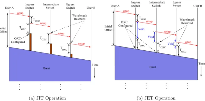
The bandwidth reservation and switching in intermediate nodes can be performed in two ways; Just-In-Time (JIT) and Just Enough Time (JET) (Chen et al., 2004; Teng & Rouskas, 2003; Kirci & Zaim, 2006). In JIT (Figure 2.6a), the intermediate nodes perform the bandwidth reservation and switching immediately after they receive the BCP. The bandwidth is reserved for the whole period of the transmission of the burst, and any request that come in for that wavelength during that period is discarded. In JET (Figure 2.6b), the intermediate node use the offset time carried by the
2.3. OPTICAL BURST SWITCHING 24
Figure 2.5: Elastic wavelength assignment (Miroslaw Klinkowski et al., 2013) BCP to perform the switching operation at the last possible moment. A burst is successfully scheduled using JET if the reservation request is for a time period after the last use of the wavelength or if the reservation request will fit into a time gap (void) between the end of a burst transmission and the start of the next one. There are various scheduling algorithms for JET such as Horizon and LAUC-VF; each with time complexity and bandwidth utilisation benefits (Nleya & Mutsvangwa, 2014). Teng and Rouskas (2003) and Kirci and Zaim (2006), recommend the use of JIT over JET due to its simplicity of implementation and similarity in performance over current hardware which have switching speeds in the millisecond range. Teng and Rouskas (2003) performs an analytical study of JIT and JET to determine in what range their performance are equivalent; they then perform computer simulations to determine the BLP over a variety of simulations and find the performance of JIT and JET to be comparable, particularly in scenarios with a small number of wavelengths. Kirci and Zaim (2006) performs simulations to compare JIT and JET over various network scenarios, and finds their performance to be comparable and the difference in performance to be nearly constant across all scenarios tested. The offset time between the BCP and burst transmissions is (Teng & Rouskas, 2003)
2.4. SIMULATION PRINCIPLES 25
(a) JIT Operation (b) JET Operation
Figure 2.6: Network timing diagrams, showing the operation of JIT and JET band-width reservation schemes. (Teng & Rouskas, 2003)
Where n is the number of core nodes on the selected route, Tsetup is the amount of
time required for BCP processing at each core node, andTOXC is the switching time
required by the last core node.
Bandwidth reservations may be released at each node in two ways; either the edge node sends a trailing release control message after the burst transmission, or the core nodes use their knowledge of the offset time and the length of the burst to estimate the time after which they may safely release the reserved bandwidth (Battestilli et al., 2003; Nleya & Mutsvangwa, 2014).
2.4
Simulation Principles
A simulator is an imitation of a complex entity, system, phenomena, or process, in order to study its behaviour (Guizani, Rayes, Khan, & Al-fuqaha, 2010; Banks, Nelson, Carson, & Nicol, 2010). A simulator typically employs one or more models in order to functionally represent a real world system to some degree of accuracy; where a model is a representation of a system for the purpose of studying that system (Guizani et al., 2010; Banks et al., 2010; Sokolowski & Banks, 2009). Simulators are often used to study systems which are too complex to study analytically; and too expensive to study in the real-world. They allow observers to obtain insight into how the various aspects of a system affect each other and their relative importance to
2.4. SIMULATION PRINCIPLES 26 the functioning of the system (Guizani et al., 2010; Banks et al., 2010; Sokolowski & Banks, 2009). Simulators also allow designers test the performance of new system designs (Guizani et al., 2010; Banks et al., 2010; Sokolowski & Banks, 2009), hence aiding the design process.
In this section, a brief introduction to Discrete Event Simulation (DES) is presented, followed by a brief introduction to the various simulator frameworks which might be used to build the OBS simulator. Finally, the Reduced Link Load model which will be used to validate the OBS simulator is described.
2.4.1
Discrete Event Simulation
Simulation models can either be discrete or continuous (Guizani et al., 2010; Banks et al., 2010; Sokolowski & Banks, 2009). A model is continuous if the state variable change continuously over time while a system is considered to be discrete only if the state variables change at a discrete, finite set of points in time. Computing and computer network systems are often modelled discretely, while biological and ecological systems are often modelled continuously. No real life system can be fully modelled exactly discretely or continuously; however, what determines what kind of model is used, is what behaviour the researcher is most interested in.
DES involves simulating a finite sequence of events, where each event is atomic (that is it leaves the system in a consistent state) and has a specific start and end time. The major components of a DES are an event queue, which keeps track of all events waiting to happen in the future; State variables which together completely describe the state of the system, and a simulation clock which keeps track of the global simulated time. Events are instantaneous occurrences which might change the state of the system. Events may create other events. The simulation clock can be advanced in an event driven manner or in a fixed increment manner. If done in a fixed increment manner; time is divided into small, fixed increments and all events occurring within each increment are processed before moving the simulation time forward. If done in an event driven manner; time is incremented to the start time of the next event in the event queue, after this event is processed, the clock is set to the time of the next event. The event driven manner is more efficient, particularly in scenarios where the time between inactive periods is large.
2.4. SIMULATION PRINCIPLES 27
2.4.2
Simulator Frameworks
In this section, three free, open-source simulator frameworks which may be used to develop an OBS simulator are described. These three were chosen, due to the fact that they are actively being developed, they already have pre-built libraries simulating real world protocols, and they are conducive to large scale simulation studies (that is, simulation studies with lots of runs).
2.4.2.1 Omnet++
The Omnet++ framework is an open-source, Discrete Event Simulator framework that can be used to build simulations for different scenarios (not just communication networks) (“Omnet++ Discrete Event Simulator - Home”, 2016; Andr´as Varga & Hornig, 2008; Andras Varga, 2010). Omnet++ uses a component based architec-ture, which allows for easier development of a simulation as key aspects of a model can be identified and implemented in separate modules. Modules may be nested in other modules to aggregate their behaviours and communication between modules is done via messages passed between modules. Development of modules is done using C++ and a module description language call NED, which is used to define the structure, parameters and connections of modules. NED is also used to define topologies, data collection and input parameters to simulations.
Omnet++ is well documented which makes the API easy to learn. It also has a sizeable active community as well as multiple open-source, community written simulation models (most notably the INET framework (“INET Framework”, 2018) which models various network protocols). It provides an Eclipse based IDE which allow for developing of modules in C++ and NED, as well as data analysis of result files obtained from simulations. Data analysis may also be done in R using the plug-in provided by the developers. The framework provides a graphical user plug-interface for simulations, which may be used to trace the operation of simulations and find errors while the simulation is under-way, hence, easing debugging.
2.4.2.2 IKR
IKR is an open-source, Discrete Event Simulator framework, which uses a com-ponent based architecture (“Institute of Communication Networks and Computer Engineering (IKR) - IKR Simulation and Emulation Library”, 2017; Sommer & Scharf, 2010). The framework provides a C++ and Java version. The framework