2019
Acceptée sur proposition du jury
pour l’obtention du grade de Docteur ès Sciences par
ILIJA BOGUNOVIC
Présentée le 25 janvier 2019Thèse N° 9147
Robust Adaptive Decision Making: Bayesian Optimization and
Beyond
Prof. E. Telatar, président du jury
Prof. V. Cevher, Prof. J. D. Haupt, directeurs de thèse Prof. S. Jegelka, rapporteuse
Prof. A. Krause, rapporteur Prof. M. Kapralov, rapporteur
à la Faculté des sciences et techniques de l’ingénieur Laboratoire de systèmes d’information et d’inférence Programme doctoral en informatique et communications
Acknowledgements
This thesis would not have been possible without the help and support of many people. First and foremost, I would like to express my gratitude to my advisor Volkan Cevher whose constant guidance and support have pushed me forward throughout my PhD. I really enjoyed my time in Volkan’s lab and I learned so much from him. Thank you Volkan for introducing me to the interesting topics in machine learning and optimization, for your research enthusiasm, for many research discussions and ideas, for your patience, optimism and valuable advice.
I would also like to thank my co-advisor Jarvis Haupt for his kindness, valuable discussions and for hosting me during my short stay at the University of Minnesota.
I was honored to have Stefanie Jegelka, Michael Kapralov, Andreas Krause and Emre Telatar as members of my thesis committee. I am grateful for their time and valuable discussions. Moreover, I am thankful to Stefanie for hosting me at MIT during the fall semester in 2017, and for providing an excellent and welcoming working environment. I sincerely enjoyed and learned a lot from our collaboration. I would also like to thank Volkan for arranging and making this research visit possible. I am also grateful to Andreas Krause for our collaboration, many valuable discussions and for introducing me to the area of machine learning.
I have been fortunate to collaborate with a number of brilliant colleagues at EPFL and LIONS lab. A special thanks go to Jonathan Scarlett for all our amazing collaborations. I truly enjoyed working together and I learned so much from him. His work directly contributed to the content of this thesis, and without him, the work in this form would not have been possible. Thank you Jonathan for your friendship, for the countless inspiring research discussions, for taking the time to review this manuscript, and for your valuable and thorough feedback. I am also grateful to my co-authors Junyao Zhao and Slobodan Mitrovic whose efforts have directly contributed to the content of certain chapters in this thesis. Moreover, I am sincerely thankful to all my lab members for our collaborations and research discussions: Yen-Huan Li, Paul Rolland (who also worked out the French abstract of this thesis), Luca Baldassarre, Anastasios Kyrillidis, Baran Gozcu, Marwa El-Halabi, Alp Yurtsever, Kamal Parameswaran, Chen Liu, Fabian Lattore as well as the other previous and current members of LIONS. I have been fortunate to learn so much from you, and above all, I truly appreciate the time we spent together. I am also grateful to my lab-mate Hsieh Ya-Ping for many research discussions we had, and for being a great and supporting friend. Many thanks go to Gosia Baltaian, who was so helpful on many occasions and who made sure the lab operations were always running smoothly.
Of course, many thanks to all my friends in Lausanne for the great moments I had these couple of years: Milos Vasic, Ana Milicic, Nikola Kalentic, Stanko Novakovic, Rada Palmer, and many
Acknowledgements
others. Also, big thanks go to all my friends in Serbia for their constant support.
Last but certainly not least, I would like to thank my wife Jelena for all her love, support and encouragement. I am grateful to my parents Slavica and Dusan for all their love and support during all these years. Without them, this journey would not have been possible.
Abstract
The central task in many interactive machine learning systems can be formalized as the sequential optimization of a black-box function. Bayesian optimization (BO) is a powerful model-based framework for adaptive experimentation, where the primary goal is the optimization of the black-box function via sequentially chosen decisions. In many real-world tasks, it is essential for the decisions to berobustagainst, e.g., adversarial failures and perturbations, dynamic and time-varying phenomena, a mismatch between simulations and reality, etc. Under such requirements, the standard methods and BO algorithms become inadequate. In this dissertation, we consider four research directions with the goal of enhancing robust and adaptive decision making in BO and associated problems.
First, we study the related problem of level-set estimation (LSE) with Gaussian Processes (GPs). While in BO the goal is to find a maximizer of the unknown function, in LSE one seeks to find all "sufficiently good" solutions. We propose an efficient confidence-bound based algorithm that treats BO and LSE in a unified fashion. It is effective in settings that are non-trivial to incorporate into existing algorithms, including cases with pointwise costs, heteroscedastic noise, and multi-fidelity setting. Our main result is a general regret guarantee that covers these aspects. Next, we consider GP optimization with robustness requirement: An adversary may perturb the returned design, and so we seek to find a robust maximizer in the case this occurs. This requirement is motivated by, e.g., settings where the functions during optimization and imple-mentation stages are different. We propose a novel robust confidence-bound based algorithm. The rigorous regret guarantees for this algorithm are established and complemented with an algorithm-independent lower bound. We experimentally demonstrate that our robust approach consistently succeeds in finding a robust maximizer while standard BO methods fail.
We then investigate the problem of GP optimization in which the reward function varies with time. The setting is motivated by many practical applications in which the function to be optimized is not static. We model the unknown reward function via a GP whose evolution obeys a simple Markov model. Two confidence-bound based algorithms with the ability to "forget" about old data are proposed. We obtain regret bounds for these algorithms that jointly depend on the time horizon and the rate at which the function varies.
Finally, we consider the maximization of a set function subject to a cardinality constraintkin the case a number of itemsτ from the returned set may be removed. One notable application is in batch BO where we need to select experiments to run, but some of them can fail. Our focus is on the worst-case adversarial setting, and we consider bothsubmodular(i.e., satisfies a natural notion of diminishing returns) and non-submodularobjectives. We propose robust
Acknowledgements
algorithms that achieve constant-factor approximation guarantees. In the submodular case, the result on the maximum number of allowed removals is improved toτ =o(k)in comparison to the previously knownτ =o(√k). In the non-submodular case, we obtain new guarantees in the support selection and batch BO tasks. We empirically demonstrate the robust performance of our algorithms in these, as well as, in data summarization and influence maximization tasks.
Key words: Bayesian optimization, Bandit optimization, Gaussian process, Submodularity, Robust optimization, Regret bounds, Level-set estimation, Non-submodular optimization
Résumé
Dans de nombreux systèmes d’apprentissage interactifs, la tâche principale peut être réduite à l’optimisation séquentielle d’une certaine fonction. L’optimisation Bayesienne est un puissant algorithme basé sur un modèle, qui effectue des évaluations de manière adaptive, et dont le but est d’optimiser une fonction quelconque via une séquence de décisions. Dans de nombreuses applications, il est essentiel d’effectuer ces decisions de manière robuste, que ce soit envers des perturbations aléatoires ou non, des phénomènes temporels, ou encore un décalage entre des simulations et la réalité. En tenant compte de ces exigences, les méthodes standard et l’optimisation Bayesienne sont inadéquates. Dans cette thèse, nous considérons quatre directions de recherche dans le but d’améliorer la prise de décision adaptive et robuste dans le cadre de l’optimisation Bayesienne.
Dans un premier temps, nous étudions un problème similaire, qui est l’estimation des surfaces de niveau ("Level-set estimation" ou LSE en anglais) à l’aide de processus Gaussiens. Alors que le but de l’optimisation Bayesienne est de maximiser une fonction inconnue, le LSE a pour but de trouver toutes les solutions "suffisamment bonnes". Nous proposons un algorithme efficace basé sur des intervalles de confiance, et qui traite l’optimisation Bayesienne et LSE de manière unifiée. Cette algorithme est efficace dans des cas qui sont difficiles à traiter par des algorithmes existants, comme par exemple lorsque l’on inclut des coût ponctuels, que le bruit est non-uniforme, ou encore dans le cas de multi-fidélités. Dans notre théorème principal, nous prouvons une garantie théorique du regret prenant en compte ces aspects.
Dans un second temps, nous ajoutons une contrainte de robustesse à l’optimisation avec processus Gaussiens : un adversaire peut perturber chaque mesure, et nous cherchons donc un maximisateur robuste à ce genre de perturbation. Cette contrainte est utile, par exemple, dans les cas où les fonctions utilisées durant l’optimisation et l’implémentation sont différentes. Nous proposons pour cela un nouvel algorithme basé sur des intervalles de confiance robustes. Nous établissons également des garanties théoriques pour le regret, ainsi qu’une borne inférieure universelle, indépendante de l’algorithme. Nous démontrons expérimentalement que notre ap-proche réussit constamment à trouver un maximisateur robuste, alors que l’algorithm standard d’optimisation Bayesienne échoue.
Nous nous intéressons ensuite au problème d’optimisation avec processus Gaussiens dans lequel la fonction à maximiser varie au cours du temps. Il existe en effet de nombreuses appli-cations dans lesquelles l’objectif n’est pas statique. Nous modélisons pour cela la fonction a maximiser par un processus Gaussien dont l’évolution obéit un simple modèle Markovien. Nous proposons deux algorithmes basés sur des intervalles de confiance, avec la capacité d’"oublier"
Acknowledgements
les données trop vieilles. Nous obtenons des bornes pour le regret, qui dépendent à la fois du nombre d’evaluations, et de la vitesse à laquelle la fonction varie.
Enfin, nous considérons le problème de maximisation d’une fonction d’ensembles sous contrainte de cardinaliték, dans le cas où un nombre d’élémentsτ de l’ensemble choisi peuvent être supprimés. Une application notable est l’optimisation Bayesienne groupée, où l’on doit sélectionner un certains nombre d’expériences à effectuer, mais certaines d’entre elles peuvent échouer. Nous nous concentrons sur le problème du pire cas, et considérons à la fois des fonctions sous-modulaires (c’est-à-dire qui satisfont une notion naturelle de rendement décroissant), et non sous-modulaires. Nous proposons des algorithms robustes qui fournissent des solutions avec facteur d’approximation constant. Dans le cas sous-modulaire, le nombre maximal de suppres-sions autorisées est amélioré àτ =o(k), en comparaison du résultatτ =o(√k)précédemment connu. Dans le cas non sous-modulaire, nous obtenons de nouvelles garanties pour les tâches de sélection de support et d’optimisation Bayesienne groupée. Nous démontrons empiriquement l’aspect robuste de nos algorithmes dans ces tâches, ainsi que pour la synthèse de données et la maximisation d’influence.
Mots clés : optimisation Bayesienne, optimisation bandit-manchot, processus Gaussiens, sous-modularité, optimisation robuste, borne de regret, estimation des surfaces de niveau, optimisation non sous-modulaire
Contents
Acknowledgements v
Abstract (English/Français/Deutsch) vii
List of figures xiii
List of tables xvii
List of algorithms xix
Bibliographic Note xxiii
1 Introduction 1
1.1 Contributions . . . 3
1.2 Organization of the Thesis . . . 9
1.3 Notation . . . 10
2 Background Material 11 2.1 Gaussian Processes (GPs) . . . 11
2.2 Bayesian Optimization . . . 13
2.2.1 A Review of Theoretical Results in GP Optimization . . . 18
2.3 A Review of (Robust) Submodular Maximization . . . 22
3 Versatile and Cost-effective Bayesian Optimization & Level-set Estimation 27 3.1 Introduction . . . 27
3.1.1 Problem Statement . . . 28
3.1.2 Related Work . . . 28
3.1.3 Contributions . . . 29
3.2 Truncated Variance Reduction Algorithm . . . 30
3.2.1 TruVaR for Bayesian Optimization . . . 30
3.2.2 TruVaR for Level-Set Estimation . . . 32
3.3 Unified Approach to BO and LSE . . . 33
3.3.1 General Result . . . 34
3.3.2 Proof of General Result . . . 35
Contents
3.5 Multi-fidelity Setting . . . 39
3.6 Comparisons to Lower Bounds . . . 40
3.7 Experimental Evaluation . . . 42
3.7.1 Level-set Estimation Experiments . . . 43
3.7.2 Bayesian Optimization Experiments . . . 46
3.7.3 Variations of the TRUVAR Algorithm . . . 48
3.A Proofs . . . 50
3.A.1 Simplified Result for the Homoscedastic and Unit-Cost Setting . . . 50
3.A.2 Proof of Improved Noise Dependence (Corollary 3.4.1) . . . 52
3.A.3 Proof for the Multi-fidelity setting (Corollary 3.5.1) . . . 53
4 Robust Optimization with Gaussian Processes 55 4.1 Introduction . . . 55
4.1.1 Problem Statement . . . 56
4.1.2 Related Work . . . 58
4.1.3 Contributions . . . 59
4.2 Stable Algorithm and Theory . . . 59
4.2.1 Upper Bound on Regret . . . 60
4.2.2 Lower Bound on Regret . . . 63
4.3 Other Robust Settings and Variations of STABLEOPT . . . 64
4.4 Experimental Evaluation . . . 66
4.A Details on Variations from Section 4.3 . . . 71
4.B Proofs . . . 72
4.B.1 Lower Bound (Proof of Theorem 4.2.2) . . . 72
5 Gaussian Process Optimization with Time-Varying Reward Function 79 5.1 Introduction . . . 79
5.1.1 Problem Statement . . . 80
5.1.2 Related Work . . . 82
5.1.3 Contributions . . . 82
5.2 Algorithms for Time-Varying Rewards . . . 83
5.3 Time-varying Regret Bounds . . . 84
5.3.1 Preliminary Definitions and Results . . . 84
5.3.2 General Upper Bounds . . . 86
5.4 Experimental Evaluation . . . 87
5.4.1 Synthetic Data . . . 89
5.4.2 Real Data . . . 89
5.A TV Posterior Updates . . . 92
5.B Learning Time-Varying Parameter via Maximum-Likelihood . . . 92
5.C Proofs . . . 93
5.C.1 Analysis of TV-GP-UCB (Theorem 5.3.3) . . . 93
5.C.2 Analysis of R-GP-UCB (Theorem 5.3.2) . . . 98
Contents
5.C.4 Lower Bound (Theorem 5.3.1) . . . 102
6 Robust Submodular Maximization in the Presence of Adversarial Removals 105 6.1 Introduction . . . 105
6.1.1 Problem Statement . . . 106
6.1.2 Contributions . . . 107
6.1.3 Applications . . . 107
6.2 Algorithm and its Guarantees . . . 108
6.2.1 The Algorithm . . . 108
6.2.2 Subroutine and Assumptions . . . 110
6.2.3 Main Result: Approximation Guarantee . . . 111
6.2.4 High-level Overview of the Analysis . . . 112
6.3 Experimental Evaluation . . . 113
6.A Proofs . . . 118
6.A.1 Proof of Proposition 6.2.1 . . . 118
6.A.2 Proof of Proposition 6.2.2 . . . 118
6.A.3 Proof of Lemma 6.2.1 . . . 119
6.A.4 Proof of Theorem 6.2.1 . . . 119
7 Adversarially Robust Maximization of Non-Submodular Objectives 131 7.1 Introduction . . . 131
7.1.1 Problem Statement . . . 132
7.1.2 Related Work . . . 132
7.1.3 Contributions . . . 133
7.2 Set Function Ratios . . . 134
7.3 Oblivious Greedy Algorithm and its Guarantees . . . 135
7.3.1 Approximation guarantee . . . 136
7.4 Applications . . . 140
7.4.1 Robust Support Selection . . . 140
7.4.2 Variance Reduction in Robust Batch Bayesian Optimization . . . 141
7.5 Experimental Evaluation . . . 142
7.5.1 Robust Support Selection . . . 143
7.5.2 Robust Batch Bayesian Optimization via Variance Reduction . . . 146
7.A Proofs . . . 147
7.A.1 Proofs from Section 7.2 . . . 147
7.A.2 Proofs of the Main Result (Section 7.3) . . . 148
7.A.3 Proofs from Section 7.4 . . . 152
8 Conclusions and Future Work 157
List of Figures
1.1 In BO the goal is to findx∗alone (Figure 1.1a), while in LSE (Figure 1.1b) one seeks to find all "sufficiently good" points, i.e., points for whichf(x)is above the given thresholdh. . . 4 1.2 (a) A functionf and its maximizerx∗0; (b) for the adversarial budget= 0.06
and distance functiond(x,x) =|x−x|, the decisionx∗ that corresponds to the local “wider” maximum offis theoptimal-stabledecision. . . 5 1.3 Two examples of time-varying reward functions. The location of the global
maximum changes significantly at distant times. . . 6 2.1 Example of functions sampled from zero mean GP with SE and Matérn kernel.
Different kernel functions can be used to model versatile classes of functions. . 12 2.2 An illustration of Bayesian posterior updates in GPs. In (a), we show samples
from the GP prior. After receiving some (noisy) observations (black circles), posterior samples are illustrated in (b). In (c), we show the posterior mean prediction (dashed curve) plus and minus its 3 standard deviations (both obtained via (2.4)). We observe that the uncertainty shrinks around the observed points and is larger further away from observations. . . 13 2.3 Demo run of GP-UCB: We start GP-UCB after5samples are collected (see 2.3a).
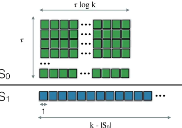
We observe in 2.3b that after some number of rounds the sampling is focused around the maximum. At every time step, GP-UCB selects a point with the highest upper confidence bound. We show some intermediate steps in 2.3c– 2.3k. 15 2.4 Illustration of the solution setS=S0∪S1returned by the OSU algorithm. Each
square represents a single element of the solution set (kelements in total), and each row corresponds to the elements selected in a single run of GREEDY. In the firstτ runs of GREEDY, each solution is of sizeτlogk; the union of the selected elements corresponds to the setS0. Finally, in the last run of GREEDY, which corresponds toS1, the solution is of sizek− |S0|. . . 26 3.1 An illustration of TRUVAR. In 3.1a, 3.1b, and 3.1c, three points within the set
of potential maximizersMtare selected in order to bring the confidence bounds
to within the target range, and Mt shrinks during this process. In 3.1d, the
target confidence width shrinks as a result of the last selected point bringing the confidence withinMtto within the previous target. . . 30
List of Figures
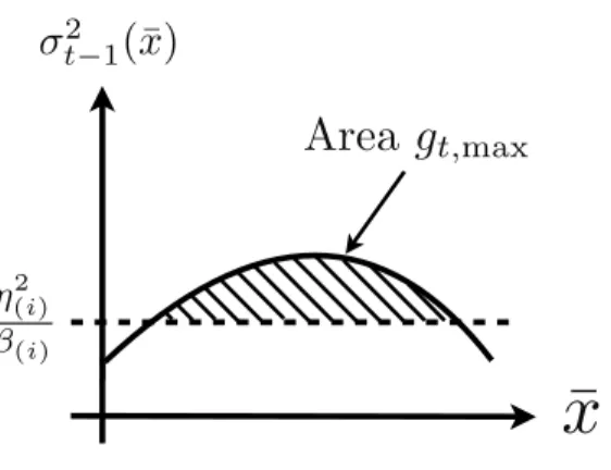
3.2 Illustration of the excess variancegt,max. . . 36 3.3 Experimental results for level-set estimation. . . 45 3.4 (a) Function used in synthetic level-set estimation experiments; (b) The amount
of cost used by TRUVAR for each of the three noise levels.. . . 46 3.5 Experimental results for Bayesian optimization. . . 47 4.1 (a) A functionf and its maximizerx∗0; (b) for= 0.06andd(x,x) =|x−x|,
the decision that corresponds to the local “wider” maximum off is theoptimal -stabledecision; (c) GP-UCB selects a point that nearly maximizesf, but is strictly suboptimal in the-stable sense. . . 57 4.2 An execution of STABLEOPTon the running example. Figures 4.2a and 4.2b
give an example of the selection procedure of STABLEOPTat two different time steps. We observe that aftert= 15steps,x˜tobtained in Eq. 4.8 corresponds to
x∗. The intermediate steps are presented in the subsequent rows. . . 61
4.3 Synthetic function from [BNT10b] (in (a)), counterpart with worst-case perturba-tions (in (b)), and the performance (in (c)). STABLEOPTsignificantly outperforms the baselines. . . 67 4.4 Experiment on the Zürich lake dataset; In the later rounds STABLEOPT is the
only method that reports a near-optimal-stable point. . . 68 4.5 Robust robot pushing experiment (Left) and MovieLens-100K experiment (Right) 69 4.6 Illustration of functionsf1, . . . , f5equal to a common function shifted by various
multiples of a given parameterw. In the-stable setting, there is a wide region (shown in gray for the dark blue curvef3) within which the perturbed function value equals−2η. . . 72 5.1 Examples of GP functions when= 0.01: (Left) SE kernel (l= 0.2); (Right)
Matérn kernel (ν = 1.5). Note that the location of the maximum changes significantly at distant times. . . 80 5.2 Numerical performance of upper confidence bound algorithms on synthetic data. 88 5.3 Numerical performance of upper confidence bound algorithms on real data. . . 90 6.1 Illustration of the setS=S0∪S1returned by PRO. The size of|S1|isk− |S0|,
and the size of|S0|is given in Prop 6.2.1. Every partition inS0 contains the same number of elements (up to rounding). . . 110 6.2 Numerical comparisons of the algorithms PRO-GREEDY, GREEDYand OSU,
and their objective values PRO-OA, OSU-OA and GREEDY-OA onceτ ele-ments are removed. Figure (i) shows the performance on the larger scale experi-ment where both GREEDYand STOCHASTIC-GREEDYare used as subroutines in PRO. . . 116 7.1 Approximation guarantee obtained in Remark 2. The green cross represents the
approximation guarantee whenf is submodular (γ =θ= 1). . . 138 7.2 Comparison of the algorithms on the linear regression task. . . 142
List of Figures
7.3 Logistic regression task with synthetic dataset. . . 143 7.4 Logistic regression with MNIST dataset. . . 144 7.5 Comparison of the algorithms on the variance reduction task. . . 145
List of Tables
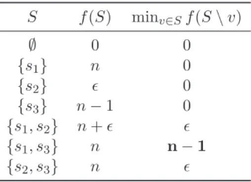
2.1 Bayesian and non-Bayesian settings and their correponding assumptions. The kernel functionkis typically assumed to be known in both settings. . . 20 2.2 Functionf used to demonstrate that GREEDYcan perform arbitrarily badly. . . 24 3.1 Summary of simple regret bounds for a fixed RKHS norm boundBand noise
levelσ2. . . . 41 6.1 Algorithms for robust monotone submodular optimization with a cardinality
constraint. Our algorithm PRO-GREEDY is efficient and allows for greater robustness. . . 106 6.2 Datasets and corresponding objective functions. . . 114
List of Algorithms
1 Bayesian Optimization Pseudocode . . . 14
2 GP-UCB [SKKS10] . . . 16
3 Truncated Variance Reduction (TRUVAR) for Bayesian Optimization [BSKC16] 31 4 BO Parameter Updates for TRUVAR [BSKC16] . . . 31
5 Truncated Variance Reduction (TRUVAR) for Level-Set Estimation [BSKC16] 33 6 LSE Parameter Updates for TRUVAR [BSKC16] . . . 33
7 STABLEOPT[BSJC18] . . . 60
8 GP-UCB with Resetting (R-GP-UCB) [BSC16] . . . 83
9 Time-Varying GP-UCB (TV-GP-UCB) [BSC16] . . . 84
10 Partitioned Robust Submodular optimization algorithm (PRO) [BMSC17b] . . 109
Bibliographic Note
This dissertation is based on the following publications:
• Ilija Bogunovic, Jonathan Scarlett and Volkan Cevher. "Time-Varying Gaussian Process Bandit Optimization". International Conference on Artificial Intelligence and Statistics
(AISTATS), 2016 [BSC16].
• Ilija Bogunovic, Jonathan Scarlett, Andreas Krause and Volkan Cevher. "Truncated Vari-ance Reduction: A Unified Approach to Bayesian Optimization and Level-Set Estimation".
Conference on Neural Information Processing Systems(NIPS), 2016 [BSKC16].
• Ilija Bogunovic, Slobodan Mitrovic, Jonathan Scarlett and Volkan Cevher. "Robust Sub-modular Maximization: A Non-Uniform Partitioning Approach".International Conference on Machine Learning (ICML), 2017 [BMSC17b].
• Ilija Bogunovic*, Junyao Zhao* and Volkan Cevher. "Robust Maximization of Non-Submodular Objectives".International Conference on Artificial Intelligence and Statistics
(AISTATS), 2018 [BZC18].
• Ilija Bogunovic, Jonathan Scarlett, Stefanie Jegelka and Volkan Cevher. "Adversarially Robust Optimization with Gaussian Processes". Accepted toConference on Neural Infor-mation Processing Systems(NIPS), 2018 [BSJC18].
Other publications relevant to this disseration are:
• Ilija Bogunovic, Volkan Cevher, Jarvis Haupt and Jonathan Scarlett. "Active Learning of Self-concordant like Multi-index Functions".International Conference on Acoustics, Speech and Signal Processing(ICASSP), 2015 [BCHS15].
• Luca Baldassarre, Yen-Huan Li, Jonathan Scarlett, Baran Gözcü, Ilija Bogunovic and Volkan Cevher. "Learning-Based Compressive Subsampling".IEEE Journal on Selected Topics in Signal Processing, 2016 [BLS+16].
• Ashkan Norouzi Fard, A. Bazzi, Marwa El Halabi, Ilija Bogunovic, Ya-Ping Hsieh and Volkan Cevher. "An Efficient Streaming Algorithm for the Submodular Cover Problem".
Chapter 0. Bibliographic Note
• Jonathan Scarlett, Ilija Bogunovic and Volkan Cevher. "Lower Bounds on Regret for Noisy Gaussian Process Bandit Optimization". Conference on Learning Theory(COLT), 2017 [SBC17].
• Ilija Bogunovic, Slobodan Mitrovic, Jonathan Scarlett and Volkan Cevher. "A Distributed Algorithm for Partitioned Robust Submodular Maximization". Inter. Workshop on Compu-tational Advances in Multi-Sensor Adaptive Processing (CAMSAP), 2017 [BMSC17a]. • Slobodan Mitrovic, Ilija Bogunovic, Ashkan Norouzi Fard, Jakub Tarnawski and Volkan
Cevher. "Streaming Robust Submodular Maximization: A Partitioned Thresholding Ap-proach".Conference on Neural Information Processing Systems(NIPS), 2017 [MBNF+17]. • Paul Rolland, Jonathan Scarlett, Ilija Bogunovic and Volkan Cevher. "High Dimensional
Bayesian Optimization via Additive Models with Overlapping Groups". International Conference on Artificial Intelligence and Statistics(AISTATS), 2018 [RSBC18].
1
Introduction
The past years have witnessed significant progress in technologies that are based on data-driven systems that interact with the environment, acquire information, reason and make decisions. Recent technological advances include the developments of the first program to defeat a Go world champion [SSS+17], agile robots that can learn complex behavior and operate in non-trivial environments [HSL+17] and systems for adaptive data center management that reduce energy costs [EG16], to name a few. Decision-making for self-driving cars has also generated significant improvement in various operative capabilities following in several prototypes already driving on our roads and streets [SAMR18]. In online advertising and recommendation systems, interactive machine learning systems are used to automatically generate a personalized recommendation to a user from a large pool of possibilities. Based on the users’ feedback, these systems can integrate and utilize the newly acquired information and provide better recommendations for future interactions. Similar machine learning systems with human feedback are also used to infer what humans want, e.g., by being informed which of two proposed responses is preferred [CLB+17].
Interactive data-driven systems are also beginning to be introduced into other fields, e.g., medicine, astronomy, computational biology, chemistry, etc. New applications usually appear with more complex requirements, specific types of constraints, as well as ever-growing decision spaces. For instance, in chemical design, we seek to discover molecules that have some desirable properties, and which can be the key to the discovery of a new drug or material. However, the number of molecules with potential medical properties is enormous – estimated to be in between1023and1060[GBWD+18]. An additional challenge is the fact that decisions are usually
costly(e.g., testing a new chemical compound requires running expensive simulations) while the resulting observations can often benoisy(e.g., the outcome of running the same experiment might vary). A significant challenge is how to automate the exploration of such and similar spaces and locate promising candidates quickly. Fortunately, the design space in many real-world problems is oftenstructured, e.g., it is usually the case that similar molecules will have similar properties and similar movies will be rated similarly by the user. Hence, the key to tackling such problems lies in the ability of the systems toadaptivelymake decisions based on the previous observations and current model, with the goal of reducing the number of expensive interactions.
Chapter 1. Introduction
The greater need for adaptive data-driven systems that can perform in the real world tasks has also introduced important additional requirements. When it comes to a significant number of relevant techonologies, one of the requirements that is in focus is robustness. Failures, unpredictable or unstable performance of such systems can often lead to considerable social and economic consequences [Rec18]. As a result, it is important for the decisions they made to be robust in the case of adversarial attacks, dynamic effects and temporal variations, parameter perturbations, a mismatch between simulations and reality, etc. In various practical applications it is beneficial to go beyond a single best decision, but discover multiple sufficiently good backup solutions in the case of some of them result in failure. An essential question in all of these settings is how to make robust decisions while still being able to guarantee strong theoretical performance for our methods. In this dissertation, we study and address this general challenge by considering specific tasks and problem formulations.
The central task in many interactive machine learning systems can often be formalized as the iterative optimization of the unknownblack-boxfunction that represents some quantity of interest. The only way to learn about the unknown objective is throughbanditfeedback, i.e., point evaluations. For example, in recommender systems, the user’s preferences are unknown, and we learn about them by iteratively recommending items and observing the feedback; in automatic chemical design, we regularly select molecules for testing, and we learn about their properties by querying the expert or by running specific simulations. Decision making in these settings corresponds to either adaptive experimentation with the goal of finding the best design, or balancing betweenexploration(i.e., acquiring new information about the unknown quantity) andexploitation(i.e., making decisions that are believed to be the best based on the previous interactions) with the goal of cumulative maximization of the importance of choices.
As mentioned before, we can benefit from the fact that the design space is structured in many real-world applications. A way to exploit this is to take the Bayesian perspective and assume a prior model of the unknown function. Typically, a Gaussian process (GP)[RW06] is used as a model when the central assumption is that adjacent observations should reveal information about each other [SS98]. In this dissertation, we considerBayesian optimization (BO) – a powerful model-based framework for adaptive experimentation, where the primary goal is the optimization of the unknown function via sequentially chosen decisions and ob-servations. Since its introduction, BO has been applied in different fields, e.g., recommender systems [VNDBK14], robotics [LWBS07], control and reinforcement learning [BSK16], environ-mental monitoring [SKKS10], preference learning [GDDL], combinatorial optimization [BP18] and many others. Perhaps, the most famous application is automatic hyperparameter tuning in machine learning, where BO is used to automatically select the best model and its associated hyperparameters [SLA12]. A great number of methods for BO (i.e. selection strategies that utilize the model to guide the sequential search) have been developed over time [SSW+16]. One popular algorithm is GP-UCB [SKKS10], which builds confidence bounds around the unknown function and uses theupper confidence bound criterion to select its next decision. This idea comes from the seminal work [LR85] on the multi-armed bandit problem, where this strategy is used to balance between exploration and exploitation.
1.1. Contributions
Despite a significant number of methods for Bayesian optimization and experimentation, numerous challenges remain. How can we perform adaptive experimentation in search for a design that not only maximizes the unknown quantity but is also robust againstadversarial perturbations? How can one perform adaptive decision making to discover all"sufficiently good"design choices instead of finding a single best solution alone? In many of the applications, the unknown quantity is not static, but it varies with time. Besides the standard decision making dilemma of exploration vs. exploitation, how can we further balance betweenforgettingvs.rememberingof the acquired data? Furthermore, how shall we choose which experiments to run (i.e., where to evaluate the unknown function) in the case ofpoint-wise costsandheteroscedastic noise(i.e., when querying the unknown function at different points in the decision space leads to different costs and amount of noise in observations)? How can we automatically choose experiments in arobustway in the case some of them fail? These are some of the research questions that we consider in this dissertation with the goal of enhancing both robust and adaptive decision making in BO and related methods. Under most of these challenges, the standard BO methods become inadequate. To tackle these questions, we propose variousconfdience-boundbased algorithms that, despite the lack of knowledge of the actual underlying function, are able to make decisions based on the previous interactions and their confidence in the model.
Finally, in many real-world tasks, it is of interest to choose a set of decisions in every interaction. However, what if some of the selected decisions/experiments fail? In many situations, we do not have a reasonable prior distribution on how failures happen, or we require robustness guarantees with a high level of certainty. In such case, protecting against worst-case failures is essential. In this dissertation, we address this question by formalizing it as the combinatorial optimization problem in which the goal is to choose a set of decisions (from a potentially large pool) that maximize some objective value so that if some decisions result in failure, the value degrades as little as possible. Finding a robust set of choices is not only of interest in adaptive experimentation and the case when experiments can fail, but it can be essential in many important machine learning applications. Some of the relevant problems where it is useful to select a robust set of decisions include feature selection [KED+17], influence maximization [KKT03], sensor placement [KSG08], data summarization [Mir17], when interpreting machine learning models [RSG16], just to name a few. In many of these, the objective set function satisfies the natural notion of diminishing returns –submodularity. In such cases and when decisions can fail, the standard greedy algorithm [NW78] that is near-optimal in the non-robust setting can perform arbitrarily badly. In this dissertation, we propose efficient algorithms for robust decision selection that address this issue by exploiting a very simple idea: The key is to select decisions that will admit a large objective value, but also a right number of redundant decisions that can"cover for"
the important ones in the case they fail.
1.1
Contributions
In this dissertation, we explore four research challenges related to robust and adaptive decision making, with a particular focus on algorithms that provide strong theoretical guarantees:
Chapter 1. Introduction
f
f(x∗)
(a) Unknown functionf and its maximizerx∗
h
(b) Level sets
Figure 1.1: In BO the goal is to findx∗alone (Figure 1.1a), while in LSE (Figure 1.1b) one seeks to find all "sufficiently good" points, i.e., points for whichf(x)is above the given thresholdh.
1. Designing a versatile and cost-effective method for Bayesian optimization and level-set estimation.
Bayesian optimization (BO) and level-set estimation (LSE) are related problems that are typically studied in isolation. Bayesian optimization [SSW+16] provides a powerful framework for automating experimentation and finds applications in robotics, environmental monitoring, and automated machine learning, etc. One seeks to find the maximum of anunknownreward function that is expensive to evaluate, based on a sequence of suitably-chosen decisions and their noisy observations. Level-set estimation (LSE) [GCHK13] is closely related to BO, but instead of seeking a maximizer, one seeks to classify the domain into points that lie above or below a certain threshold. Finding the best solution alone, as is the case in BO, might not be sufficient in applications whererobustnessordiversityof solutions is required. In such cases, LSE can be used to find all “sufficiently good” solutions (see Figure 1.1 for an illustration).
Popular methods for BO include expected improvement (EI), probability of improvement (PI), and Gaussian process upper confidence bound (GP-UCB) [SSW+16, SKKS10]. An algorithm for level-set estimation with GPs is given in [GCHK13], which keeps track of a set of unclassified points. These algorithms have theoretical guarantees and good computational complexity, but due to theirmyopicnature in considering no more than a single step into the future, it is unclear how to incorporatepointwise costs(i.e., a scenario in which different sampling locations are associated with different costs) and several other settings. In contrast, so-calledone-step lookaheadBO methods, entropy search (ES) [HS12], its predictive version (PES) [HLHG14] and minimum regret search (MRS) [Met16] permit versatility with respect to costs [SSA13], heteroscedastic noise [GWB97], and multi-task scenarios [SSA13]. Unlike the myopic algorithms, these are computationally expensive and, to our knowledge, no theoretical guarantees have been provided for these one-step lookahead algorithms. Hence, we seek to design a versatile, computationally efficient and cost-effective algorithm with rigorous theoretical guarantees.
In Chapter 3, we present an algorithm, truncated variance reduction (TRUVAR), that addresses Bayesian optimization and level-set estimation with Gaussian processes in aunified fashion.
1.1. Contributions
f(x∗0) f(x∗)
f
(a) Unknown functionf
min
δ∈Δ(x)
f(x+δ)
(b) Robust objective
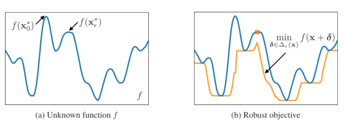
Figure 1.2: (a) A functionf and its maximizerx∗0; (b) for the adversarial budget= 0.06and distance functiond(x,x) = |x−x|, the decisionx∗ that corresponds to the local “wider” maximum off is theoptimal-stabledecision.
The algorithm greedily shrinks the total variance, up to a truncation threshold, within a set of potential maximizers (BO) or unclassified points (LSE), which is updated based on confidence bounds. TRUVAR is effective in important settings that are typically non-trivial to incorporate into the standard myopic algorithms, such as pointwise costs and heteroscedastic noise. On the other hand, compared to the one-step lookahead algorithms for BO, TRUVAR avoids the computationally expensive task of averaging over the posterior and/or measurements, and comes with rigorous theoretical guarantees for the two settings. Moreover, we present a new result in themulti-fidelitysetting where, while sampling, one can select from a number of noise levels having associated costs. The cost-effectiveness of TRUVAR is demonstrated on both synthetic and real-world data sets, where it is able to outperform the competitor methods while incurring a significantly smaller sampling cost.
2. Designing a method for robust Bayesian optimization.
In many applications in which the goal is to optimize a black-box function, one is faced with forms of uncertainty that are not accounted for by standard algorithms. In robotics, the optimization is often performed via simulations, creating a mismatch between the model and the true function; in parameter tuning, the function is similarly mismatched due to limited training data; in recommendation systems, the underlying function is inherently time-varying, so the returned solution may become increasingly stale over time; the list goes on. We address these considerations by studying GP optimization with an additional requirement ofrobustness: The returned point may be perturbed by an adversary, and we require the function value to remain as high as possible even after this perturbation. This problem is of interest not only for attaining improved robustness to uncertainty but also for other related max-min optimization settings.
In general, for a given fixed perturbation budget, the function value of the global maximum after being adversarially perturbed might degrade significantly. We refer to the point that has the highest function value after being adversarially perturbed (in the worst-case sense) asstableoptimal (see Figure 1.2). In such setting, all the BO strategies (e.g., [HS12, WJ17, SJ17a, RMGO18]) whose goal is to identify the global non-robust maximum can become inherently suboptimal.
Chapter 1. Introduction 0 0.5 1 −2 −1 0 1 2 3 x ft ( x ) t = 200 t = 100 t = 10 t = 1 0 0.5 1 −4 −2 0 2 4 x ft ( x ) t = 200 t = 1 t = 10 t = 100
Figure 1.3: Two examples of time-varying reward functions. The location of the global maximum changes significantly at distant times.
In Chapter 4, we introduce a variant of GP optimization in which the returned solution is required to exhibit stability/robustness to an adversarial perturbation. We demonstrate the failures of standard BO algorithms, and we introduce a new algorithm STABLEOPT that overcomes these limitations. The algorithm is based on two distinct principles: optimism in the face of uncertainty when it comes to selecting where to sample next, and pessimism in the face of uncertaintywhen it comes to anticipating the perturbation of the selected point. We provide a novel theoretical analysis characterizing the number of samples required for STABLEOPTto attain anear-optimal robustsolution, and we complement this with an algorithm-independent lower bound. We provide several important variations of our max-min optimization framework and theory, including the classical robust formulation, robust estimation, and group identification problems. We experimentally demonstrate a variety of potential applications of interest on real-world data sets, and we show that STABLEOPTconsistently succeeds in finding astable maximizerwhere several BO and baseline methods fail.
3. Can we design "no-regret" methods in the case of time-varying rewards?
In the previous two research challenges, the unknown objective function was assumed to be time-invariant, i.e., it wasstaticand did not vary with time. However, in many practical appli-cations, the function to be optimized varies with time: In sensor networks, measured quantities such as temperature undergo fluctuations; in recommender systems, the users’ preferences may change according to external factors; similarly, financial markets are highly dynamic. Studying time-varying effects is of great importance in such applications.
In the time-invariant setting (i.e., classical setting), several different algorithms are known to be
"no-regret"(e.g., [SKKS10]). Simply put, for a sufficiently large time horizon, these algorithms are guaranteed to find the global maximum. However, in the case of time-varying reward functions, the maximum function value and its location could change drastically throughout the time horizon. In such cases, the performance of these standard Bayesian optimization algorithms may deteriorate, since these continue to treat stale data as being equally important as fresh data.
1.1. Contributions
Balancing between exploration and exploitation is not sufficient, and leads to the non-vanishing regret performance of the standard algorithms. This initiates the study of the additional forgetting-remembering dilemma and the development of algorithms that can exploit both spatial and temporal correlations present in the reward function.
In Chapter 5, we take a novel approach to handling time variations, modeling the reward function as a Gaussian process (GP) that varies according to a simple Markov model (as shown in Figure 1.3). We prove that no algorithm can attain vanishing regret for any fixed function variation rate. This motivates the study on how the regretjointlydepends on the time horizon and the rate at which the reward function varies. We develop two algorithms based on the upper confidence bound strategy. The first, R-GP-UCB, completely forgets about the past data at regular intervals. The second, TV-GP-UCB, instead forgets about old data in a smooth fashion. Our main contribution comprises of novel regret bounds for these algorithms, providing an explicit characterization of the trade-off between the time horizon and the rate at which the function varies. We test the performance of the algorithms on both synthetic and real data and show that R-GP-UCB is computationally more efficient while the gradual forgetting of TV-GP-UCB performs favorably compared to the sharp resetting of R-GP-UCB. Moreover, both algorithms significantly outperform the standard BO algorithms, since they treat stale and fresh data equally.
4. How can we efficiently select a robust set of experiments/decisions that maximize our objective of interest, such that it degrades as little as possible if some of them fail?
In all the previous challenges, we considered the task of sequentially optimizing an unknown function from point evaluations that require performing costly experiments. When a batch of points is to be selected, this becomes the problem of subset selection, which we need to solve in every round. In case that experiments can fail, protecting against worst-case failures of expensive trials is of great importance. This challenge is not only associated with the robust experimentation, but it also arises in other important machine learning applications where the goal is to select a robust set of items that maximize some objective of interest. For instance, (i) in influence maximization problems, a subset of the chosen users may decide not to spread the word about a product; (ii) in summarization problems, a user may decide to remove some items from the summary due to their personal preferences; (iii) in the problem of sensor placement for outbreak detection, some of the sensors might fail; (iv) in the problem of feature selection, some selected features might be missing at the test time. In situations where one does not have a reasonable prior distribution on the elements removed, or where one requires robustness guarantees with a high level of certainty, protection against worst-case removals becomes essential.
The problem can be formalized as the robust set selection problem in which we want to select a set of items of sizekto maximize some objective function such that the utility of the selected set degrades as little as possible after the worst-case adversarial failure (i.e., removal) ofτ of them. We consider both the case when the objective function satisfies the natural notion of diminishing returns (i.e., adding an item to a set is "more beneficial" if it is done earlier than later in the selection process) –submodularity[KG12], and the case ofnon-submodularobjectives [DK08].
Chapter 1. Introduction
We address the former case in Chapter 6. A constant-factor approximation guarantee was given in [OSU16] when the allowed number of removals isτ =o(√k). We solve a key open problem raised therein, presenting a new and efficient Partitioned Robust (PRO) submodular maximization algorithm that achieves the same constant factor guarantee for more generalτ = o(k). Our algorithm constructs partitions consisting of buckets with exponentially increasing sizes, and applies standard submodular optimization subroutines on the buckets to construct the robust solution. We numerically demonstrate the performance of PROin data summarization [Mir17] and influence maximization [KKT03] tasks, demonstrating gains over both the non-robust greedy algorithm [NW78] and the algorithm of [OSU16].
We consider the case of non-submodular objectives in Chapter 7. We propose a simple and practical algorithm OBLIVIOUS-GREEDY, and prove the first constant-factor approximation guarantees for a broader class of non-submodular objectives. The obtained theoretical bounds also hold in the linear regime, i.e., when the number of allowed removals τ is linear in k. Our bounds depend on a few parameters includingsubmodularity ratioandinverse curvature, that essentially, characterize how close the objective is to being submodular and approximate diminishing returns property of the objective, respectively. We provide a summary of these and other useful parameters that can be used to characterize any monotone set function, and prove some interesting relations between them.
The obtained relations allow us to provide bounds for these parameters for two important non-submodular objectives including the variance reduction objective and the one used in sparse support/feature selection problems. The variance reduction objective is the one used in the TRUVAR rule (introduced in Challenge 1). While this objective is not submodular in general, we show that constant factor guarantees can still be obtained and OBLIVIOUS-GREEDYcan be used at every round in Bayesian optimization to select a robust set of experiments efficiently. By considering the sparse feature selection problem, we provide a novel connection betweenstrong convexityandweak supermodularity(i.e., the property that tells how close the objective is to being supermodular). This result complements the one from [EKDN16] where the same connection is shown between strong convexity andweak submodularity. This result can potentially enlarge the number of applications where supermodular optimization and algorithms can be used. Finally, we empirically demonstrate the robust performance of our algorithm by considering these objectives. On various datasets, OBLIVIOUS-GREEDYconsistently outperforms both robust and non-robust algorithms in terms of the robust objective value, but also when it comes to the generalization performance (in the feature selection problem) in the case of unseen data.
1.2. Organization of the Thesis
1.2
Organization of the Thesis
The structure of this dissertation is as follows:• In Chapter 2, we provide a brief introduction to Bayesian optimization. We review the GP-UCB algorithm [SKKS10] and relevant theoretical results in BO. We proceed with a short review on submodular functions and optimization. Finally, we focus on a specific problem in robust submodular optimization and consider the previous work and algorithms. • In Chapter 3, we study the unified and cost-effective approach to BO and LSE. We propose
a new algorithm TRUVAR and investigate its theoretical guarantees both in BO and LSE. Other settings and their corresponding theoretical guarantees are also considered, including pointwise costs, heteroscedastic noise, multi-fidelity, and the non-Bayesian setting. • In Chapter 4, we introduce the problem of adversarially robust Gaussian process
optimiza-tion and propose a novel robust algorithm STABLEOPT. We study both theoretical and empirical performance of our algorithm in this and other robust settings including robust Bayesian optimization, robustness to unknown parameters, and group identification. • In Chapter 5, we consider the problem of Gaussian process optimization when the unknown
function varies with time. We propose new algorithms TV-GP-UCB and R-GP-UCB that can penalize the old data and study the setting-specific lower and upper regret bounds that jointly depend on the time horizon and rate of variation.
• In Chapter 6, we investigate the problem of robust submodular maximization in the presence of adversarial removals. We propose a novel robust algorithm PRO-GREEDYand address a key question from [OSU16], that is, whether the constant factor approximation guarantee therein can hold in the case of a greater number of allowed removals.
• In Chapter 7, we study the same problem as in Chapter 6 in the case when the objective is non-submodular. We present OBLIVIOUS-GREEDY and analyze its approximation guarantees in terms of the parameters that characterize set functions (e.g., submodularity ratio). We investigate the bounds for these parameters in different important applications. • In Chapter 8, we review the main contributions of each chapter in this disseration, and
provide various directions for future research.
We begin Chapters 3-7 by formally stating the considered problem followed by the main algorithm, theoretical results and experimental evaluations. Chapter-specific related work and main contributions are listed at the beginning of every chapter. In Chapters 3-7, we provide most of the proofs in the subappendices at the end of each chapter.
Chapter 1. Introduction
1.3
Notation
In this section, we outline definitions of the most commonly-used mathematical symbols in this disseration.
We useRto denote the set of real numbers, andR+to denote the set of positive real numbers. The set of natural numbers is denoted byN, the set of positive natural numbers byN+, and the set of integers byZ.
We use bold symbols for vectors and matrices, with the latter being capitalized, e.g.,aandA. To denotei-th entry of a vector we use subscriptai. We denote the transposes ofaandAbyaT
andAT, and ifAis invertible, its inverse is denoted byA−1. The Euclidean norm of a vector
ais denoted bya2, the sum of the absolute values of its entries bya1, and the maximum absolute value of its entries bya∞. For a squaren×nmatrixA, we usedet(A)to denote its determinant and tr(A)to denote its trace. We useInto denote identity matrix of sizen×n. For
a vectora, we writediag(a)for a diagonal matrix containing the elements of vectoraon the main diagonal. The inner product of two vectors is denoted with·,·. For two matricesAand
Bof sizen×n, the Hadamard productA◦Bresults in a matrixC of sizen×n, with elements given byCi,j = (A)i,j(B)i,j. For a matrixA, we useAF to denote its Frobenius norm.
Letf(·)andg(·)be two functions defined on some unbounded subset of the real numbers. We write f(x) = O(g(x)) if |f(x)| ≤ C|g(x)| for some C and sufficiently large x, and
f(x) = o(g(x))if g(x) = 0and limx→∞ fg((xx)) = 0. Similarly, we write f(x) = Ω(g(x))if
|f(x)| ≥C|g(x)|for someCand sufficiently largex. We similarly use the notationO∗(·),Ω∗(·) to denote asymptotics up to logarithmic factors.
The symbol∼means "distributed according to". We use P[·]to denote the probability of an event. The indicator function of an eventE is denoted by1E. E[·]andVar[·]are used for
the expectation and variance of a random variable when the probability distribution is obvious from the context, and Eq(x)[f(x)],Varq(x)[f(x)]whenx ∼ q(x). Et[·]is used to denote the
expectation of a random variable with respect to its posterior distribution at time t. We use
H(X) to denote entropy, H(X|Y) for conditional entropy, I(X;Y) for mutual information andD(P||Q)for KL divergence. We useΦto denote standard normal CDF. We writeGPto denote a Gaussian process distribution andf ∼GP(μ(x), k(x,x))to denote that functionf is distributed according to a Gaussian process with meanμ(·)and kernel functionsk(·,·). After observingtdata points, we useμt(·)andσt2(·)to denote the posterior mean and variance of a
GP, and we useKtto denote the kernel matrix fortnoiseless observations.
For a setA, we write |A|to denote its cardinality, and 2A to denote its power set. For a function f defined on sets, f(A|B) denotes the marginal gain of adding set A to set B, i.e.
f(A∪B)−f(B). We useA\Bto denote set difference. For an integerk >0, we write[k]for the set{1,· · ·, k}. The floor and ceiling functions are denoted by·and·, respectively. For a vectora, we write supp(a)for the set{i:xi= 0}, anda0 for|supp(a)|.
2
Background Material
In this chapter, we present an overview of Gaussian process (GP) models that are frequently used in Bayesian optimization (BO). Various methods for adaptive experimentation are discussed together with the most common performance metrics. We provide a summary of the existing theoretical results in BO that are most relevant to the work presented in the subsequent chapters of this dissertation. In the second part of this chapter, we provide a short review of submodular functions and the relevant results in submodular optimization. Finally, we discuss the robust submodular formulation in which we need to choose a set of decisions under uncertainty that some of them might result in failure.
2.1
Gaussian Processes (GPs)
In this section, we provide a brief overview of Gaussian process models. A more comprehensive introduction can be found in [RW06, Section 2].
A Gaussian process over some input spaceDis a collection of dependent random variables {f(x)}x∈Dsuch that every finite subset of these random variables{f(xi)}ni=1,n∈Nis jointly Gaussian. Any GP is fully specified by its meanμ:D→Rand kernel (covariance) function
k:D×D→R, and hence it is denoted byGP(μ(·), k(·,·)). Because GPs define a distribution over functions, they are frequently used in nonparmetric and nonlinear regression to model an unknown function. Forf ∼ GP(μ(·), k(·,·)), we havef : D→ Randf(x) is Gaussian for everyx∈D, with meanμ(x) =E[f(x)]and variancek(x,x) =E[(f(x)−μ(x))2].
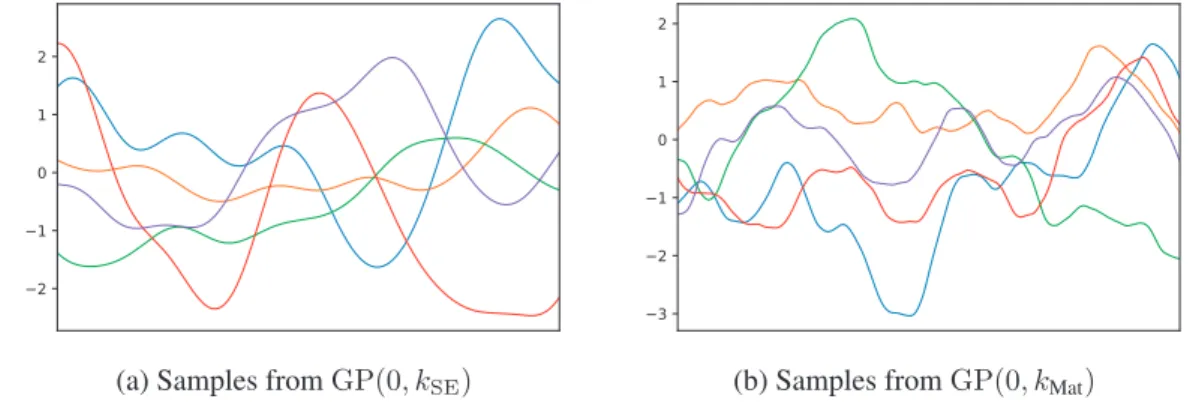
Typically, we use GPs as a prior model when the main assumption is that the function values of nearby inputs should reveal information about each other [SS98]. We can model versatile classes of functions by using different kernel functions (see Figure 2.1). An important class of kernels is the class ofstationary kernels. These kernels are translation invariant, meaning that the dependence onx,xis only through their difference, i.e.,k(x,x) =k(τ)forτ =x−x.
Chapter 2. Background Material
(a) Samples fromGP(0, kSE) (b) Samples fromGP(0, kMat)
Figure 2.1: Example of functions sampled from zero mean GP with SE and Matérn kernel. Different kernel functions can be used to model versatile classes of functions.
Two of the most commonly used stationary kernels in practice are squared exponential (SE)1and Matérn kernels: kSE(x,x) = exp −x−x2 2l2 , (2.1) kMat(x,x) = 21−ν Γ(ν) √2νx−x l Jν √2νx−x l , (2.2)
whereldenotes the length-scale,ν >0is an additional parameter that dictates the smoothness (the smaller this parameter is, the rougher the sampled functions are) andJ(ν)andΓ(ν)denote the modified Bessel and Gamma functions, respectively ([RW06, Section 4.2.1]). Functions sampled from SE kernel are infinitely differentiable almost surely. In the case of the Matérn kernel, as its parameterν→ ∞we recover the SE kernel. An overview of other kernel functions that can be interesting in practical applications can be found in [Duv14, Chapter 2]. When it comes to the mean function a usual assumption is that it is zero everywhere [RW06, Section 2.7]. We useGP(0, k)to denote a zero mean GP with kernelk.
Supposef ∼GP(0, k), and suppose we samplef at{x1, . . . ,xt}and observe{y1, . . . , yt}
where for everyi∈[t]:
yi =f(xi) +zi and zi∼ N(0, σ2).
By the GP property, for anyx∈Dwith the corresponding valuef(x), it holdsyt= [y1, . . . , yt]T
andf(x)are jointly Gaussian given{x1, . . . ,xt}:
f(x) yt ∼ N 0, k(x,x) kt(x)T kt(x) Kt+σ2It , (2.3) Here,kt(x)T = k(x1,x), . . . , k(xt,x) andKt= k(xt,xt) t,t ∈R
t×tis the kernel matrix.
2.2. Bayesian Optimization
(a) Samples from prior (b) Samples from posterior (c) Posterior uncertainty
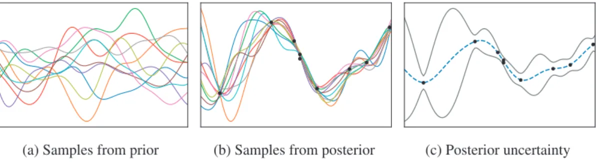
Figure 2.2: An illustration of Bayesian posterior updates in GPs. In (a), we show samples from the GP prior. After receiving some (noisy) observations (black circles), posterior samples are illustrated in (b). In (c), we show the posterior mean prediction (dashed curve) plus and minus its 3 standard deviations (both obtained via (2.4)). We observe that the uncertainty shrinks around the observed points and is larger further away from observations.
By using the formula for the conditional distribution associated with a jointly Gaussian random vector [RW06, Appendix A], one can show that conditioned on the observed data{(xi, yi)}ti=1, the posterior process is again GP with the posterior mean and variance:
μt(x) =kt(x)T Kt+σ2I −1 yt, σt2(x) =k(x,x)−kt(x)T Kt+σ2It −1 kt(x) (2.4)
Therefore, for everyx∈D, conditioned on{(xi, yi)}ti=1, the posterior distribution off(x)is Gaussian, i.e.,N(μt(x), σt2(x)). The Bayesian posterior mechanics are illustrated in Figure 2.2.
As can be observed in (2.4), the posterior mean and variance at some input can be computed analytically in closed form. This property, and together with the ability to describe uncertainty in the predictions, are the main reasons why GPs are frequently used in many machine learning applications. The algorithms and theory developed in later sections will heavily rely on these elegant features of GPs. In practice, Cholesky decomposition is used instead of directly inverting the kernel matrix in (2.4) (see Algorithm 2.1 in [RW06, Section 2.2] for more details).
2.2
Bayesian Optimization
Bayesian optimization (BO) refers to a sequential model-based approach for optimizing an
unknownand usuallymultimodalreward functionf :D→Rover some input spaceD, where a prior belief of the possible reward functions is prescribed. The unknown function is ablack-box, meaning that it can be only observed through so calledbandit feedback, i.e., point evaluations (no gradient information is available). We also assume that every function evaluation iscostly. Since its introduction, BO has successfully been applied to numerous applications, including robotics [LWBS07], algorithm parameter tuning [SLA12], recommender systems [VNDBK14], environmental monitoring [SKKS10], and many more.
Chapter 2. Background Material
Algorithm 1Bayesian Optimization Pseudocode 1: fort= 1,2, . . . do
2: choosextby optimizing some acquisition (i.e., auxiliary) functionϑ(·):
xt∈arg max
x ϑ
x;{xi, yi}ti−=11
3: observe the objective function sampleytatxt
4: augment data and update probabilistic model
The main idea in BO is to sequentially acquire data and refine the prescribed reward function model via Bayesian posterior updates. The overall procedure is given in Algorithm 1. We proceed by explaining the three main components: aprobabilistic model, anacquisition function(i.e., auxiliary function) and aperformance metric.
When it comes to the model, the most common option is to use a Gaussian process prior to model the unknown reward function, that is to assumef ∼GP(0, k). In practice, the parameters of the GP kernel function can be learned from the observed data via the marginal likelihood approach or sampling procedures (see [RW06, Section 5]). Given such model, the procedure develops in time steps (see Algorithm 1), where at every time stept, the unknown function is sampled at a pointxt, and the corresponding observationytis received. By aggregating a new
data pair(xt, yt), the model is updated via Bayesian posterior updates (outlined in (2.4)) by using
all the previously collected data{xi, yi}ti=1.
An acquisition functionϑ:D→ R, is a surrogate function that makes use of the posterior model to guide the sampling procedure. It is usually designed to balance betweenexplorationand
exploitation, i.e., it has high values where the uncertainty of the model is large (corresponding to exploration), and/or where the prediction of the model is high (exploitation). At every time step, the acquisition function is optimized and the resulting pointxtis the one wheref is sampled at.
Acquisition functions are usually multimodal and potentially non-trivial to optimize. The central assumption in BO is thatf is expensive and/or time-consuming to evaluate, so that the overhead that comes with the optimization of the acquisition function is significantly cheaper. For example, when tuning complex machine learning systems, one evaluation off might correspond to training the system for a single hyperparameter configuration on a huge dataset, which might require days to finish. On the other hand, acquisition functions are defined on the posterior model, and hence to optimize them we do not require additional evaluations off. An important practical aspect is the global optimization of the acquisition function when the domain is compact
D⊂Rd(in contrast, whenDis finite this task is easier). Various global optimization solvers are used for this problem in practice (see [SSW+16, V.B] for more details). We note that in most of the theoretical results in BO, it is assumed that the kernel function is perfectly known and that the auxiliary optimizer finds the global maximum of the acquisition function (some of these assumptions are relaxed in, e.g., [WdF14],[WSJF14] and [SJ17a]). For more details on the practical aspects of BO, we refer the reader to the survey [SSW+16].
2.2. Bayesian Optimization
(a)t= 5 (b)t= 31
(c)t= 6 (d)t= 7 (e)t= 8
(f)t= 9 (g)t= 10 (h)t= 11
(i)t= 12 (j)t= 13 (k)t= 14
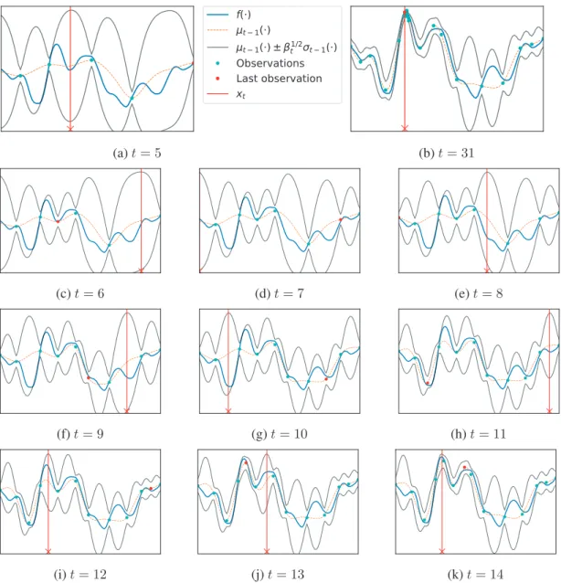
Figure 2.3: Demo run of GP-UCB: We start GP-UCB after5samples are collected (see 2.3a). We observe in 2.3b that after some number of rounds the sampling is focused around the maximum. At every time step, GP-UCB selects a point with the highest upper confidence bound. We show some intermediate steps in 2.3c– 2.3k.
Methods for BO
One of the most popular acquisition functions is based on the so-calledprinciple of optimism in the face of uncertainty. Simply put, despite the lack of knowledge in whatxis the best, the idea is to construct an optimistic guess as to how goodf(x)for everyx∈Dis and pickxwith the highest guess. This idea dates back to the seminal work [LR85] on the multi-armed bandit problem where theupper confidence bound criterionhas been used to balance between exploration and exploitation. Following the same approach, the Gaussian Process Upper Confidence Bound