Computer Science and Artificial Intelligence Laboratory
Technical Report
m a s s a c h u s e t t s i n s t i t u t e o f t e c h n o l o g y, c a m b r i d g e , m a 0 213 9 u s a — w w w. c s a i l . m i t . e d uMIT-CSAIL-TR-2006-078
November 27
, 200
6
Materialization Strategies in a
Column-Oriented DBMS
Daniel J. Abadi, Daniel S. Myers, David J. DeWitt,
and Samuel R. Madden
Materialization Strategies in a Column-Oriented DBMS
Daniel J. Abadi
Daniel S. Myers
David J. DeWitt
Samuel R. Madden
MIT
MIT
University of Wisconsin
MIT
[email protected]
[email protected]
[email protected]
[email protected]
Abstract
There has been a renewed interest in column-oriented database architectures in recent years. For read-mostly query workloads like those found in data warehouse and decision support applications, “column-stores” have been shown to perform particularly well rel-ative to “row-stores”. In order for column-stores to be readily adopted as a replacement for row-stores, they must maintain the same interface to external applications as do row-stores. This implies that column-stores must output row-store style tuples.
Thus, the input columns stored on disk must be converted to rows at some point in the query plan. The optimal point at which to
do this is not obvious. This problem can
be considered as the opposite of the
projec-tion problem in row-store systems. While
rows-stores need to determine where in query plans to place projection operators to make tuples narrower, column-stores need to deter-mine when to combine single-column projec-tions into wider tuples. This paper describes a variety of strategies for tuple construction and intermediate result representations, and then provides a systematic evaluation of these strategies.
1
Introduction
Vertical partitioning has long been recognized as a valuable tool for increasing the performance of read-intensive databases. Recent years have seen the emer-gence of several database systems that take this idea to the extreme by fully vertically partitioning database tables and storing them as columns on disk [16, 7, 11,
1, 10, 14, 13]. Research on these column-stores has
shown that for certain read-mostly workloads, this ap-proach can provide substantial performance benefits over traditional row-oriented database systems. Most column-stores choose to offer a standards-compliant relational database interface (e.g., ODBC, JDBC, etc.)
This means they must ultimately stitch together sepa-rate columns into tuples of data that are output. De-termining the tuple construction point in a query plan is the inverse of the problem of applying projections in a row-oriented database, since rather than deciding when to project an attribute out of an intermediate re-sult flowing through the query plan, the system must decide when to add it in. Lessons from when to ap-ply projection in row-oriented databases (projections are almost always performed as soon as an attribute is no longer needed) suggest a natural tuple construc-tion policy: at each point where a column is accessed, add the column to an intermediate tuple representa-tion if that column is needed by some later operator or is included in the set of output columns. Then, at the top of the query plan, these intermediate tuples can be directly output to the user. We call this process of adding columns to intermediate results materializa-tion, and call the simple scheme described aboveearly materialization, since it seeks to form intermediate tu-ples as early as possible.
Surprisingly, we have found that early materializa-tion is not always the best strategy to employ in a col-umn store. To illustrate why this is the case, consider a simple example: suppose a query consists of three selection operatorsσ1,σ2, andσ3over three columns,
R.a, R.b, and R.c (all sorted in the same order and stored in separate files), where σ1 is the most
selec-tive predicate and σ3 is the least selective. An early
materialization strategy could process this query as follows: Read in a block of R.a, a block of R.b, and
a block of R.c from disk. Stitch them together into
(likely more than one) block of row-store style triples (R.a, R.b, R.c). Applyσ1,σ2, andσ3in turn, allowing
tuples that match the predicate to pass through. However, there is another strategy that can be more efficient; we call this second approachlate materializa-tion, because it doesn’t form tuples until after some part of the plan has been processed. It works as fol-lows: first scan R.aand output the positions (ordinal offsets of values within the column) inR.athat satisfy the σ1 (these positions can take the form of ranges,
lists, or a bitmap). Repeat with R.b and R.c,
Next, use position-wise AND operations to intersect the position lists. Finally, re-accessR.a, R.b, andR.c
and extract the values of the records that satisfied all predicates and stitch these values together into output tuples. This late materialization approach can poten-tially be more CPU efficient because it requires fewer intermediate tuples to be stitched together (which is a relatively expensive operation as it can be thought of as a join on position) and position lists are a small, very compressible data structure that can be operated on directly with very little overhead. For example, 32 (or 64 depending on processor word size) positions can be intersected at once when ANDing together two po-sition lists represented as bit-strings. Note, however, that one problem of this late materialization approach is that it requires re-scanning the base columns to form tuples, which can be slow (though they are likely to still be in memory upon re-access if the query is prop-erly pipelined).
In this paper, we study the use of early and late materialization in the C-Store DBMS. We focus on
standard warehouse-style queries: read-only
work-loads, with selections, aggregations, and joins. We
study how different selectivities, compression tech-niques, and query plans affect the trade-offs in al-ternative materialization strategies. We run experi-ments to determine when one approach dominates the other, and develop an analytical model that can be used, for example, in a query optimizer to select a materialization strategy. Our results show that, on some workloads, late materialization can be an order of magnitude faster than early-materialization, while on other workloads, early-materialization outperforms late-materialization by an order of magnitude.
In the remainder of this paper we give a brief overview of the C-Store query executer in Section 1.1. We then detail the trade-offs between the two fun-damental materialization strategies in Section 2, and then present both pseudocode and an analytical model for some query plans using each strategy in Section 3. We then validate our models with experimental results by extending C-Store to support query execution us-ing any of the materialization strategies proposed in Section 4. We then describe related work in Section 5 and conclude in Section 6.
1.1 The C-Store Query Executor
We now provide a brief overview of the C-Store query executor, which is more fully described in [16, 3]
and available in an open source release [2]. The
components of the query executor relevant to the present study are the on-disk layout of data, the ac-cess methods provided for reading data from disk, the data structures provided for representing data in the DBMS, and the operators provided for manipulating these data.
Each column is stored in a separate file on disk as
a series of 64KB blocks and can be optionally encoded using a variety of compression techniques. In this pa-per we expa-periment with column-specific compression techniques (run-length encoding and bit-vector encod-ing), and with uncompressed columns. In a run-length encoded file, each block contains a series of RLE triples (V, S, L), where V is the value,S is the start position of the run, and Lis the length of the run.
A bit-vector encoded file representing a column of size n with k distinct values consists of k bit-strings of lengthn, one per unique value, stored sequentially. Bit-stringkhas a 1 in theithposition if the column it represents has the value kin theith position.
C-Store provides an access method (orDataSource)
for each encoding type. All C-Store data sources sup-port two basic operations: reading positions from a column and reading (position, value) pairs from a col-umn (note that any given instance of a data source can be used to read positions or (position, value) pairs, but not both). Additionally, all C-Store data sources ac-cept SARGable predicates [15] to restrict the set of results returned. In order to minimize CPU overhead, C-Store data sources and operators are block-oriented. Data sources return data from the underlying files in blocks of encoded data, wrapped inside a C++ class that provides iterator-style (hasNext() and getNext() methods) and vector-style [7] (asArray()) access to the data in the blocks.
In the Section 3.1 we will give pseudocode for three basic C-Store operators: DataSource (Select), AND, and Merge. We also describe the Join operator in sec-tion 4.3). The DataSource operator reads in a column of data and produces the column values that pass a predicate. AND accepts input position lists and pro-duces an output position list representing their inter-section. Finally, then-ary Merge operator combinesn
inputs of (position, value) pairs into a single output of
n-attribute tuples.
2
Materialization Strategy Trade-offs
In this section we present some of the trade-offs that are made between materialization strategies. A mate-rialization strategy needs to be in place whenever more than one attribute from any given relation is accessed (which is the case for most queries). Since a column-oriented DBMS stores each attribute independently, it must have some mechanism for stitching together multiple attributes from the same logical tuple into a physical tuple. Every proposed column-oriented archi-tecture accomplishes this by attaching either physical or virtual tuple identifiersor positionsto column val-ues. To reconstruct a tuple from multiple columns of a relation, the DBMS simply needs to find matching positions. Modern column-oriented systems [16, 6, 7] store columns in position order; i.e., to reconstruct the first tuple one needs to take the first value from each column, the second tuple is constructed from thesecond value from each column, and likewise as one iterates down through the columns. This accelerates the tuple reconstruction process.
As described in the introduction, tuple reconstruc-tion can occur at different points in a query plan. Early materializationconstructs tuples as soon as (or some-times before) tuple values are needed in the query plan. Late materialization constructs tuples as late as pos-sible, sometimes even at the query output. Each ap-proach has a set of advantages.
2.1 Late Materialization Advantages
Late materialization allows the executer to operate on positions and compressed, column-oriented data and defer tuple construction.
2.1.1 Operating on Positions
The process of tuple construction starts to get inter-esting as soon as predicates are applied to different columns. The result of predicate application are dif-ferent subsets of positions for difdif-ferent columns. Tuple reconstruction thus requires a equi-join on position of multiple columns. However, since columns are sorted by position, this join can be performed with a rela-tively fast merge join.
Positions can be represented using a variety of com-pression techniques. Runsof consecutive positions can be represented using position ranges of the form [start-pos, endpos]. Positions can also be represented as bit-maps using a single bit to represent every position in a column, with a ’1’ in the bit-map entry if the tuple at the position passed the predicate and a ’0’ otherwise. For example, for a position range of 11-20, a bit-vector of 0111010001 would indicate that positions 12, 13, 14, 16, and 20 contained values that passed the predicate. It turns out that, in many cases, these position rep-resentations can be operated on directly without using column values. For example, an AND operation of 3 single column predicates in the WHERE clause of an SQL query can be performed by applying each pred-icate separately on its respective column to produce 3 sets of positions for which the predicate matched. These 3 position lists can be intersected to create a new position list that contains a list of all positions of tuples that passed every predicate. This position list can then be sent to other columns in the same relation to retrieve additional column values from those logical tuples, which can then be sent to parent operators in the query plan for processing.
Position operations are highly efficient from a CPU perspective due to the highly compressible nature of position representations and the ease of operation on them. For example, intersecting two position lists rep-resented using bit-strings is requires only n/32 (or n/64 depending on processor word size) instructions (if n is the number of positions being intersected) since 32 po-sitions can be intersected in a single instruction.
In-tersecting a position range with a bit-string is even faster (requiring a constant number of instructions), as the result is equal to the subset of the same bit-string starting at the beginning of the position range and ending at the last position covered by the range.
Not only is the processing of positions fast, but their creation can also be fast since in many cases the po-sitions of tuples that pass a predicate can be derived directly from a column index. For example, if there is a clustered index over a column and a predicate on a value range, the index can be accessed to find the start and end positions that match the value range, and these two positions can encode the entire set of positions in that column that match the predicate. Similarly, there might be a bit-map index on that col-umn [12, 16, 3] in which case the positions matching a predicate can be derived by ORing together the ap-propriate bitmaps. In both cases, the original column values never have to be accessed.
2.1.2 Column-Oriented Data Structures
Another advantage of late materialization is that col-umn values can be stored together contiguously in memory in column-oriented data structures. This has two performance advantages: First, the column can be kept compressed in memory using the same column-oriented compression techniques as was used to store the column on disk. [3] showed that techniques such as run length encoding (RLE) of column values and bit-vector encoding are ideally suited for column stores
and can easily be operated on directly. For
exam-ple, for RLE encoded data, an entire run length of values can be processed in one operator loop. Tuple construction requires decompression of run-length en-coded data since only the values in one column tend to repeat, not the entire tuple (i.e., a table with 5 tuples: (2, a), (2, b), (2, c), (2, d), (2, e) can be represented in column format as (2,5), (a,b,c,d,e) where the (2,5) in-dicates that the value 2 repeats 5 times; however tuple construction requires the value ’2’ to appear in each of the five tuples in which it is contained).
Second, looping through values from a column ori-ented data structure tends to be much faster than looping through values using a tuple iterator inter-face. This is attributed to two main reasons: First, entire cache lines are filled with values from the same column. This maximizes the efficiency of the memory bandwidth bottleneck [4] as the cache prefetcher only fetches relevant data. Second, high IPC (instructions-per-cycle) vector processing code can be written for column block access taking advantage of modern super-scalar CPUs [6, 5, 7].
2.1.3 Construct Only Relevant Tuples
In many cases, a query outputs fewer tuples than are actually processed. Predicates usually reduce the number of tuples output, and aggregations combine
tuples together into summary tuples. Thus, if the ex-ecuter waits long enough before constructing a tuple, it might be able to avoid constructing it altogether.
2.2 Early Materialization Advantages
The fundamental problem with waiting as long as pos-sible before tuple construction is that in some cases columns have to be accessed more than once in a query plan. Take, for example, the case where a column is ac-cessed once to get positions of the column that match a predicate and again downstream in the query plan for its values. For the cases where the positions that match the predicate can not be answered directly from an index, the column values must be accessed twice. If the query is properly pipelined, the re-access will not have a disk cost component (the disk block will still be in the buffer cache); however there will be a CPU cost component of scanning through the block to find the set of values corresponding to a given set of posi-tions. This cost will be even higher if the positions are not in sorted order (if, for example, they got reordered through a join - an example of this is given in Section 4.3).
For the early materialization strategy, as soon as a column is accessed, it’s values are added to the tuple being constructed and the column will not need to be reaccessed. Thus, the fundamental trade-off between early materialization and late materialization is the following: while late materialization enables several performance optimizations (operating directly on posi-tion data, only constructing relevant tuples, operating directly on column-oriented compressed data, and high value iteration speeds), if the column re-access cost at tuple reconstruction time is high, a performance penalty is paid.
3
Query Processor Design
Having described some of the fundamental trade-offs between early and late materialization, we now give de-tailed examples for how these materialization alterna-tives translate into query execution plans in a column-oriented system. We present query plans for simple selection queries in C-Store and give both pseudocode and an analytical model for each materialization strat-egy.
3.1 Operator Implementation and Analysis
To better illustrate the trade-offs between early and late materialization, in this section we present an ana-lytical model of the two strategies. The model is com-posed of three basic types of operators:
• Data source (DS) operators that read columns
from disk, filtering on one or more single-column predicates or a position list as they go, and pro-ducing vectors of positions or tuples of positions and values.
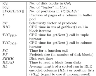
|Ci| No. of disk blocks inColi
||Ci|| No. of “tuples” inColi
||P OSLIST|| No. of positions inP OSLIST
F Fraction of pages of a column in buffer
pool
SF Selectivity factor of predicate
BIC CPU time in ms of getNext() call in
block iterator
T ICT U P CPU time for getNext() call in tuple
iterator
T ICCOL CPU time for getNext() call in column
iterator
F C Time for a function call
P F Prefetch size (in number of disk blocks)
SEEK Disk seek time
READ Time to read a block from disks
RL Average length of a sorted run in RLE
encoded columns (RLc) or position lists
(RLp) (equal to one if uncompressed)
Table 1: Notation used in analytical model
• AND operators that merge several filtered
posi-tion vectors or tuples with posiposi-tions together into a smaller list of positions.
• Tuple construction operators that combine
nar-row tuples of positions and values into wider columns with positions and multiple values. We use the notation in Table 1 to describe the costs of the different operators.
3.2 Data Sources
In this section, we consider the cost of accessing a col-umn on disk via a data source operator. We consider four cases:
Case 1: A column Ci of |Ci| blocks is read from
disk and a predicate with selectivitySF is applied to each tuple. The output is a column of positions. The pseudocode and cost analysis of this case is shown in Figure 1.
DS_Scan-Case1(Column C, Pred p) 1. for each block b in C 2. read b from disk
3. for each RLE tuple t in b 4. apply p to t
5. output positions from t
CP U = |Ci| ∗BIC+ (1) ||Ci|| ∗(T ICCOL+F C)/RL+ (3,4) SF∗ ||Ci|| ∗F C (5) IO=(|Ci| P F ∗SEEK+|Ci| ∗READ)∗(1−F) (2)
Figure 1: Psuedocode and cost formulas for data
sources, Case 1. Numbers in parentheses in cost for-mula indicate corresponding steps in the pseudocode. Case 2: A column Ci of |Ci| blocks is read from
disk and a predicate with selectivity SF is applied
to each tuple. The output is a column of (positions, value) pairs.
The cost of Case 2 is identical to Case 1 except for step (5) which becomes SF ∗ ||Ci|| ∗(T ICT U P + F C). The slightly higher cost reflects the cost of gluing positions and values together for the output.
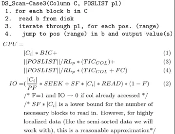
Case 3: A column Ci of |Ci| blocks is read from disk or memory and filtered with a list of positions,
P OSLIST. The output is a column of the values cor-responding to those positions. The pseudocode and cost analysis of this case is shown in Figure 2.
DS_Scan-Case3(Column C, POSLIST pl) 1. for each block b in C
2. read b from disk
3. iterate through pl, for each pos. (range) 4. jump to pos (range) in b and output value(s)
CP U = |Ci| ∗BIC+ (1) ||P OSLIST||/RLp∗(T ICCOL)+ (3) ||P OSLIST||/RLp∗(T ICCOL+F C) (4) IO=(|Ci| P F ∗SEEK+SF∗ |Ci| ∗READ)∗(1−F) (2)
/* F=1 and IO→0 if col already accessed */ /*SF∗ |Ci|is a lower bound for the number of
necessary blocks to read in. However, for highly localized data (like the semi-sorted data we will work with), this is a reasonable approximation*/
Figure 2: Psuedocode and cost formulas for data
sources, Case 3.
Case 4: A column Ci of |Ci| blocks is read from
disk and a set of tuples EMi of the form (pos, <
a1, . . . , an >) is input to the operator. The operator
jumps to the positionposin the column and a
predi-cate with selectivitySF is applied. Tuples that satisfy
the predicate are merged with EMi to create a tuple
of the form (pos, < a1, . . . , an, an+1 >) that contains
only the positions that were in EMi and that
satis-fied the predicate over Ci. The pseudocode and cost
analysis of this case is shown in Figure 3.
DS_Scan-Case4(Column C, Pred p, Table EM) 1. for each block b in C
2. read b from disk
3. iterate through tuples e in EM, extract pos 4. use pos to jump to correct tuple t in C
and apply predicate
5. if predicate succeeded, output <e, t>
CP U= |Ci| ∗BIC+ (1) ||EMi|| ∗T ICT U P+ (3) ||EMi|| ∗((F C+T ICT U P) +F C) (4) SF∗ ||EMi|| ∗(T ICT U P) (5) IO=(|Ci| P F ∗SEEK+|Ci| ∗READ)∗(1−F) (2)
Figure 3: Psuedocode and cost formulas for data
sources, Case 4.
3.3 Multicolumn AND
The AND operator can be thought of as taking ink po-sition lists,inpos1. . . inposk and producing a new list
of positions that represents the intersection of the two input lists,outpos. This model examines two possible representations for a list of positions: a list of ranges of positions(e.g., 1-100, 200-250) and bit-strings with one bit per position. The AND operator is only used in the LM case, since EM always uses Data scan Case 4 above to construct tuples as they are read from disk. If the positional input to AND are all ranges, then it will output position ranges. Otherwise it will output positions in bit-string format.
We consider three cases:
Case 1: Range inputs, Range output
In this case, each of the input position lists and the output position list are each encoded as ranges. The pseudocode and cost analysis for this case is shown in Figure 4. Since this operator is a streaming operator it incurs no I/O.
AND(POSLIST inpos 1 ... inpos k) 1. iterate through position lists 2. perform AND operations
3. produce output lists
LetM=max(||inposi||/RLpi, i∈1. . . k)
COST= X i=1...k (T ICCOL∗ ||inposi||/RLpi)+ (1) M∗(k−1)∗F C+ (2) M∗T ICCOL∗F C (3)
Figure 4: Psuedocode and cost formulas for AND,
Aase 1.
Case 2: Bit-list inputs, bit-list output In this case each of the input position lists and the output position lists are bit vectors. The input posi-tion lists are ”ANDed” 32 bits at a time. The cost formula for this case is identical to Case 1 except that every instance of||inposi||/RLpiin Figure 4 is replaced
with||inposi||/32 (32 is the processor word size). Case 3: Mix of Bit-list and range inputs, bit-list output
In this case the input position lists to the AND operator are a mix of range and bit lists. The output is a bit-list. Execution occurs in three steps. First the range lists are intersected to produce one range list. Second, the bit-lists are anded together to produce a single bit list. Finally, the single range and bit lists are combined to produce the output list.
3.4 Tuple Construction Operators
The final two operators we consider are tuple construc-tion operators. The first, the MERGE operator, takes
ksets of valuesV AL1. . . V ALk and produces a set of k-ary tuples. This operator is used to construct tuples
at the top of an LM plan. The pseudocode and cost of this operation is shown in Figure 5.
Merge(Col s1,..., Col sk)
1. iterate through all k cols of len. ||VAL_i|| 2. produce output tuples
COST=
// Access values as vector (don’t use iterator)
||V ALi|| ∗k∗F C+ (1)
// Produce tuples as array (don’t use iterator)
||V ALi|| ∗k∗F C) (2)
Figure 5: Psuedocode and cost formulas for Merge.
This analysis assumes that we have an iterator over each of the input streams, that all of the input streams are memory resident, and that only one iterator is needed to produce the output stream.
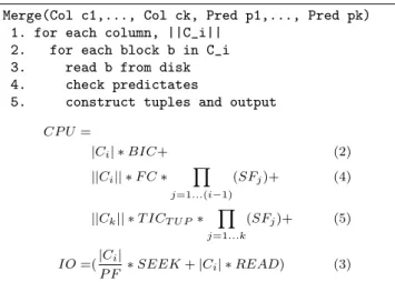
The second tuple construction operator is the SPC (Scan, Predicate, and Construct) operator which can sit at the bottom of EM plans. SPC takes a set of columnsV AL1. . . V ALk, reads them off disk,
option-ally takes a set of predicates to apply on the column values, and constructs tuples if all predicates pass. The pseudocode and cost of this operation is shown in Fig-ure 6.
Merge(Col c1,..., Col ck, Pred p1,..., Pred pk) 1. for each column, ||C_i||
2. for each block b in C_i 3. read b from disk 4. check predictates
5. construct tuples and output
CP U= |Ci| ∗BIC+ (2) ||Ci|| ∗F C∗ Y j=1...(i−1) (SFj)+ (4) ||Ck|| ∗T ICT U P ∗ Y j=1...k (SFj)+ (5) IO=(|Ci| P F ∗SEEK+|Ci| ∗READ) (3)
Figure 6: Psuedocode and cost formulas for SPC.
3.5 Example Query Plans
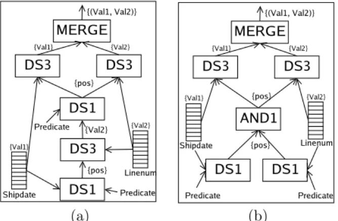
The use of these operators is illustrated in Figures 7 and 8 for the query:
SELECT shipdate, linenum
FROM lineitem
WHERE shipdate < CONST1
AND linenum < CONST2
where lineitem is a C-Store projection consisting
of the columns return f lag, shipdate, linenum, and
quantity. The primary and secondary sort keys for the lineitem projection are returnf lag and shipdate, respectively.
(a) (b)
Figure 7: Query plans for piplined (a) and EM-parallel (b) strategies
One EM query plan, shown in Figure 7(a),
uses a DS2 operator (Data Scan Case 2) operator to scan the shipnum column, producing a stream of (pos, shipdate) tuples that satisfy the predicate
shipdate < CON ST1. This stream is used as one in-put to a DS4 operator along with the linenum column
and the predicatelinenum < CON ST2 to produce a
stream of (shipnum, linenum) result tuples.
Another possible EM query plan, shown in Figure 7(b), contructs tuples at the very beginning of the plan - merging all needed columns at the leaf node as it ap-plies the predicates using a SPC operator. The key difference between these early materialization strate-gies is that while the latter strategy has to scan and process all blocks for all input columns, the former plan applies each predicate in turn, and will construct a tuple incrementally, adding one attribute per opera-tor. For non-selective predicates this is more work, but for selective predicates only subsets of blocks need to be processed (or in some cases the entire block can be skipped). We call the former strategy EM-pipelined
and the latter strategy EM-parallel. The choice of
which EM plan to use depends on the selectivity of the predicates (the former strategy likely is better if there are highly selective predicates).
Similarly to EM, there are both pipelined and par-allel late materialization strategies. LM-pipelined is shown in Figure 8(a) and LM-parallel is shown in Fig-ure 8(b). LM-parallel begins with two DS1 operators, one for the shipnum and linenum columns. Each DS1 operator scans its column, applying the appropriate predicate to produce a position list of those values that satisfy the predicate. The two position lists are streamed into an AND operator which intersects the two lists. The output position list is then streamed into two DS3 operators to obtain the correspond-ing values from the shipnum and linenum columns. As these values are obtained they are streamed into a merge operator to produce a stream of (shipnum, linenum) result tuples.
(a) (b)
Figure 8: Query plans for piplined (a) and LM-parallel (b) strategies
LM-pipelined works similarly to LM-parallel, ex-cept that it applies the DS1 operators one at a time, pipelining the positions of the shipdate values that passed the shipdate predicate to a DS3 operator for the linenum column which produces the column values at these input set of positions and sends these values to the linenum DS1 operator which only needs to ap-ply its predicate to this value subset (rather than at all linenum positions). As a result, the need for the AND operator is obviated.
3.6 LM Optimization: Multi-Columns
Note that in DS Case 3, used in LM strategies to pro-duce values from positions, the I/O cost is assumed to be zero if the column has already been accessed ear-lier in the plan, even if the column size is larger than available memory. This is made possible through a specialized data structure for representing intermedi-ate results, designed to facilitintermedi-ate query pipelining, that allows blocks of column data to remain in user mem-ory space after the first access so that it can be easily reaccessed again later on. We call this data structure amulti-column.
A multi-column contains a memory-resident, hor-izontal partition of some subset of attributes from a particular relation. It consists of:
A covering position range indicating the virtual
start position and end position of the horizontal parti-tion (for example, a posiparti-tion range could indicate that rows numbered 1000-2000 are covered in this multi-column).
An array ofmini-columns. A mini-column is the set corresponding values for a specified position range of a particular attribute (MonetDB [7] calls this a vec-tor, PAX [4] calls this amini-page). Using the previ-ous example, a mini-column for column X would con-tain 1001 values - the 1000th-2000th values in this
col-umn. Thedegree of a multi-column is the size of the
mini-column array which is the number of included attributes. Each mini-column is kept compressed the
same way as it was on disk.
A position descriptorindicating which positions in the position range remain valid. Positions are made invalid as predicates are applied on the multi-column. The position descriptor may take one of three forms:
• Ranged positions: All positions between a speci-fied start and end position are valid.
• Bit-mapped positions: A bit-vector of size equal to the multi-column covering position range is given, with a ’1’ at a corresponding position if that po-sition is valid. For example, for a popo-sition cov-erage of 11-20, a bit-vector of 0111010001 would indicate that positions 12, 13, 14, 16, and 20 are valid.
• Listed positionsA list of valid positions inside the covering position range is given. This is partic-ularly useful when few positions inside a
multi-column are valid. Multi-multi-columns may becollapsed
to contain only values at valid positions inside the mini-columns, in which case the position descrip-tor must be transformed tolisted positionsformat if positional information is still necessary for up-stream operators.
When a page from a column is read from disk (say, for example, by a DS1 operator), a mini-column is cre-ated (which is essentially just a pointer to the page in the buffer pool) and the position descriptor indicates that every value begins as being valid. The DS1 op-erator then iterates through the column, applying the predicate to each value, and produces a new list of po-sitions that are valid. The multi-column then replaces its position descriptor with the new position list (the mini-column remains untouched).
The AND operater then takes two multi-columns with overlapping covering position ranges, and creates a new multi-column where the covering position range and position descriptor is equal to the intersection of the position range and position descriptors of the input multi-columns, and the set of mini-columns is equal to the union of the input set of mini-columns. Thus, ANDing multi-columns is in essence the same oper-ation as the AND of positions shown in Section 3.3; the only difference is that on top of performing the in-tersection of the position lists, ANDing multi-columns must also copy pointers to mini-columns to the output multi-column, but this can be thought of as a zero-cost operation.
If the AND operator produces multi-columns rather than just positions as an input to a DS3 operator, then the operator does not need to reaccess the column, but rather can work directly on one multi-column block at a time - iterating through the appropriate mini-column to produce only those values whose positions are valid according to the position descriptor. Single multi-columns blocks are worked on in each operator
iteration, so that column-subsets can be pipelined up the query tree. With this optimization, DS3 I/O cost for a reaccessed column can be assumed to be zero.
...
0 1 1 0 0 1 1 1 0 0 1 1 0 0 1 Position descriptor Start 47 End 61 LINENUM values (encoded) RLE val = 5 start = 49 len = 15 RETFLAG values (encoded) Bit-vector 1 0 0 0 1 0 0 0 0 1 0 0 0 0 1 0 0 1 1 0 0 1 0 0 0 1 0 0 1 0 1 0 0 0 0 1 0 1 0 0 1 0 1 0 0 start = 47 values (65,78,82) SHIPDATE values (encoded) Uncomp. 8040 8041 8042 8043 8044 8044 8046 8047 8048 8048 8050 8051 8052 8053 8054Figure 9: An example MultiColumn block
con-taining values for the SHIPDATE, RETFLAG, and LINENUM columns. The block spans positions 47 to 61; within this range, positions 48, 49, 52, 53, 54, 57, 58, and 61 are active.
3.7 Predicted versus Actual Behavior
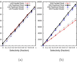
To gauge the accuracy of the analytical model we com-pared the predicated execution time for the selection query above with the actual execution time obtained using the C-Store prototype using a scale 10 version of the LineItem projection. The results obtained are pre-sented in Figures 10(a) and 10(b), which plot response time as a function of the selectivity of the predicate
shipdate < CON ST2 for the the late and early ma-terialization strategies respectively. The shipnum and linenum columns are both encoded using RLE encod-ing. The encoded sizes of the two columns are 1 block (3,800 tuples) and 5 blocks (26,726 tuples), respec-tively. Table 2 contains the constant values used by the analytical model which were obtained by running the small segments of code that only performed the variable in question (they were not reverse engineered to get the model to match the experiments). Both the model and the experiments incurred an additional cost at the end of the query to iterate through the output tuples (numOutT uples∗T ICT U P).
At this point, the important thing to observe is that the estimated performance from the EM and LM ana-lytical models are quite accurate at predicting the ac-tual performance of the C-Store prototype (at least for this query), providing a degree of reassurance regard-ing our understandregard-ing of how the two implementations actually work. A discussion on why the graphs look
BIC 0.020 microsecs T ICT U P 0.065 microsecs T ICCOL 0.014 microsecs F C 0.009 microsecs P F 1 block SEEK 2500 microsecs READ 1000 microsecs
Table 2: Constants used for Analytical Models the way they do will be included in Section 4. We also modelled the same query but did not compress the linenum column (linenum was 60,000,000 tuples occu-pying 916 64KB blocks) and modelled different queries (including allowing both the shipdate and the linenum predicates to vary). We consistently found the model to reasonably predict our experimental results.
0 1000 2000 3000 4000 5000 6000 7000 0 0.1 0.2 0.3 0.4 0.5 0.6 0.7 0.8 0.9 1 Runtime (ms) Selectivity (fraction) LM-Parallel Real LM-Pipelined Real LM-Pipelined Model LM-Parallel Model 0 2000 4000 6000 8000 10000 12000 14000 0 0.1 0.2 0.3 0.4 0.5 0.6 0.7 0.8 0.9 1 Selectivity (fraction) EM-Parallel Real EM-Pipelined Real EM-Pipelined Model EM-Parallel Model (a) (b)
Figure 10: Predicated and observed query
perfor-mance for late (a) and early (b) materialization strate-gies on selection queries
4
Experiments
To evaluate the trade-offs between the early materi-alization and late materimateri-alization strategies, we ran two queries under a variety of configurations. These queries were run over data generated from the TPC-H dataset, a benchmark that models data typically found in decision support and data warehousing ap-plications. Specifically, we generated an instance of the TPC-H data at scale 10, which yields a total database size of approximately 10GB with the biggest
table (lineitem) containing 60,000,000 tuples. We
then created a C-Store projection (which is a sub-set of columns from a table all sorted in the same order) of the SHIPDATE, LINENUM, QUANTITY, and RETURNFLAG columns; the projection was pri-marily sorted on RETURNFLAG, secondarily sorted on SHIPDATE, and tertiarily sorted on LINENUM. The RETURNFLAG and SHIPDATE columns were compressed using run-length encoding, the LINENUM
column was stored redundantly using uncompressed, RLE, and bit-vector encodings, and the QUANTITY column was left uncompressed..
We ran the two queries on these data. First, we ran a simple selection query:
SELECT SHIPDATE, LINENUM FROM LINEITEM
WHERE SHIPDATE < X AND LINENUM < Y
where X and Y are both constants. Second, we ran
an aggregation version of this query: SELECT SHIPDATE, SUM(LINENUM) FROM LINEITEM
WHERE SHIPDATE < X AND LINENUM < Y GROUP BY SHIPDATE
again withX andY as constants. While these queries
are simpler than those that one would expect to see in a production environment, they are able to illustrate from a more fundamental level the essential differences in performance between the three strategies. We look at joins in Section 4.3.
To explore the performance of the materialization strategies as a function of the selectivity of the query,
we varied X across the entire shipdate domain and
kept Y constant at 7 (96% selectivity). In other ex-periments (not presented in this paper) we varied Y and kept X constant and observed similar results (un-less otherwise stated).
Additionally, at each point in this sample space, we varied the encoding of the LINENUM column among uncompressed, RLE, and bit-vector encodings (SHIP-DATE was always RLE encoded). We experimented with the four different query plans described in Section
3.5: EM-pipelined, EM-parallel, LM-pipelined, and
LM-parallel. Both LM strategies were implemented
using the multi-column optimization.
Experiments were run on a Dell Optiplex GX620 DT with a 3.8 GHz Intel Pentium 4 processor 670 with HyperThreading, 2MB of cache, and a 800 Mhz FSB. The system had 4GB of main memory installed, of which 3.5GB were available to the operating sys-tem. The hard drive used was a 250GB Western Dig-ital WD2500JS-75N.
4.1 Experiment 1: Simple Selection Query
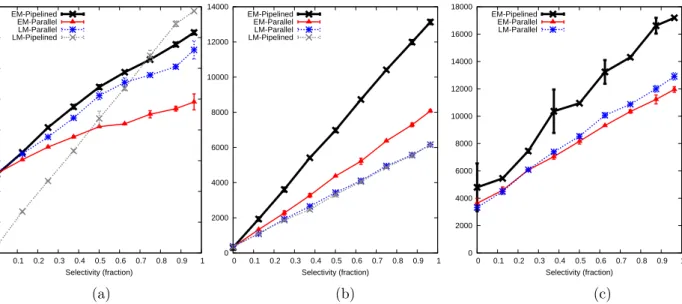
For this set of experiments, we consider the simple se-lection query presented both in Section 3.5 and in the introduction to this section above. Figure 11 (a), (b), and (c) shows the total end-to-end query time for the four materialization strategies when the LINENUM column stored uncompressed, RLE encoded, and bit-vector encoded respectively.
For the uncompressed LINENUM experiment (Fig-ure 11 (a)), LM-pipelined is the clear winner at low
selectivities. This is because the pipelined algorithm saves both I/O and CPU costs of reading in and apply-ing the predicate to the large (250 MB) uncompressed LINENUM column since the first predicate is so se-lective and the matching tuples are so localized (since the SHIPDATE column is secondarily sorted) that en-tire LINENUM blocks can be skipped from being read in and processed. However at high selectivities LM-pipelined performs particularly poorly since the CPU cost of jumping to each matching position is more ex-pensive than iterating through the block one position at a time if most positions will have to be jumped to. This additional CPU cost eventually dominates query time. At high selectivities, immediately making complete tuples at the bottom of the query plan (EM-parallel) is the best thing to do. EM-parallel consis-tently outperforms LM-parallel since the LINENUM predicate selectivity is so high (96%). In other exper-iments (not shown), we varied the LINENUM predi-cate across the LINENUM domain and observed that if both the LINENUM and the SHIPDATE predicate have medium selectivities, LM-parallel can beat EM-parallel (this is due to the LM advantage of waiting until the end of the query to construct tuples and thus it can avoid creating tuples that will ultimately not be output).
For the RLE-compressed LINENUM experiment (Figure 11 (b)), the I/O cost for all materialization strategies is negligible (the RLE encoded LINENUM column occupies only three 64k blocks on disk). At low query selectivities, the CPU cost is also minimal for all strategies and they all perform on the order of tens to hundreds of milliseconds. However, as the query se-lectivity increases, we observe the difference in costs of the strategies. Both EM strategies under-perform the LM strategies since tuples are constructed at the beginning of the query plan and tuple construction re-quires the RLE-compressed data to be decompressed (Section 2.1.2) precluding the performance advantages of operating directly on compressed data discussed in [3]. In fact the CPU cost of operating directly on com-pressed data is so small that the almost the entire query time for the LM strategies is the construction of the tuples and subsequent iteration over the results; hence both LM strategies perform similarly.
For the bit-vector compressed LINENUM experi-ment (Figure 11 (c)), we show the results for only three strategies since performing position filtering di-rectly on bit-vector data (the DS3 operator) is not supported (since it is impossible to know in advance in which bit-string any particular position is located). Further, the advantage of reducing the number of val-ues that the predicate has to be applied to for the LM-pipelined strategy is irrelevant for the bit-vector compression technique (since the predicate has already been applied a-priori as each bit-vector is a list of posi-tions that match a particular value equality predicate
0 2000 4000 6000 8000 10000 12000 14000 16000 0 0.1 0.2 0.3 0.4 0.5 0.6 0.7 0.8 0.9 1 Runtime (ms) Selectivity (fraction) EM-Pipelined EM-Parallel LM-Parallel LM-Pipelined 0 2000 4000 6000 8000 10000 12000 14000 0 0.1 0.2 0.3 0.4 0.5 0.6 0.7 0.8 0.9 1 Selectivity (fraction) EM-Pipelined EM-Parallel LM-Parallel LM-Pipelined 0 2000 4000 6000 8000 10000 12000 14000 16000 18000 0 0.1 0.2 0.3 0.4 0.5 0.6 0.7 0.8 0.9 1 Selectivity (fraction) EM-Pipelined EM-Parallel LM-Parallel (a) (b) (c)
Figure 11: Run-times for four materialization strategies on selection queries with uncompressed (a), RLE com-pressed (b), and Bit-vector comcom-pressed (c) LINENUM column
- to apply a range predicate, the executor simply needs to OR together the relevant bit-vectors). Thus, only one LM algorithm is presented (LM-parallel).
Since there are only 7 unique LINENUM values, the bit-vector compressed column is a little less than 25% of the size on disk of the uncompressed column. Thus, the dominant cost of the query is the CPU cost of decompressing the bit-vector data which has to be done for both the LM and EM strategies. Hence, EM-parallel and LM-EM-parallel perform similarly.
4.2 Experiment 2: Aggregation Queries
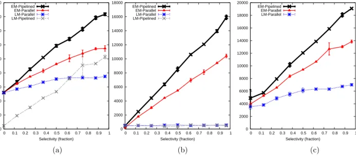
For this set of experiments, we consider adding an ag-gregation operator on top of the selection query plan (the full query is presented in the introduction to this section above). Figure 12 (a), (b), and (c) shows the total end-to-end query time for the four materializa-tion strategies when the LINENUM column stored un-compressed, RLE encoded, and bit-vector encoded re-spectively.
In each of these three graphs, the EM strategies per-form similarly to their counterpart in Figure 11. This is because the CPU cost of iterating through the query results in Figure 11 is done by the aggregator (and the cost to iterate through the aggregated results and to perform the aggregation itself is minimal). However, the LM strategies all perform significantly better. In the uncompressed case (Figure 12(a)) this is because waiting to construct tuples is a big win since the aggre-gator significantly reduces the number of tuples that need to be constructed. For the compressed cases (Fig-ure 12(a) and (b)) the aggregator iterator cost is also reduced since it can optimize its performance by oper-ating directly on compressed data [3] so keeping data
compressed as long as possible is also a win.
4.3 Joins
We now look at the effect of materialization strategy on join performance. If an early materialization strat-egy is used relative to a join, tuples have already been constructed before reaching the join operator, so the join functions as it would in a standard row-store sys-tem, with tuples being output. However, an alterna-tive algorithm can be used if using a late materializa-tion strategy. In this case, only columns that compose the join predicate are input to the join. The output of the join is set of pairs of positions in the two input relations for which the predicate succeeded. For ex-ample, the figure below shows the results of a join of a column of size 5 with a column of size 3.
42 36 42 44 38
o
n
38 42 46 = 1 2 3 2 5 1For most join algorithms, the output positions for the left input relation will be sorted while the output positions of the right input relation will not. This is because the positions in the left column are usually iterated through in order, while the right relation is probed for join predicate matches. This asymmetric nature of join positional output implies that restrict-ing other columns from the left input relation usrestrict-ing the join output positions will be relatively fast (the stan-dard merge join of positions can be used to extract col-umn values); however, restricting other colcol-umns from the right input relation using the join output positions can be significantly more expensive (out of order
0 2000 4000 6000 8000 10000 12000 14000 16000 18000 0 0.1 0.2 0.3 0.4 0.5 0.6 0.7 0.8 0.9 1 Runtime (ms) Selectivity (fraction) EM-Pipelined EM-Parallel LM-Parallel LM-Pipelined 0 2000 4000 6000 8000 10000 12000 14000 16000 18000 0 0.1 0.2 0.3 0.4 0.5 0.6 0.7 0.8 0.9 1 Selectivity (fraction) EM-Pipelined EM-Parallel LM-Parallel LM-Pipelined 0 2000 4000 6000 8000 10000 12000 14000 16000 18000 20000 0 0.1 0.2 0.3 0.4 0.5 0.6 0.7 0.8 0.9 1 Selectivity (fraction) EM-Pipelined EM-Parallel LM-Parallel (a) (b) (c)
Figure 12: Run-times for four materialization strategies on aggregation queries with uncompressed (a), RLE compressed (b), and Bit-vector compressed (c) LINENUM column
tions implies that a merge-join on position cannot be used to fetch column values).
Of course, a hybrid approach can be used where the right relation can send tuples to the join operator, while the left relation can send the single join pred-icate column. The join result is then a set of tuples from the right relation and an ordered set of positions from the left relation which can then be used to fetch values from relevant columns in the left relation to complete the tuple stitching process and create a sin-gle join result tuple. This allows for the advantage of only having to materialize values in the left relation for tuples that passed the join predicate without paying the penalty of an extra non-merge positional join with the right relation.
Multi-columns give joins another option as an al-ternative right (inner) table representation instead of forcing input tuples to be completely constructed or just sending the join predicate column. All relevant columns (columns that will be materialized after the join in addition to columns in the join predicate) are input to the join operator and as inner table values match the join predicate, the position of this value is extracted and used to get the appropriate value in all of the other relevant columns and the tuple constructed on the fly. This hybrid technique is useful if the join selectivity is low, and few tuples need be constructed. To further examine the differences between these three materialization approaches for the inner table in a join operator (send just the unmaterialized join predicate column, send the unmaterialized relevant columns in a multi-column, or send materialized tu-ples), we ran a standard star schema join query on our TPC-H data between the orders table and customers
table on customer key (customer key is a foreign key in the orders table and the primary key for the customers table), varying the selectivity of an input predicate on the orders table:
SELECT Orders.shipdate Customer.nationcode
FROM Orders, Customer
WHERE Orders.custkey=Customer.custkey AND Orders.custkey < X 0 20000 40000 60000 80000 100000 120000 140000 160000 0 0.1 0.2 0.3 0.4 0.5 0.6 0.7 0.8 0.9 1 Runtime (ms) Selectivity (fraction)
Right Table Materialized Right Table Multi-Column Right Table Single Column
Figure 13: Run-times for three different materializa-tion strategies for the inner table of a join query
Where X is varied so that a desired predicate se-lectivity can be acquired. For TPC-H scale 10 data, the orders table contains 15,000,000 tuples and the customer table 1,500,000 tuples and since this is a for-eign key-primary key join, the join result will also have at most 15,000,000 tuples (the actual number is deter-mined by the Orders predicate selectivity). The results of this experiment can be found in Figure 13.
Sending early materialized tuples and multi-column unmaterialized column data to the right-side input of the join operator results in similar performance num-bers since the the multi-column advantage of only ma-terializing relevant tuples is not helpful for a foreign key-primary key join of this type where there are ex-actly as many join results as there are join inputs. Sending just the join predicate column (“pure” late materialization) performs poorly due to the extra join of right-side positions. If the entire set of positions were not able to be kept in memory, late materializa-tion would have performed even worse.
We do not present results for varying the material-ization strategy of the left-side input table to the join operator since the issues at play are identical to the is-sues discovered in the previous experiments: if the join is highly selective or if the join results will be aggre-gated, a late materialization strategy should be used. Otherwise, EM-parallel should be used.
5
Related Work
The multi-column idea of combining chunks of columns covering the same position range together into one data structure is similar to the PAX [4] idea of taking a row-store page and splitting it into multiplemini-pages where each tuple attribute is stored contiguously. PAX does this to improve cache performance by maximiz-ing inter-record spatial locality within a page. Multi-columns build on the PAX idea in the following ways: First, multi-columns are an in-memory data structure only and are created on the fly from different columns stored separately on disk (where pages for the different columns on disk do not necessarily match-up position-wise). Second, positions are first class citizens in multi-columns and may be accessed and processed separately from attribute values. Finally, mini-columns are kept compressed inside multi-columns in their native com-pression format throughout the query plan, encapsu-lated inside a specialized data structures that facilitate direct operation on compressed data.
To the best of our knowledge, this paper contains the only study of multiple tuple creation strategies in a column-oriented system. C-Store [16] used LM-parallel only (until we extended it with additional strategies). Published descriptions of Sybase IQ [11] seem to indicate that they also perform LM-parallel. Ongoing work by Halverson et. al. [8] and
Harizopou-los et. al. [9] that further explores the trade-offs
between row- and column-stores use early material-ization approaches for the column-store they imple-mented (the former uses EM-parallel, the latter uses
EM-pipelined). MonetDB/X100 [7] uses late
mate-rialization implemented using a similar multi-column approach; however their version of position descriptors (they call themselection vectors) are kept separately from column values and data is decompressed in the cache, precluding the potential performance benefits
of operating directly on compressed data both on po-sition descriptors and on column values.
Finally, we used the analytical model presented in [8] as a starting point for the analytical model we pre-sented in Section 3. However, we extended their model since they look only at scanning costs of the leaf query plan operators whereas we model the costs for the en-tire query since the query plans for different material-ization strategies have different costs.
6
Conclusion
The optimal point at which to perform tuple con-struction in a column-oriented database is not obvious. This paper provides a systematic evaluation of a vari-ety of strategies for when tuple construction should oc-cur. We showed that late materialization has many ad-vantages, but potentially incurs additional costs due to re-processing disk blocks, and hence early materializa-tion is sometimes preferable. A good heuristic to use is that if output data is aggregated, or if the query has low selectivity (highly selective predicates), or if input data is compressed using a light-weight compression technique, a late materialization strategy should be used. Otherwise, for high selectivity, non-aggregated, non-compressed data, early materialization should be used. Further, the right input table to a join should be materialized before (or during if a multi-column is input) the join operation. Using an analytical model to predict query performance can facilitate material-ization strategy decision-making.
References
[1] http://www.addamark.com/products/sls.htm.
[2] C-store code release under bsd license. http://
db.csail.mit.edu/projects/cstore/, 2005.
[3] D. J. Abadi, S. Madden, and M. Ferreira. In-tegrating compression and execution in
column-oriented database systems. InSIGMOD, 2006.
[4] A. Ailamaki, D. J. DeWitt, M. D. Hill, and M. Sk-ounakis. Weaving relations for cache performance.
InVLDB ’01, pages 169–180, San Francisco, CA,
USA, 2001.
[5] P. Boncz. Monet: A next-generation dbms ker-nel for query-intensive applications. Phd thesis, Universiteit van Amsterdam, 2002.
[6] P. A. Boncz and M. L. Kersten. MIL primitives
for querying a fragmented world. VLDB Journal:
Very Large Data Bases, 8(2):101–119, 1999. [7] P. A. Boncz, M. Zukowski, and N. Nes.
Mon-etdb/x100: Hyper-pipelining query execution. In
[8] A. Halverson, J. Beckmann, and J. Naughton. A principled comparison of storage optimizations for row-store and column-store systems for
read-mostly query workloads. in submission. http:
//www.cs.wisc.edu/∼alanh/tr.pdf.
[9] S. Harizopoulos, V. Liang, D. Abadi, and S.
Mad-den. Performance tradeoffs in read-optimized
databases. InVLDB, page To appear, 2006.
[10] Kx Sytems, Inc. Faster database platforms
for the real-time enterprise: How to get the
speed you need to break through business
intelligence bottlenecks in financial
institu-tions. http://library.theserverside.com/
data/document.do?res id=1072792428 967,
2003.
[11] R. MacNicol and B. French. Sybase IQ multiplex
- designed for analytics. InVLDB, pages 1227–
1230, 2004.
[12] P. E. O’Neil and D. Quass. Improved query
per-formance with variant indexes. In Proceedings
ACM SIGMOD ’97 Tucson, Arizona, USA, pages
38–49, 1997.
[13] R. Ramamurthy, D. Dewitt, and Q. Su. A case for fractured mirrors. InVLDB, 2002.
[14] S. Khoshafian, et al. A query processing
strat-egy for the decomposed storage model. InICDE,
1987.
[15] P. Selinger, M. Astrahan, D. Chamberlin, R. Lo-rie, and T. Price. Access path selection in a
rela-tional database management system. In
Proceed-ings of the ACM SIGMOD Conference on
Man-agement of Data, pages 23–34, Boston, MA, 1979.
[16] M. Stonebraker, D. J. Abadi, A. Batkin, X. Chen, M. Cherniack, M. Ferreira, E. Lau, A. Lin, S. Madden, E. J. O’Neil, P. E. O’Neil, A. Rasin, N. Tran, and S. B. Zdonik. C-store: A