This item was submitted to Loughborough’s Institutional Repository
(
https://dspace.lboro.ac.uk/
) by the author and is made available under the
following Creative Commons Licence conditions.
For the full text of this licence, please go to:
Reliability Model Generation
by
Kathryn Sarah Stockwell
Doctoral Thesis
Submitted in partial fulfilment of the requirements for the award of
Doctor of Philosophy
of
Loughborough University
September 2013
c
There are many methods for modelling the reliability of systems based on component failure data. This task becomes more complex as systems increase in size, or undertake missions that comprise multiple discrete modes of operation, or phases. Existing techniques require certain levels of expertise in the model generation and calculation processes, meaning that risk and reliability assessments of systems can often be expensive and time-consuming. This is exacerbated as system complexity increases.
This thesis presents a novel method which generates reliability models for
phased-mission systems, based on Petri nets, from simple input files. The process has been
automated with a piece of software designed for engineers with little or no experience in the field of risk and reliability. The software can generate models for both repairable and non-repairable systems, allowing redundant components and maintenance cycles to be included in the model.
Further, the software includes a simulator for the generated models. This allows a user with simple input files to perform automatic model generation and simulation with a single piece of software, yielding detailed failure data on components, phases, missions and the overall system. A system can also be simulated across multiple consecutive missions. To assess performance, the software is compared with an analytical approach and found to match within ±5% in both the repairable and non-repairable cases.
The software documented in this thesis could serve as an aid to engineers designing new systems to validate the reliability of the system. This would not require specialist consultants or additional software, ensuring that the analysis provides results in a timely and cost-effective manner.
Keywords: Phased-Mission Systems, Automated, Model Generation, Simulation, Petri
I would like to thank my supervisor, Sarah Dunnett, for her support throughout my Ph.D. I would also like to thank Chris, Liz and Tom, particularly for their friendship and office shenanigans.
I would also like to thank Lockheed Martin who have given me time to complete this Ph.D. and those particularly at Lockheed Martin who took the time to ensure I could achieve this goal.
I would lastly like to thank both the Stockwell and Offer families for their love, support and unending encouragement throughout the last 4 years. My parents who have always been there for me and Tom, for everything.
List of Figures xiii
List of Tables xix
Principal Notation xxi
List of Acronyms xxiii
1 Introduction 1
1.1 Background . . . 1
1.2 Research Objectives . . . 2
1.3 Basic Definitions . . . 3
1.3.1 Hazard Rate . . . 3
1.3.2 Reliability and Unreliability . . . 3
1.3.3 Availability and Unavailability . . . 4
1.3.4 Maintenance Policies . . . 4
1.3.5 Cut Sets and Minimal Cut Sets . . . 6
1.3.6 Implicants and Prime Implicants . . . 6
1.4 Reliability Techniques . . . 6 1.4.1 Combinatorial . . . 6 1.4.2 State-Space . . . 19 1.4.3 Simulation . . . 24 1.5 Summary . . . 38 2 Phased-Mission Systems 39 2.1 Introduction . . . 39
2.1.1 Types of phased-mission systems . . . 40
2.1.2 Analytical Modelling Techniques . . . 41
2.2 Non-Repairable Systems . . . 41
2.2.1 Phase Fault Trees . . . 41
2.2.2 Phase Modular Approach . . . 54
2.2.3 Binary Decision Diagrams for Phased-Mission Systems . . . 57
2.3 Repairable Systems . . . 62
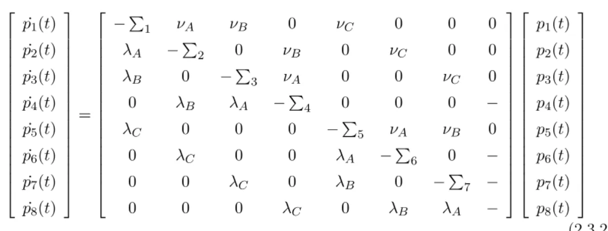
2.3.1 Markov applications in Phased-Mission Systems . . . 62
2.3.2 System and Phase Petri Nets . . . 69
3 Automated Techniques 73
3.1 Introduction . . . 73
3.2 Methods for Automation of Reliability Models . . . 73
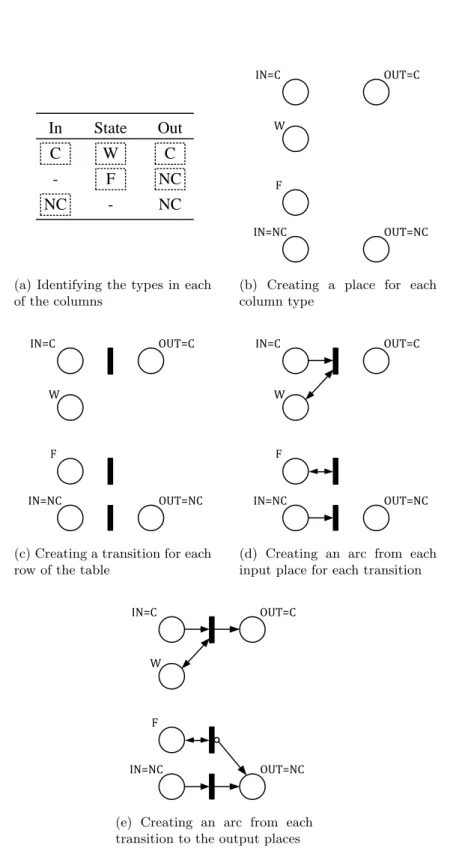
3.2.1 Decision Table Methods . . . 73
3.2.2 Digraph Method . . . 77
3.2.3 Modified Decision Table method . . . 77
3.2.4 Cause-Consequence Diagrams . . . 79
3.2.5 Mini fault trees . . . 79
3.2.6 Faultfinder . . . 79
3.3 Summary . . . 85
4 Modelling of Non-Repairable Systems 87 4.1 Introduction . . . 87 4.2 Model Inputs . . . 88 4.2.1 Component Description . . . 88 4.2.2 System Description . . . 91 4.2.3 Circuit Description . . . 92 4.2.4 Phase Description . . . 92 4.2.5 Initial Conditions . . . 92
4.3 Petri Net Models . . . 93
4.3.1 Component Petri Nets . . . 93
4.3.2 Circuit Petri Nets . . . 102
4.3.3 System Petri Nets . . . 104
4.3.4 Phase Petri Nets . . . 109
4.4 Algorithm . . . 115
4.5 Summary . . . 120
5 Application of the Procedure to Pressure Tank System 123 5.1 Introduction . . . 123
5.1.1 The Pressure Tank System . . . 124
5.2 System and Mission Description . . . 125
5.2.1 Components . . . 125
5.2.2 System Structure . . . 130
5.2.3 Circuits . . . 130
5.2.4 Mission Profile . . . 131
5.3 Pressure Tank System Model Construction . . . 131
5.3.1 Component and System Petri Nets . . . 132
5.3.2 Circuit Petri Nets . . . 132
5.3.4 The Completed Model . . . 142
5.4 Summary . . . 142
6 Automated Reliability Modelling 147 6.1 Introduction . . . 147
6.1.1 Object-Oriented Programming in C++ . . . 148
6.1.2 Key Definitions . . . 148
6.2 Software Files . . . 149
6.2.1 Component Description Files . . . 150
6.2.2 System Topology Description . . . 152
6.2.3 Mission Description . . . 153
6.2.4 Simulation File . . . 155
6.2.5 Setup File . . . 157
6.3 Software Structure . . . 158
6.3.1 Storage of System and Mission Description . . . 158
6.3.2 Building the Petri Net Model . . . 171
6.3.3 Simulating the Petri Net Model . . . 178
6.4 Testing and Validation . . . 187
6.4.1 Validation using Phase Fault Trees . . . 188
6.5 Summary . . . 196
7 Modelling of Repairable Systems 199 7.1 Introduction . . . 200 7.2 Preventative Maintenance . . . 201 7.2.1 File Input . . . 201 7.2.2 System Storage . . . 202 7.2.3 Construction Procedure . . . 203 7.3 Corrective Maintenance . . . 206 7.3.1 File Input . . . 207 7.3.2 System Storage . . . 207 7.3.3 Construction Procedure . . . 208 7.4 Standby Systems . . . 212 7.4.1 File Input . . . 212 7.4.2 System Storage . . . 215 7.4.3 Construction Procedure . . . 217 7.4.4 Cold Standby . . . 218 7.4.5 Warm Standby . . . 219 7.4.6 Hot Standby . . . 219 7.5 Voting Systems . . . 221
7.5.1 File Input . . . 221 7.5.2 System Storage . . . 222 7.5.3 Construction Procedure . . . 222 7.6 Mission Abort . . . 225 7.6.1 File Input . . . 225 7.6.2 System Storage . . . 225 7.6.3 Construction Procedure . . . 225
7.7 Simulating a Repairable System . . . 229
7.7.1 Simulation Algorithm . . . 229
7.7.2 Simulation of the model . . . 230
7.7.3 Simulating Transitions . . . 230
7.8 Repairable Bulb System . . . 230
7.8.1 Introduction . . . 230
7.8.2 System Description . . . 231
7.8.3 Mission Description . . . 234
7.8.4 Maintenance Plan . . . 234
7.8.5 Petri Net Models . . . 234
7.8.6 Validation . . . 237
7.9 Summary . . . 242
8 Conclusion and Further Work 243 8.1 Conclusion . . . 243
8.2 Further Work . . . 246
8.2.1 Optimisation Study . . . 246
8.2.2 Minimal Cut Sets . . . 246
8.2.3 Automatic Generation of the System Structure File . . . 247
8.2.4 Multiple Interacting Systems . . . 247
References 249 A User Interaction 255 A.1 Menu Interaction . . . 255
B Pressure Tank System 259 B.1 Input Files . . . 259
B.1.1 Project File . . . 259
B.1.2 Component Files . . . 260
B.1.3 System Structure File . . . 267
B.1.5 Simulation File . . . 271 B.1.6 Setup File . . . 273 B.2 Analytical Results . . . 273 B.2.1 Single Mission . . . 273 B.3 Simulation Results . . . 273 B.3.1 Single Mission . . . 273 B.3.2 Multiple Missions . . . 273 C Bulb System 279 C.1 Input Files . . . 279 C.1.1 Project File . . . 279 C.1.2 Component Files . . . 280
C.1.3 System Structure File . . . 282
C.1.4 Phase Transition Table File . . . 283
C.1.5 Simulation File . . . 284
1.1 The bath-tub curve . . . 3
1.2 Example fault tree . . . 10
1.3 Example reliability block diagram . . . 12
1.4 Reliability block diagram including series, parallel and voting systems . . . 15
1.5 Reliability block diagram analysis steps . . . 15
1.6 Example binary decision diagram . . . 16
1.7 Binary decision diagram illustrating ite(X1, f1, f2). . . 17
1.8 Simple fault tree structure for conversion to a binary decision diagram . . . 18
1.9 Markov model depicting a working, failed state system . . . 20
1.10 Two-component system . . . 25
1.11 Representation of direct sampling . . . 26
1.12 Working and failed state system . . . 29
1.13 Petri net with multiple transitions and multiple tokens in one place . . . 30
1.14 Petri net . . . 31
1.15 Petri net transition process . . . 32
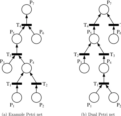
1.16 Petri net example and dual of the Petri net . . . 34
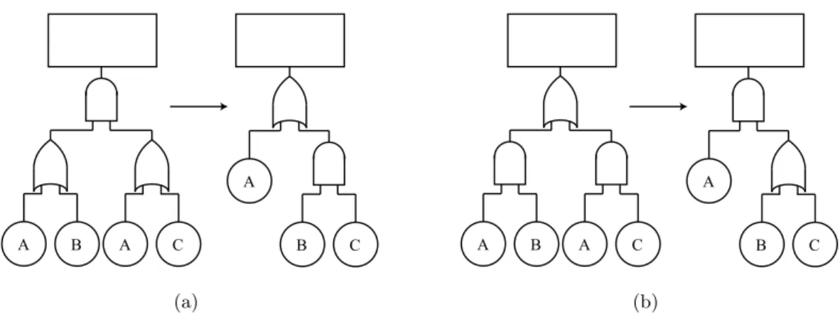
1.17 Petri nets illustrating absorption . . . 36
1.18 Petri net and the equivalent reachability graph . . . 38
2.1 Phased mission of an aircraft flight . . . 40
2.2 Process for a two phase mission to find the exact solution . . . 43
2.3 Generalised phase fault tree (La Band 2005) . . . 47
2.4 Three phased-mission system . . . 47
2.5 Phase fault tree construction of phase 2 . . . 48
2.6 Phase fault tree construction of phase 3 . . . 49
2.7 Extraction method for fault trees . . . 49
2.8 Modularised fault tree . . . 55
2.9 System configuration for a three phase mission . . . 62
3.1 Operator-driven valve . . . 76
3.2 FAULTFINDER Structure (Hunt et al. 1993) . . . 80
4.1 Power Supply component . . . 88
4.2 Switch component . . . 89
4.4 Example of a topology diagram . . . 91
4.5 Procedure steps for the construction of a Petri net representing a power supply 96 4.6 Procedure steps for the construction of a Petri net representing a toggle switch using the Operational Mode Transition (OMT) . . . 97
4.7 Procedure steps for the construction of a Petri net representing a toggle switch using the Decision Table (DT) . . . 99
4.8 Example of using failure rates in Petri net models . . . 101
4.9 Example of a component with multiple failure states and one operating mode101 4.10 Example of a system with multiple circuits . . . 103
4.11 Procedure steps for the construction of a Petri net representing circuit 1 . . 105
4.12 Petri net for current and no current in circuit 2 . . . 106
4.13 Petri net for the monitoring of the state of circuit 2 and the connection to the System Petri Net (SPN) . . . 106
4.14 Procedure steps for the construction of the system Petri net . . . 108
4.15 System diagram and topology for a heater and fan system . . . 113
4.16 Steps 1-5 of the construction procedure applied to the heater, fan system . . 116
4.17 Steps 6-8 of the construction procedure applied to the heater, fan system . . 117
4.18 Steps 9-10 of the construction procedure applied to the heater, fan system . 118 4.19 Flow chart of the algorithm . . . 121
5.1 Pressure Tank System . . . 124
5.2 Schematic of Pressure Tank System . . . 130
5.3 Component Petri Net (CPN) construction and integration of the component tables for the component push-switch (S1) . . . 133
5.4 Component Petri net of the failure rate for components S1,CR,CT and V . 134 5.5 Pressure Gauge ,P G, transitions between the working state and the different failure states . . . 134
5.6 Petri nets for components with multiple modes of operation . . . 135
5.7 Petri nets for components within circuits . . . 136
5.8 Component Petri nets for non-circuit components . . . 137
5.9 Part one of the system PN . . . 138
5.10 Part two of the system PN . . . 139
5.11 Part three of the system PN . . . 140
5.12 Part four of the system PN . . . 141
5.13 Circuit Petri Nets for Circuits 1 to 4 of the Pressure Tank System . . . 143
5.14 Circuit Petri Net for Circuit 5 of the Pressure Tank System . . . 144
5.15 Circuit Petri net linkage Petri nets . . . 145
6.1 Decision table file input format for single mode components . . . 151
6.2 Examples of the file format required for multiple mode components . . . 152
6.3 Example topology file format . . . 154
6.4 Example mission file format . . . 155
6.5 Example simulation file format . . . 156
6.6 Class view oftopSystem,fileHandler and compLib. . . 159
6.7 Class representation of the component class and its sub-classes . . . 160
6.8 First section of the algorithm for parsing and storing information within a .dtor .omtfile . . . 162
6.9 Second section of the algorithm for parsing and storing information within a.dt or.omt file . . . 163
6.10 First section of the algorithm for parsing and storing information within a .ssfile . . . 164
6.11 Second section of the algorithm for parsing and storing information within a.ss file . . . 165
6.12 Third section of the algorithm for parsing and storing information within a .ssfile . . . 166
6.13 First section of the algorithm for parsing and storing information within a .pttfile . . . 168
6.14 Second section of the algorithm for parsing and storing information within a.pttfile . . . 169
6.15 Third section of the algorithm for parsing and storing information within a .pttfile . . . 170
6.16 Process for the generation of the circuit lists . . . 172
6.17 Circuit detection method used for the circuit system in the pressure tank system . . . 173
6.18 Flow chart of the process of the simulation of a transition . . . 184
6.19 Flow chart of the process of the simulation of the model, part 1 . . . 185
6.20 Flow chart section of the process of the simulation of the model, part 2 . . . 186
6.21 Pressure tank system phase 1 fault tree . . . 189
6.22 Pressure tank system phase 2 fault tree . . . 189
6.23 Pressure tank system phase 3 fault tree . . . 190
6.24 Pressure tank system phase 4 fault tree . . . 190
6.25 Phase 2 simulation convergence results . . . 192
6.26 Phase 3 simulation convergence results . . . 193
6.27 Phase 4 simulation convergence results . . . 193
6.29 Section of the mission unreliability graph for a non-repairable pressure tank
system . . . 195
6.30 Individual phase unavailability over time . . . 196
6.31 Mission unavailability over time . . . 197
7.1 Petri net showing the transition between working, failed and under repair states of a component . . . 200
7.2 General preventative Petri net . . . 201
7.3 File Input expressions within the simulation file . . . 202
7.4 planDetails class view . . . 202
7.5 preventative class view . . . 202
7.6 maintenance class view . . . 203
7.7 Flow chart showing the steps to taking the file input and storing the preventative maintenance information . . . 204
7.8 Flow chart showing the steps to taking the file input and storing the preventative maintenance information . . . 207
7.9 corrective class view . . . 208
7.10 Flow chart for the process of taking in the file and interpreting the corrective maintenance plan . . . 209
7.11 Petri net for a single mode component under a corrective maintenance plan 212 7.12 Petri net for multiple components maintained by a single maintenance engineer213 7.13 Petri net for a system-wide corrective maintenance plan with two mainte-nance engineers . . . 214
7.14 Declarations used within the STANDBY header within the simulation file . 214 7.15 The standby class . . . 215
7.16 Flow chart for the storing of the standby components . . . 216
7.17 Example of power supplies in cold standby . . . 219
7.18 Example of work to fail to repair relationship for a single mode component in warm standby . . . 220
7.19 Example of power supplies in warm standby . . . 220
7.20 Example of power supplies in hot standby . . . 221
7.21 Example of aVOTING declaration . . . 222
7.22 The voting class . . . 222
7.23 Flow chart for the storing of the voting information . . . 223
7.24 An example of a 2-out-of-3 voting system Petri net . . . 224
7.25 File format for the ABORT header within the simulation file . . . 225
7.27 The first part of the software algorithm to populate the system with abort
conditions . . . 227
7.28 The second part of the software algorithm to populate the system with abort conditions . . . 228
7.29 Example representation of the abort process within a Phase Petri Net (PPN)228 7.30 Schematic of the bulb system . . . 231
7.31 System topology diagram for the bulb system . . . 232
7.32 CPNs for the components of the bulb system . . . 235
7.33 SPN of the bulb system . . . 236
7.34 PPN of the bulb system . . . 237
7.35 Markov Model of the Bulb System . . . 239
7.36 Simulation results for the repairable bulb system for 5,000 simulations . . . 242
A.1 Main Menu Screen . . . 256
A.2 Main Menu Option 1 . . . 256
1.1 Gate symbols (Andrews & Moss 2002) . . . 8 1.2 Event symbols (Andrews & Moss 2002) . . . 9 1.3 Key to Petri nets . . . 29 1.4 Fault tree symbols and Petri net equivalent . . . 33
2.1 Algebraic law for phased-mission systems fori < j . . . 51 2.2 Phase algebra used by Zang et al. (1999) (i < j) . . . 57 2.3 States of component combinations for the example system . . . 63
3.1 Complete decision table for component fuse . . . 74 3.2 Reduced decision table for component fuse . . . 74 3.3 Operator-driven valve state transition table . . . 76 3.4 Operator-driven valve function table . . . 76 3.5 Original decision table format for component Contact (Henry & Andrews
1997) . . . 78 3.6 Modified decision table format for component Contact (Henry & Andrews
1997) . . . 78 3.7 Example Decision Table for system description . . . 82
4.1 Decision Table for a power supply . . . 88 4.2 Decision Table for toggle switch . . . 89 4.3 Operating mode table for toggle switch . . . 89 4.4 Timer Relay Decision Table . . . 91 4.5 Decision table for a pressure gauge . . . 102 4.6 Phase Transition Table for heater fan system . . . 112 4.7 Decision Table for Timer Relay TIM1 . . . 114 4.8 Decision Table for Timer Relays TIM2, TIM3 . . . 114
5.1 Operational mode table for push switchS1 . . . 126 5.2 Decision table for switchesS1 andS2, and contacts T C and RC . . . 126 5.3 Operational mode table for toggle switchS2 and ValveV . . . 126 5.4 Decision table for power suppliesP S1 andP S2, and fuse F S . . . 126 5.5 Decision table for relayR . . . 127 5.6 Decision table for timer relayT IM . . . 127 5.7 Operational mode table for timer relay contact T C and relay contact RC . 127 5.8 Decision table for junctionsJ1 andJ3 . . . 127
5.9 Decision table for junctions J2 and J4 . . . 127 5.10 Decision table for motor M . . . 128 5.11 Decision table for pumpP . . . 128 5.12 Decision table for tankT . . . 128 5.13 Decision table for pressure gaugeP G . . . 128 5.14 Decision table for operatorOP . . . 129 5.15 Decision table for valveV . . . 129 5.16 Pressure tank system component failure data . . . 129 5.17 Phase transition table . . . 132
6.1 Software arc type definitions . . . 174 6.2 Pressure tank system component failure data . . . 188 6.3 Pressure tank system simulation results from 10,000 simulations . . . 192
7.1 Decision table for the component Bulb . . . 232 7.2 Decision table for the Operator . . . 233 7.3 Decision table for the component power supply . . . 233 7.4 Decision table for the component Toggle Switch . . . 233 7.5 Operational Mode Transition Table for the component toggle Switch . . . . 233 7.6 Failure and repair data for the components of the bulb system . . . 234 7.7 Phase transition table for the bulb system . . . 235 7.8 Markov model states for repairable bulb system . . . 238 7.9 Bulb system simulation results for 5,000 simulations . . . 241 7.10 Second set of simulation results for the bulb system for 5,000 simulations . . 241
B.1 Anaytical values for the Unreliability and Reliability of each phase and each phase range . . . 274 B.2 Simulation Results for the single mission condition for the Pressure Tank
System (Simulations 0-4000) . . . 275 B.3 Simulation Results for the single mission condition for the Pressure Tank
System (Simulations 4050-8000) . . . 276 B.4 Simulation Results for the single mission condition for the Pressure Tank
System: (Simulations 8050-10000) . . . 277 B.5 Analytical Results for the multiple mission condition for the Pressure Tank
Ai failure of componentA in phasei
¯
Ai success of componentAin phase i
Aij failure of componentA between
phaseiand phase j
¯
Aij success of componentAbetween
phaseiand phase j
A(t) availability function
[A] state transition matrix
C consequence
Ci exisistance of cut seti
D vector of switching delays of
transitions
Dti transition numberi, with a time to the transitionD
E set of arcs (edges) in a Petri net
F(t) unreliability function
Gi(t) Birnbaum’s measure of importance
Gij Birnbaum’s measure of importance
for componentiin phasej
GP N set of generalised Petri net data
h(t) hazard rate (conditional failure rate)
I input(s)
ICRi criticality measure of importance IijP phase importance of componentiin
phasej
IijT transition importance of component iin phasej
M(0) initial marking
NC total number of cut sets
O output(s)
p(ri) probability of the ith disjoint path
to a terminal 1 node
P probability
P(Ci) probability of cut setioccuring
Pi place number i qi unavilability of component i qij unavailability of componentiin phasej Q(t) unavailability function Qj unavilability of phase j ri reliability of componenti
rij reliability of componentiin phasej
R risk
R(t) reliability function
Rj reliability of phasej
S(T) probability of occuping state S
t time
ti transition numberi
Vt set of transitions in a Petri net
W weight of edges
Greek
θ test interval
λ failure rate
µ mean time to failure
ν repair rate
τ mean repair time
Subscripts
AV average
E exact
LB lower bound
MCSUB minimal cut set upper bound
MISS mission
RE rare event
ACS Alternative Cause Stack
AFTC Automated Fault Tree
Construction
AFTCC Automatic Fault Tree Construction Code
BDD Binary Decision Diagram
CAD Computer Aided Design
CAT Computer Automated Tree
CCD Cause-Consequence Diagram
CCF Common Cause Failure
CiPN Circuit Petri Net
CPN Component Petri Net
CSP Cold Spare
DAG Directed Acyclic Graph
DSPN Deterministic and Stochastic Petri
Net
DT Decision Table
FEHM Fault/Error Handling Model
FORM Fault-Occurence/Repair Model
FTA Fault Tree Analysis
GPN Generalised Petri Net
GSPN Generalised Stochastic Petri Net
GUI Graphics User Interface
HSP Hot Spare
ite If-Then-Else
IN-EX Inclusion-Exclusion
LB Lower Bound
MBE Module Basic Event
MCS Minimal Cut Set
MCSUB Minimal Cut Set Upper Bound
MPCT Mission-Phase Change Times
MPN Master Petri Net
MRP Maintenance Rcovery Period
MTBCF Mean Time Between Critical Failures
MTTF Mean Time to Failure
MTTR Mean Time to Repair
NASA National Aeronautics and Space
Administration
NFB Negative Feedback
NFF Negative Feedforward
OMT Operational Mode Transition
PAND Priority AND
PDO Phased-Dependent Operation
PhN Phase Net
PID Piping and Instrumentation
Diagram
PM Phased-Mission
PN Petri Net
PPN Phase Petri Net
RBD Reliability Block Diagram
SDP Sum of Disjoint Products
SPN System Petri Net
SN System Net
TPM Transition Probability Matrix
UAV Unmanned Aerial Vehicle
UML Unified Modelling Language
Introduction
Contents 1.1 Background . . . 1 1.2 Research Objectives . . . 2 1.3 Basic Definitions . . . 3 1.3.1 Hazard Rate . . . 3 1.3.2 Reliability and Unreliability . . . 3 1.3.3 Availability and Unavailability . . . 4 1.3.4 Maintenance Policies . . . 4 1.3.5 Cut Sets and Minimal Cut Sets . . . 6 1.3.6 Implicants and Prime Implicants . . . 61.4 Reliability Techniques . . . 6 1.4.1 Combinatorial . . . 6 1.4.2 State-Space . . . 19 1.4.3 Simulation . . . 24 1.5 Summary . . . 38
1.1
Background
Risk and reliability has played a significant role in the design of major systems in a range of industries in recent decades. Assessing the reliability of systems has aided in improving the safety over the years. Major disasters such as the Chernobyl nuclear power plant in 1986 illustrate the necessity of robust risk and reliability analysis. System assessments applied at the design phase can reduce the chance of undesirable incidents occurring when a system is in operation. This can be achieved by identifying components or combinations of components within a system that could lead to an undesirable event; this information can then show design engineers the weaknesses in a design. The reliability of the design can then be enhanced, typically by introducing maintenance cycles or redundancy within the system.
Many methods have advanced since the Second World War to assess the probability (or frequency) of an undesirable, or hazardous, event occurring. The risk, R, or expected loss can be defined as the product of the consequence,C, and the probability, P, of the undesirable event occurring. This is represented in equation 1.1.1.
R=C·P (1.1.1)
If the risk is too high then the system is not suited to handle the undesirable event. By reducing one or both of the values that evaluate to the expected loss, an acceptable level of risk may be found. Consequence, for example, could be reduced by finding a way to reduce the number of people that work with the system. To reduce the probability of the undesirable event occurring, the system itself would need to change. This could be achieved through either a significant overhaul of the design or the introduction of redundancies and fail-safes. The reduction of this probability is the main focus of the work presented in this thesis; it introduces a more efficient means of acquiring the probability of the undesirable event occurring.
System reliability models are a way of representing the undesirable events and from them calculating the system reliability. They have been used over the years to determine whether a system is reliable to use for its intended purpose. These models can be used within the design phase to aid the designer in investigating implementation options. A reliability assessment of the design is generally required to prove it can perform to applicable standards. Usually a specialist team is required to complete this assessment, as the designers to do not have the necessary skills to complete this task. It can take a significant amount of time to generate the reliability models for the system; this can limit the scope for the analysis to influence the design.
1.2
Research Objectives
The work presented in this thesis provides a method by which to assess a system at the design phase allowing the reliability analysis of the system to influence the design in a timely fashion. The method uses information about the system and the mission the system is to undertake. This information is translated into a reliability model to assess the mission success/failure. The system information can be entered by a member of the design team rather than requiring specialist knowledge. The program then builds the model and gives the user the relevant data about the mission. This information can then be used to improve the system reliability.
H az a rd R at e Time
Burn-in Useful Life Wearout
Figure 1.1: The bath-tub curve
1.3
Basic Definitions
This section gives a description of some of the commonly used terms in the thesis. The following information is based on Andrews and Moss (2002) which also contains further reading on these topics.
1.3.1 Hazard Rate
The hazard rate, or conditional failure rate, is a measure of the rate at which a component or system fails. By plotting the hazard rate against time, the curve of the graph usually follows that of the bath-tub curve. Figure 1.1 shows a generalised view of the bath-tub curve.
Figure 1.1 shows three distinct phases of a component or system’s life-cycle. The first, burn-in, shows a decreasing hazard rate as component manufacturing defects are most likely to present themselves early in the component’s life-cycle. The second phase, useful life, shows a constant failure rate as a result of random failures. The final phase, wearout, shows an increasing failure rate as the component/system deteriorates with age.
1.3.2 Reliability and Unreliability
The reliability,R(t), of a component or system is the probability that an item (component, equipment, or system) will operate without failure for a stated period of time under specified conditions. This is a measure that the item under consideration is successful over a given period of time. Equation 1.3.1 represents the reliability of a system with a constant hazard rate,λ. Constant hazard rate is also referred to as the failure rate.
R(t) =e−λt (1.3.1)
The unreliability, F(t), of a component or system is the probability that a com-ponent/system fails to work continuously over a specified time period, under specified conditions. The relationship between reliability and unreliability is given as follows:
F(t) = 1−R(t) (1.3.2)
1.3.3 Availability and Unavailability
The availability, A(t), of a component or system is defined as the probability that the component or system is working at a particular instant. Alternatively, it is the fraction of the total time the component or system is able to undertake its required function. The availability of a system is an important measure of the performance of the system. This value is calculated when a system failure can be tolerated and repair can be initiated. Equation 1.3.3 represents the availability of a system.
A= M T T F
M T T F +M T T R (1.3.3)
Where the Mean Time to Failure (MTTF) is defined as the reciprocal of the failure rate
1
λ
and the Mean Time to Repair (MTTR) is defined as the average time taken from the failure of a system to its start-up, τ. The MTTR is also defined as the reciprocal of the repair rate ν1.
The unavailability, Q(t), of a component or system is the counterpart to availability and is the probability that a component or system does not perform its required function for time t. Unavailability has the following relationship:
Q(t) = 1−A(t) (1.3.4)
1.3.4 Maintenance Policies
There are three types of maintenance policies for systems or components: no repair, scheduled maintenance and unscheduled maintenance. Each of these is given in detail below.
1.3.4.1 No Repair
For this type of policy there is no maintenance once a system fails. If a system is said to be working at a given time t, then the system must have been working continuously up
to time t. Therefore the reliability and availability are equal. Equation 1.3.1 would be applicable for analysing a system with this policy.
1.3.4.2 Scheduled Maintenance
Faults in systems do not always become apparent the moment they have failed. This can occur when a system is dormant and can only be detected when there is a demand on the system, or is discovered during a scheduled maintenance. This can be quantified by finding the probability of the system being in a failed state at any time by equation 1.3.5.
QAV =λ θ 2+τ (1.3.5)
Whereλis the unrevealed failure rate of the system and θis the test interval.
Equation 1.3.5 can be approximated to equation 1.3.6 when the mean repair time, τ, is much shorter than the test interval,θ.
QAV =
λθ
2 (1.3.6)
For the scheduled maintenance policy an inspection is carried out after a fixed time interval. When a failure is discovered during this inspection, repair is initiated. As this maintenance is based on the time between inspections, θ, the unavailability is a function of this time. Therefore, equation 1.3.5 is used for the average unavailability of the system. Another form of the average unavailability can be found from integrating between the interval times as shown below. This is more accurate than the simplified equation given in equation 1.3.6. Equation 1.3.7 shows the integral between t = 0 and t = θ, the first inspection period. This equation represents the unavailability of a system (or component). Between these inspection intervals the system (or component) is non-repairable.
QAV = 1 θ Z θ 0 1−e−λtdt (1.3.7)
By integrating, equation 1.3.7 this gives equation 1.3.8.
QAV = 1− 1 λθ 1−e−λθ (1.3.8) 1.3.4.3 Unscheduled Maintenance
This policy initiates any repairs when a failure occurs. For this type of maintenance policy the analysis is only dependent on the failure and repair rate of the system (or component), as the fault is known as soon as it occurs; therefore there is no detection time. By the use of Laplace transforms it can be shown that the unavailability of a system (or component) is given by equation 1.3.9.
Q(t) = λ λ+ν
1−e−(λ+ν)t (1.3.9)
For components that have settled down into their steady state, taking t → ∞ in
equation 1.3.9 gives the steady state equation, equation 1.3.10.
Q= λ
λ+ν (1.3.10)
This can be simplified further, given that the MTTF will be significantly larger than the MTTR, therefore reducing equation 1.3.10 to equation 1.3.11.
Q=λτ (1.3.11)
1.3.5 Cut Sets and Minimal Cut Sets
A failure mode, or system failure mode, is the failure of a system that can occur through the failure of a single component or a combination of components in that system. These failure modes can be defined bycut sets. Cut sets are a list of basic components or combinations of basic components that, should they fail, would cause a system failure event. Minimal cut sets are an extension of this concept that expresses the minimal set of components that is sufficient to cause each failure event.
1.3.6 Implicants and Prime Implicants
Implicants and Prime Implicants are similar to cut sets and minimal cut sets, in that they show what components, or combination of components, cause a system failure event. The difference is that implicants are combinations of working and failed components that cause a system failure event. Prime implicants are the minimal, but sufficient combinations of working and failed components required to cause a failure event.
1.4
Reliability Techniques
As the work focuses on the automatic building of a reliability model, the chosen modelling technique should cater for all types of systems and missions. The following section discusses the different modelling techniques available.
1.4.1 Combinatorial
The following techniques look at the combinations of failure, usually of components, and the effects they have on the overall system state.
1.4.1.1 Fault Tree Analysis
H. A. Watson of Bell Laboratories in 1961 whilst connected to the US Air Force contract to study the Minuteman Launch control system first conceived the idea of Fault Tree Analysis (FTA). D. Haasl of Boeing Company saw the merits and the value of this technique, and with a team, used this method for the whole Minuteman study. From this point onwards the Boeing Company used FTA for the design of commercial aircraft. Boeing Company in conjunction with the University of Washington in 1965 sponsored the first System Safety Conference where FTA papers were first presented. The interest of FTA soon spread beyond the Aerospace industry, with particular interest shown in the Nuclear industry (Ericson II 1999).
Fault tree analysis is a method of graphically displaying how an undesirable event could occur. This is accomplished using different symbols to demonstrate how components are linked to other components in the event of an undesirable event. From this structure the probability of system failure can be calculated.
When constructing a fault tree, thetop event must first be described. The top event is the resulting failure of a system or process, i.e. a specific system failure mode. For example a top event could be “Landing gear failure”. From the top event branches are constructed which are used to show how such an event could occur. To construct the branches of the fault tree a number of gates and events are used to link them. These are listed in Table 1.1 and Table 1.2 respectively. For the full list of gate and event symbols see Andrews and Moss (2002), which also provides background information on this section.
Qualitative Analysis
Qualitative analysis of a fault tree is used to identify the failure modes of a system. These failure modes are used to quantify the potential failure of a system. These failure modes are defined ascut sets. These are discussed in Section 1.3.5.
To find the cut sets of a fault tree, there are two main approaches that can be taken. The top-down and the bottom-up approach. Logic expressions are used in conjunction with three laws in order to obtain the cut sets. In these expressions; ‘AND’ is represented by ‘.’ and ‘OR’ by ‘+’. The following are the three laws used in the process;
1. Distributive Law: This is used to expand out any brackets, e.g. (A+B)(C+D) = A.C+A.D+B.C+B.D
2. Idempotent Law: This is used to remove repeated cut sets, e.g. A+A=A, and is used to remove repeated failure events, e.g. A.A=A
3. Absorption Law: This is used to remove unnecessary non-minimal combinations,
Table 1.1: Gate symbols (Andrews & Moss 2002)
Symbol Name Description
AND gate Output event occurs if all input events occur
simultaneously.
OR gate Output event occurs if at least one of the input
events occur.
k-of-n k n 1
k-out-of-n gate Output event occurs if at least k events out of
n events occur. E.g. 2-out-of-3.
NOT gate Output event occurs if the input events DO
NOT occur.
To demonstrate each of these methods an example of a fault tree was constructed for a system with six basic events A, B, C, D and E which is given in Figure 1.2.
The top-down approach begins with the top event and is expanded in terms of the next level gate. In the case of the fault tree in Figure 1.2 this would be the AND gate. The first expansion would therefore be the inputs into this gate, G1·G2. From there the next level gate would be considered for both G1 andG2, continuously expanding the next level gate until the top event is presented in terms of only the basic events. Equation 1.4.1 shows the top event for the fault tree in Figure 1.2.
T =A.C.D+A.C.E+A.B.C.F +B.D+B.D.E+B.D.F +D.E+E+B.E.F (1.4.1)
Hence the minimal cut sets are:
T =A.C.D+A.B.C.F +B.D+E (1.4.2)
The bottom-up approach is similar to the top-down approach, but instead of starting from the top event, this approach moves from the basic events up through the fault tree. By using the three laws given above, the top event in terms of the minimal cuts are obtained. This leads to the same expression as equation 1.4.2.
Table 1.2: Event symbols (Andrews & Moss 2002)
Symbol Name Description
Top or intermediate event
Describes the event occurring such as the top event or the intermediate steps after the top event. These are connected to logic gates.
Basic event
These are found at the end of the branches of a fault tree. These usually represent the basic components of a system.
Transfer symbol Represents a part of the fault tree that is
repeated elsewhere.
use is entirely up to the individual as each method provides the same result. Once the minimal cut sets are obtained the fault tree can then be analysed quantitatively.
Quantitative Analysis
Quantitative analysis of fault trees can determine the performance of the overall system, as it can be used to determine the probability, or frequency, of the particular system failure mode under consideration. Two aspects are discussed here: the top event probability and importance measures.
Top Event Failure Probability
The top event failure probability is dependent on what the top event is and is calculated by combining the failure probability of each minimal cut set. This can be achieved using the inclusion-exclusion principle. The probability of a minimal cut set occurring is the product of the probability of each component in the cut set occurring. The top event occurs if any one of the minimal cut sets occurs, so the unavailability of the system can be represented by equation 1.4.3. QE = NC X i=1 P(Ci)− NC X i=2 i−1 X j=1 P(Ci∩Cj)· · · ·+ (−1)NC+1P(C1∩C2· · · ∩CNC) (1.4.3)
WhereQE is the exact probability of the top event, NC is the total number of cut sets
andCi andCj are theith and thejth minimal cut set.
Top Event Gate 1 E Gate 3 Gate 2 Gate 4 Gate 5 A C B D D Gate 6 E B F
Figure 1.2: Example fault tree
hence using the inclusion-exclusion principle can be time consuming and computationally expensive. Approximations are therefore considered to quantify the top event probability. The first of the approximations is the rare event approximation or upper bound. This approximation takes only the first term of the inclusion-exclusion equation, as shown in equation 1.4.4. QU B = NC X i=1 P(Ci) (1.4.4)
The next approximation is the lower bound, which takes the first and second term of equation 1.4.3 as shown in equation 1.4.5.
QLB = NC X i=1 P(Ci)− NC X i=2 i−1 X j=1 P(Ci∩Cj) (1.4.5)
The final approximation considered here is the Minimal Cut Set Upper Bound (MCSUB), which is described using equation 1.4.6.
QM CSU B = 1− NC
Y
i=1
(1−P(Ci)) (1.4.6)
The relationship between these approximations is given in equation 1.4.7.
Importance Measures
In system reliability analysis, importance measures can be calculated for each component or minimal cut set and are used to identify weak areas of a system that could lead to, or be a contributing factor leading to, a top event. The measures assign a numerical value to each basic event or minimal cut set which allows them to be ranked in order of their contribution to the occurrence to the top event. There are many importance measures available for system reliability (see Andrews and Moss ((2002))). Two of the most common are Birnbaum’s measure of importance and the criticality measure of importance (Birnbaum (1969)). These measures are both based on acritical system state. The critical system state of componentiis the case in which a failure in componenticauses a failure of the entire system. Birnbaum’s measure of importance,Giis defined as the probability that
the system is in a critical state for componenti. Equation 1.4.8 is Birnbaum’s measure of importance.
Gi(t) =
∂QSY S(t)
∂qi(t)
(1.4.8)
Whereqi(t)is the probability of failure of componentiand QSY S(t) is the probability
of failure of the system.
Birnbaum’s importance measure was built on to include the contribution from componentito the system failure; this is the criticality measure of importance. Equation 1.4.9 gives the criticality measure as the proportion that componentifailures could cause the system to fail.
ICRi =
Gi(t)qi(t)
QSY S(t)
(1.4.9)
1.4.1.2 Reliability Block Diagram
Reliability Block Diagrams (RBDs) or Reliability Networks are a method of determining system reliability using block diagrams to show system structure. Unlike fault trees, RBDs are success orientated and so the dependencies between the components represent how the system will function. (Andrews & Moss 2002).
RBDs consist of the following five features; a start node, an end node, a set of nodes,V, a set of edges,E, and an incidence function,φ. The incidence function is used to associate each edge with a set of ordered nodes. The edges are used to represent the components within a given system. The nodes are used to show the structure of the system, in that they are the points at which components are joined. An example RBD is given in Figure 1.3 constructed from four components, with four links between them. Each of the features given above can be defined as following for the example system:
B
C
A
1
2
3
D
4
Figure 1.3: Example reliability block diagram
E ={A, B, C, D} (1.4.10) V ={1,2,3,4} (1.4.11) φ = A→(1,2) B →(2,3) C →(2,3) D→(3,4) (1.4.12)
To show that a component is working in the system the edgesX→(i, j)represent that there is a path from node i to node j if component X is working normally. The path is broken if componentXfails. Using the RBD in Figure 1.3 there are two paths that can be taken from the start node, 1 to the end node 4. If a path exists between these two nodes then the system is in a working state.
Series Reliability Block Diagrams
When a system is non-redundant i.e. it will not tolerate failures, then the components are placed in series, dictating that if any component in the system fails then the system fails. The general solution forncomponents for the unreliability and reliability of a series RBD are given in equations 1.4.13 and 1.4.14, respectively. When evaluating the reliability of a system, the greater the number of components, the less reliable the system is.
QSY S = 1− n
Y
i=1
RSY S = n
Y
i=1
ri (1.4.14)
Parallel Reliability Block Diagrams
In comparison to series block diagrams where all components must be working for a system to work, parallel RBDs require only one path from the start node to the end node to exist
for the system to work. The general form for n components for the unreliability and
reliability of a system with parallel components are given in equations 1.4.15 and 1.4.16, respectively. The greater the number of components the lower the probability of failure.
QSY S = n Y i=1 qi (1.4.15) RSY S = 1− n Y i=1 (1−ri) (1.4.16)
RBDs can also be made from both series and parallel connections, such as Figure 1.3. If within a branch of a parallel section exists a series of components, then the series of components are assessed first using equations 1.4.13 and 1.4.14. These series components can then be considered as a single component, as the parallel components are assessed using equations 1.4.15 and 1.4.16. If there were two sets of parallel components in series, then each set of parallel components would be assessed first and each set treated as a single component and then these two single components would be assessed in series.
Voting Systems in Reliability Block Diagrams
Voting systems are used when a system requires a combination ofk-out-of-ncomponents to be in a working state, wherenrepresents the number of components in the voting system,
of which k must work for the system to function. Sometimes the components within a
voting system are identical and therefore are used in a redundant capacity. For analysis purposes to begin with, this will be assumed. The value of kand n are given at the side of the voting system in the form of a fraction, for example, where k is 2 and n is 3, the voting system would be represented by 2/3 at the side of the parallel RBD. The general form for the calculation of the reliability for each combination of working components is given in equation 1.4.17.
P(k components work) = nCkrkqn−k (1.4.17)
The unreliability of the voting system can also be calculated in a similar way with r andqreversed in equation 1.4.17. Using the example of 2-out-of-3 must work for the voting
system to be successful, equation 1.4.18 shows the unreliability of the voting system. This shows the number of components that, should they fail, would cause the system to fail.
QSY S = P(T wo components f ail) +P(T hree components f ail)
= 3q2r+q3 (1.4.18)
When a voting system has non-identical components, then the analysis reflects this by producing each combination of working and failed components required to fail the system. So in the case of 2-out-of-3, there would be 3 combinations which consisted of 2 components failed and 1 working and 1 combination where all 3 components have failed.
Combined series, parallel and voting Reliability Block Diagrams
There are many ways in which series, parallel and voting systems can be incorporated into a RBD. To analyse such systems the RBD would be broken down into stages. Voting systems would first be assessed and this would then be followed by any components in series and then in parallel. For example the RBD given in Figure 1.4, the voting system would be analysed first. In this system the components within the voting system are identical components, therefore the reliability and unreliability of each component isr and q, respectively. The analysis of the voting system can be seen in equations 1.4.19 and 1.4.20.
q1 = 3q2r+q3 (1.4.19)
r1 = 3r2q+r3 (1.4.20)
With the analysis of the voting system complete, this can become a single component within the RBD as seen in Figure 1.5a denoted 1. With no other voting systems present, the analysis of the system moves on to the two components in series,AandB. The analysis of the series components is given in equations 1.4.21 and 1.4.22.
q2 = 1−(1−qA)(1−qB) (1.4.21)
r2 =rArB (1.4.22)
The series components, A and B, are now represented by component 2, as seen in Figure 1.5b. The parallel components, C and2 can now be analysed. The analysis of the parallel components can be seen in equations 1.4.23 and 1.4.24.
A
C
B
E
D
F
2/3
Figure 1.4: Reliability block diagram including series, parallel and voting systems
A
C B
1
(a) Voting system components represented by block component1
2
C
1
(b) Series components, A and B, repre-sented by block component2
3 1
(c) Parallel components, 1 and C, repre-sented by block component3
SYS
(d) Series components,1and3, represented by block componentSY S
Figure 1.5: Reliability block diagram analysis steps
q3=q2qC (1.4.23)
r3= 1−(1−r2)(1−rC) (1.4.24)
The parallel components are now represented by component 3, as seen in Figure 1.5c. With the system now consisting of two components in series, components 3 and 1, these can be analysed to find the reliability and unreliability of the system. The result of which can be seen in equation 1.4.25 and 1.4.26.
QSY S =q3+q1−q3q1 (1.4.25)
A B C 1 1 0 0 Root node Non-Terminal Terminal node Branch Terminal node
Figure 1.6: Example binary decision diagram
1.4.1.3 Binary Decision Diagrams
Binary Decision Diagrams (BDDs) were first introduced within the field of reliability by Rauzy (1993). The method was introduced to aid in industrial scale fault tree analysis. The task of generating the minimal cut sets can be computationally heavy when handling large industrial systems. The algorithm proposed in this paper was to increase the efficiency of handling the minimal cut sets. This will be discussed in detail later in this section. First, this section covers the basic structure of a BDD.
A BDD has root, terminal and non-terminal nodes (also known as vertices) that are connected by branches. These Directed Acyclic Graphs (DAGs) only follow one direction and therefore do not loop back at any point. A root node is the start of the BDD and represents a basic event of a fault tree, it always has two branches connected underneath it. The left branch is the failure or occurrence of the basic event, denoted ‘1’. The right branch is the success of the basic event, component working, and denoted ‘0’. Each of these branches either becomes a terminal node or is connected to another basic event. The terminal nodes of a BDD represent the final state of the system, denoted by a ‘0’ representing a working system state and a ‘1’ representing a failed system state. The non-terminal nodes represent the basic events, these too always have two branches connected underneath it. An example of a BDD is given in Figure 1.6. The terminal and non-terminal nodes are labelled on the diagram. The BDD size is expressed as the number of non-terminal terms.
The paths of the BDD always begin with the root node. Each path moves through non-terminal nodes, until a terminal node is found. If a ‘1’ terminal node is found then this signifies a cut set. For example taking the BDD in Figure 1.6, this has two ‘1’ terminal node paths; A and A, B, C. Ignoring the success of basic event¯ A in the second path, the cut sets are found as {A},{B, C}.
X1
f1 f2
0 1
Figure 1.7: Binary decision diagram illustrating ite(X1, f1, f2)
an order so that the system BDD can be constructed in an efficient manner; otherwise the BDD would become very large and computationally inefficient.
If-Then-Else Structure
Rauzy (1993) describes a method in which to form a BDD from a fault tree using a technique referred to as If-Then-Else (ite). The idea was to represent the gates of a fault tree using ite. Taking the top event to be expressed as the Boolean function, f(X) and pivoting about Boolean variableX1, Shannon’s expansion is expressed as equation 1.4.27. In equation 1.4.27 f1 and f2 are functionsf(X) withX1 = 1 andX1 = 0, respectively.
f(x) =X1·f1 +X1·f2 (1.4.27)
ite(X1, f1, f2) represents the structure given in equation 1.4.27. This states that if X1fails, thenconsiderf1,elseconsider f2. The BDD for this is shown in Figure 1.7.
To construct a BDD from a fault tree each basic event x is given the structure
ite(x,1,0), this forms the basis of the full BDD. The tree is then considered from the bottom up and rules that are applied to connect basic and intermediate events are given below (whereX andY are variables):
IfX < Y (i.e. X is considered before Y)
J ⊕H =ite(X, f1⊕H, f2⊕H) (1.4.28)
IfX =Y
J ⊕H =ite(X, f1⊕g1, f2⊕g2) (1.4.29)
Where equations 1.4.30 and 1.4.31 are the gate inputs.
Top Event
Failure
A
C
B
Figure 1.8: Simple fault tree structure for conversion to a binary decision diagram
H=ite(Y, g1, g2) (1.4.31)
Using thisitetechnique the repetition of nodes is avoided. An example of this technique in use is shown for the fault tree given in Figure 1.8.
With the orderingA < B < C;
G1 = B.C
= ite(B,1,0).ite(C,1,0)
= ite(B,1.ite(C,1,0),0.ite(C,1,0))
= ite(B,ite(C,1,0),0) (1.4.32)
T = A+B.C
= ite(A,1,0) +ite(B,ite(C,1,0),0)
= ite(A,1 +ite(B,ite(C,1,0),0),0 +ite(B,ite(C,1,0),0))
= ite(A,1,ite(B,ite(C,1,0),0)) (1.4.33)
This produces the BDD shown in Figure 1.6.
Rauzy (1993) also describes an algorithm for fault tree analysis which uses BDDs for the purpose of fault tree management. The purpose of the algorithm was to increase the efficiency at which the fault tree minimal cut sets and probability of failures could be found. The idea was to obtain one BDD from a fault tree and then apply a minimisation process
to it to obtain a minimal BDD which represents the minimal cut sets of the fault tree. The minimal cut sets are found using the paths of the minimal BDD. The probability of the root event is found using Shannon’s decomposition and the terminal events of the BDD.
Reay and Andrews (2002) describe an efficient method to convert fault trees to BDDs. To simplify the fault tree before conversion, the FAUNET reduction (discussed later in section 2.2.1.2) covers the techniques of contraction, factorisation and extraction. Once these techniques have been employed, common structures (i.e. arrangements of gates and branches) are identified asmodules within the fault tree. These modules contain no basic events that occur elsewhere in the fault tree. This makes analysing the whole fault tree easier by analysing each of the modules first and then substituting these into the higher-level fault tree. Once all the modules are identified these can be converted into BDDs. As the modules all have different properties, a different ordering system is chosen for each module, in order to take into account each modules’ individual properties.
Quantification of Binary Decision Diagrams
As each path of a BDD to a terminal node ‘1’ is disjoint, the top event probability, Q is given in equation 1.4.34. Q= n X i=1 p(ri) (1.4.34)
Wherep(ri) is the probability of theith disjoint path to a terminal 1 node.
1.4.2 State-Space
1.4.2.1 Markov Analysis
The first published work on Markov chains was by Andrei A. Markov in 1906, this was the start of much study of stochastic processes with many applications (Ching & Ng 2006). Markov models are used when dependencies exist between basic events and when failure rates do not vary with time. Fault trees cannot be used in this case as they cannot model statistical dependencies between components, i.e. the failure of one component cannot affect the failure of another.
There are two different types of Markov models to consider; the first is Discrete Markov chains and the second is Continuous Markov processes. These can both be defined in terms of time and space. Discrete systems move from one state to another at set points in time, whereas continuous systems move from one state to another at any point in time. Discrete systems have a set of non-overlapping exhaustive states identified, where the system must be in one of these at any given time. Continuous system states can degrade continuously between working and failed.
State Working 1 Failed State 2 λ ν 1-ν 1-λdt dt dt dt
Figure 1.9: Markov model depicting a working, failed state system
Markov models consist of two basic components; states and transitions. States are representative of the state in which the component resides, for example, working, failed or standby. Transitions show either a failure or a repair event between the states. Figure 1.9 gives an example of a simple working, failed state system.
• States:
– State 1: Working – State 2: Failed
• Transitions:
– P(Failure Transition): from state 1 to state 2 denoted λ dt – P(Repair Transition): from state 2 to state 1 denoted ν dt
Whereλandν are the failure rate and the repair rate, respectively.
Using these models the probability of being in any of the states of a system can be calculated. These calculations will be given in detail later.
The events that are considered dependent in reliability modelling can include standby redundancy, common-cause and failure/repair processes. Standby redundancy incorporates a standby component that is brought into effect should the primary component fail, or be under-repair. Depending on the type of standby component the failure rate of the component can change when it is brought into operation. A common-cause event can cause more than one component failure in the system, meaning that component failure is not independent. For example, failure/repair processes can become dependent when there is a single maintenance engineer employed to handle the maintenance of many components of a system. This can result in a queue of components in need of repairs.
Discrete Markov Chains Transition Probability Matrix
The Transition Probability Matrix (TPM) is used to determine the probability of being in a particular state after a certain number of time intervals. The matrix has elements Pij,
which denotes the probability of making a transition to state j after a given time interval from stateiat the beginning of the interval. The TPM for the two-state system shown in Figure 1.9 is given in equation 1.4.35. The size of the matrix is N ×N, where N is the total number of states.
[P] = 2 4 P11 P12 P21 P22 3 5 (1.4.35)
When evaluating time dependent systems, the TPM is multiplied by itself n times, wheren is the number of time intervals. The elements of [P]n are Pijn, the probability of being in state j afterntime intervals given that it began in state i. This form is given in equation 1.4.36.
P(n) =P(0)·[P]n (1.4.36)
Where P(0) is the initial probability vector and is a row vector containing the probability of starting in each state.
When considering steady-state probabilities,P(∞)these would not change with further multiplication, therefore equation 1.4.37 would be used for these types of systems.
P(∞)[P] =P(∞) (1.4.37)
Continuous Markov Processes
When considering systems that are discrete in space and continuous in time, these can be modelled using continuous Markov processes. For the approach to be valid the system must be stationary, the process must lack memory and the states of the systems must be identifiable.
State Equations
There are two ways in which the state equations can be acquired; one way is by using the state diagrams. Taking the state diagram in Figure 1.9, the state equations are found by the following method:
dPstate
dt = (rate of entering state)−(rate of leaving state) (1.4.38) WherePST AT E is the probability of being in a state.
dPw(t)
dt =−λPw(t) +νPf(t) (1.4.39)
dPf(t)
dt =λPw(t)−νPf(t) (1.4.40)
WherePw(t)and Pf(t) are the probability that the component is working or failed at
timet, respectively.
In matrix form equations 1.4.39 and 1.4.40 become:
[ ˙Pw(t), P˙f(t)] = [Pw(t), Pf(t)] 2 4 −λ λ ν −ν 3 5 (1.4.41)
Generalised, this equation becomes:
[P˙] = [P][A] (1.4.42)
Where[A]is the transition rate matrix.
[A] = 8 > < > :
aij Transition rate fromi→j
aii − p X j=1, j6=i aij (1.4.43)
Wherepis the maximum number of states.
The transition rate matrix has certain properties that make it easy to develop:
• The number of states in the diagram equals the number of rows and columns in the matrix.
• The sum of each row of the matrix equals zero.
• Every non-diagonal elements in row i and column j represents the transition from state ito state j
• Diagonal elementsi,iis the transition rate out of statei. This is always negative.
The sum of any system state probabilities, at any time, must be equal to one, as shown in equation 1.4.44.
Ns
X
i=1
Pi(t) = 1 (1.4.44)
Another method for finding the state equations is by denoting the state of the component at timetby:
x(t) = 8 < : 1 Failed 0 Working (1.4.45)
Finding the probability that a component is in a failed state afterdt, requires knowledge of only the state of the component at the present time. Equation 1.4.46 defines that for
P[x(t+dt) = 1]that, either the component was working at timetand failed in time dtor
that the component had failed in timetand remained so during time dt.
P[x(t+dt) = 1] =P[x(t) = 0]λ dt+P[x(t) = 1](1−ν dt) (1.4.46)
Equation 1.4.46 can be written as
Pf(t+dt) =Pw(t)λ dt+Pf(t)(1−ν dt) (1.4.47)
Rearranging the above gives equation 1.4.48.
Pf(t+dt)−Pf(t)
dt =Pw(t)λ−Pf(t)ν (1.4.48)
Ast→0, equation 1.4.48 becomes equation 1.4.40. Using the statementPw(t)+Pf(t) =
1and using the initial conditions Pf(0) = 0, equation 1.4.49 gives the unavailability.
Pf(t) =
λ
λ+ν(1−e
−(λ+ν)t) (1.4.49)
Using the same process, but starting with P[x(t+dt) = 0] leads to equation 1.4.39 which can be solved to give the availability of a component.
Pw(t) =
λ λ+ν +
λe−(λ+ν)t
λ+ν (1.4.50)
In general equation 1.4.42 gives a set ofNSfirst order differential equations to solve. In
some cases it may be possible to solve these using Laplace Transforms but in most situations numerical methods are adopted. Equation 1.4.42 can be expanded to give equation 1.4.51.
h ˙ P1 P˙2 · · · P˙Ns i = h P1 P2 · · · PNs i [A] (1.4.51) Approximating ˙ Pi(t) = Pi(t+dt)−Pi(t) dt (1.4.52)
h P1(t+dt) P2(t+dt) · · · PNs(t+dt) i = h P1(t) P2(t) · · · PNs(t) i [I+ [A]dt] (1.4.53) This can be written generally as equation 1.4.54.
[P(t+dt)] = [P(t)][K] (1.4.54)
Where [K]=[I+[A]dt].
1.4.3 Simulation
1.4.3.1 Monte Carlo
Monte Carlo methods can be used when methods such as Markov and fault tree analysis are not applicable. For example, if the components or sub systems are dependent then fault trees cannot be used and if components do not have constant failure and repair rates, then Markov methods cannot be used. The use of Monte Carlo simulation requires no assumptions to be made regarding system behaviour. The following information is based on Andrews and Moss (2002) which also contains further reading on this topic.
Uniform Random Numbers
The Monte Carlo simulation method is dependent on the generation of random numbers which form a uniform distribution. A number of methods can be used to generate these numbers. One method by Von Neumann, the mid-square method, takes a random number, squares the value and then takes the middle numbers. These middle numbers form the new random number. For example squaring a starting number of 7989 gives 63,824,121. Taking the four middle numbers, the new value is 8241. A disadvantage of this method is that if zero is encountered then the sequence ends. Another disadvantage is that these values are not truly random, but pseudo-random; although they are uniform, the sequence is not random. Another method is random number tables. These tables are a sequence of random digits where entry can be from any point in the table and any subsequent values can be obtained by reading across or down the table.
Real engineering simulations require the generation of large quantities of random numbers and the only way to achieve this is to use a computer. Computers can generate pseudo-random number sequences.
The recursion formulae most commonly used are linear congruential generators. These have the form:
A
B
Figure 1.10: Two-component system
Wherea, b and mare positive integers.
Following an arbitrary number of iterations,i, of equation 1.4.55, the resulting random number is found as follows:
Ri =
xi
m (1.4.56)
Where Ri is the random number produced in the range [0,1], xi is the ith number
produced andx0 is the seed.
Theseed is a number that is specified initially to generate a sequence of pseudo-random numbers. As the same seed would produce the same sequence if repeated,a, b andm are chosen so that a large sequence of numbers are produced before the sequence produces the seed value again and it is repeated.
Direct Simulation
This method of modelling uses direct statistical simulation. For this type of system reliability simulation, two inputs are required: first is the statistical distributions for time to failure and time to repair for each component. The second input is the system logic, which includes how the components are connected and what the effects each component failure has on the system performance. The system is simulated by using random samples from the statistical distributions and tracking how the system functions when the component states change.
This method can be demonstrated by considering the two-component system given in Figure 1.10. Components A and B both have a probability of failure of 0.15. For there to be system failure both components A and B are required to fail.
The simulation is carried out by generating for each component in the system a random number that will be used to say if the component is working or failed. If the random number is less than the probability of failure, then the component is assumed to be failed. If the random number is larger than the probability of failure, then the component remains
Random No.
Component Failure
0 0.15 1.0
(a) Component failure when random number falls between 0 and 0.1 Random No. Component Works 0 0.15 1.0
(b) Component working when random number falls between 0.1 and 1
Figure 1.11: Representation of direct sampling
working. This can be seen in Figure 1.11. The state of the system can then be determined.
Distributions for generating event times Exponential distribution
The exponential distribution is the first of three distributions considered here. This distribution uses the density function presented in equation 1.4.57.
f(t) = 1 µe
−t/µ (1.4.57)
Whereµis the mean.
To obtain the random samples, a number of steps are followed: the first is to integrate the density function to obtain the cumulative failure distribution,F(t), as seen in equation 1.4.58.
F(t) =
Z t
0 f(u)du
= 1−e−t/µ (1.4.58)
As the cumulative failure distribution has the same range and properties as the random number distributions, the next step is to generate random numbers,X, and equate toF(t) (0≤F(t)≤1)giving equation 1.4.59.