Online Learning Algorithms for Stochastic Inventory and Queueing Systems

(1)

Online Learning Algorithms for Stochastic

Inventory and Queueing Systems

by Weidong Chen

A dissertation submitted in partial fulfillment of the requirements for the degree of

Doctor of Philosophy

(Industrial and Operations Engineering) in The University of Michigan

2019

Doctoral Committee:

Professor Izak Duenyas, Co-Chair Assistant Professor Cong Shi, Co-Chair Associate Professor Stefanus Jasin

(2)

Weidong Chen [email protected] ORCID iD: 0000-0001-5633-7970

c

(3)

I would like to dedicate my Ph.D. thesis to my beloved parents, my father who always shares his wisdom, and my mother who always takes great care of me.

(4)

ACKNOWLEDGEMENTS

First of all, I would like to thank my advisors Professor Cong Shi and Professor Izak Duenyas. I started working with them during my master’s program; the work was very interesting, but I had never thought about becoming a Ph.D. student. Professor Shi and Professor Duenyas encouraged me to pursue a Ph.D. degree by sharing lots of their thoughts and experiences and would not hesitate to clear my doubt and raise my confidence level. During my Ph.D. journey, they were my mentors not only on research but also on career and life. Without their help and support, this dissertation would not have been possible. They together combined a perfect mix of working styles and personalities that I genuinely appreciate.

I would also like to thank Professor Viswanath Nagarajan and Professor Stefanus Jasin to be on my Ph.D. committee, and I really appreciate their advice and opinions. My gratitude also goes to Professor Katta Murty, and other professors who shared their wisdom with me, and the wonderful staff members in the department for their assistance and help.

I appreciate the friendship with my office mates Amirhossein Meisami, Nima Salehi Sadghiani, Abdullah Alshelahi (who as well brought plenty of Middle East culture into the office), my colleagues Sentao Miao, Qiyun Pan, Qi He for their help with courses and research, and also Professor Shi’s research group members Huanan Zhang, Yuchen Jiang, Hao Yuan for sharing research and career advice.

Finally, I would like to thank my friends, who brought so much joy into my life, especially my roommates Chencheng Zhou, Xinyi Ge, Hao Wu, and my working friends Kaixin Wang, Boyang Wang, Duyi Li, Li Ding.

(5)

LIST OF FIGURES

Figure

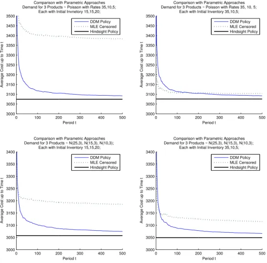
2.1 Comparison with parametric approaches. . . 48

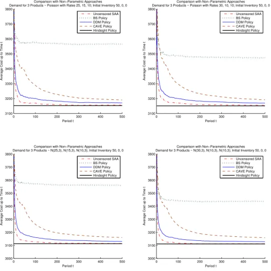
2.2 Comparison with nonparametric approaches. . . 49

2.3 Extreme cases with uneven lost-sales penalty costs. . . 50

3.1 Illustration of a target interval policy . . . 65

3.2 An illustration of a production cycle . . . 77

3.3 An illustration of the algorithmic design . . . 77

3.4 A schematic illustration of all possible scenarios . . . 84

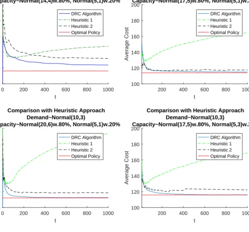
3.5 Computational performance of the DRC algorithm . . . 103

4.1 Illustration of the production cycles and dynamics of different policies 113 4.2 Illustration of the dynamics of our policy . . . 119

(9)

LIST OF TABLES

Table

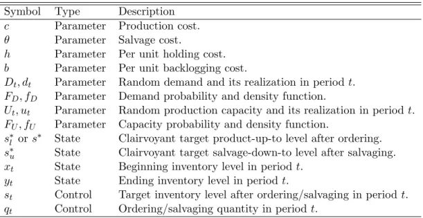
3.1 Summary of Major Notation . . . 64 4.1 Summary of Major Notation . . . 110 4.2 Summary of Computational Results . . . 138

(10)

ABSTRACT

The management of inventory and queueing systems lies in the heart of operations research and plays a vital role in many business enterprises. To this date, the majority of work in the literature has been done under complete distributional information about the uncertainties inherent in the system. However, in practice, the decision maker may not know the exact distributions of these uncertainties (such as demand, capacity, lead time) at the beginning of the planning horizon, but can only rely on realized observations collected over time. This thesis focuses on the interplay between learning and optimization of three canonical inventory and queueing systems, and proposes a series of first online learning algorithms.

The first system studied in Chapter II is the periodic-review multiproduct in-ventory system with a warehouse-capacity constraint. The second system studied in Chapter III is the periodic-review inventory system with random capacities. The third system studied in Chapter IV is the continuous-review make-to-stock M/G/1 queueing system. We take a nonparametric approach that directly works with data and needs not to specify any (parametric) form of the uncertainties. The proposed online learning algorithms are stochastic gradient descent type, leveraging the (some-times non-obvious) convexity properties in the objective functions. The performance measure used is the notion of cumulative regret or simply regret, which is defined as the cost difference between the proposed learning algorithm and the clairvoyant optimal algorithm (had all the distributional information about uncertainties been

(11)

given). Our main theoretical results are to establish the square-root regret rate for each proposed algorithm, which is known to be tight. Our numerical results also confirm the efficacy of the proposed learning algorithms.

The major challenges in designing effective learning algorithms for such systems and analyzing them are as follows. First, in most retail settings, customers typically walk away in the face of stock-out, and therefore the system is unable to keep track of these lost-sales. Thus, the observable demand data is, in fact, the sales data, which is also known as the censored demand data. Second, the inventory decisions may impact the cost function over extended periods, due to complex state transitions in the underlying stochastic inventory system. Third, the stochastic inventory system has hard physical constraints, e.g., positive inventory carry-over, warehouse capacity constraint, ordering/production capacity constraint, and these constraints limit the search space in a dynamic way.

We believe this line of research is well aligned with the important opportunity that now exists to advance data-driven algorithmic decision-making under uncer-tainty. Moreover, it adds an important dimension to the general theory of online learning and reinforcement learning, since firms often face a realistic stochastic sup-ply chain system where system dynamics are complex, constraints are abundant, and information about uncertainties in the system is typically censored. It is, therefore, important to analyze the structure of the underlying system more closely and devise an efficient and effective learning algorithm that can generate better data, which is then feedback to the algorithm to make better decisions. This forms a virtuous cycle.

(12)

CHAPTER I

Introduction

Supply chain management concerns the efficient allocation and control of raw ma-terials, finished products, and customer services. It plays a vital role in any successful business enterprise. The 2017 Annual State of Logistics Report shows that the total U.S. business logistics cost is 1.48 trillion, accounting for more than 7.7% of the U.S. gross domestic product (GDP). Among the decisions in supply chain management, inventory control is the first of mind and often the most critical component for any wholesale business. Indeed, the idea of inventory control not only applies to prod-ucts in the warehouse but also to seats on airplanes, beds in hospitals, drivers for ride-sharing companies, and so on. The goal for inventory control is to strike an optimal balance between under-stocking and over-stocking, i.e., maintaining a suffi-cient amount of inventory to fulfill customer demand while avoiding excess inventory taking up space in case of expiration, damage, or fund flow related problems. The key challenge lies in how to buffer the uncertainty of future evolution appropriately. Often firms find it hard to forecast the future demand, the unexpected interruption in the production phase, as well as the order or shipping lead time. Moreover, given nowadays complex business environment, firms often need to consider other impor-tant factors such as product correlations, strategic customers, and financial risks, when seeking the optimal policy.

(13)

Many of the theoretical optimization models in inventory and queueing control aim to capture the complexity of making decisions under uncertainty. In conventional models, the uncertainty about future evolution is usually defined through explicitly specified probability distributions or stochastic processes, which are treated as input data to respective optimization models. However, in most real-life applications, the true underlying distributions are not available or they are too complex to work with. Often, our knowledge is restricted to historical data, simulated data, or information from forecasting and market analysis. The objective of this thesis is to develop efficient and effective algorithms for sequential decision-making problems arising in the context of inventory and queueing control where the input data of the problems are unknown or uncertain at the beginning of the decision period. We aim to provide decision tools for decision-makers to better cope with uncertainty in these stochastic systems by absorbing, analyzing and utilizing data in an online fashion, which can be viewed as a substantial step to meet the challenges presented by the era of Big Data.

To achieve our goals, we will develop efficient and effective nonparametric learning algorithms that can simultaneously learn the input uncertainty in the underlying optimization problems as well as optimize the system-wide objective value on the fly. The algorithms compute policies based only on past observable data in an online manner. One major challenge in constructing such algorithms is that, in practice, the data or samples collected are often censored or inaccurate. For example, firms cannot typically observe their lost-sales since customers simply walk away when they find their desired items out of stock. As a result, the sales data collected are not true samples of demand, and the algorithmic design needs to correct such estimation biases in the long run. In our algorithmic framework, we take a non-parametric approach by not enforcing any parametric assumption on the underlying distributions. Our performance measure is regret-based, which quantifies the difference in objective values between our nonparametric sampling-based policy and the clairvoyant optimal

(14)

policy that has access to the true underlying distribution a priori. We will derive both theoretical performance guarantees as well as practical implementation strategies in this thesis. From the methodological point of view, the study of the algorithms will advance the understanding of the tradeoffs between learning and earning in the context of inventory and queueing systems, and the analysis will establish important connections with the general theory of online learning (which typically does not deal with inventory constraints and complex system dynamics).

1.1 Contributions of the Thesis

We study three different stochastic systems. We assume that the firm has no prior distributional information about the uncertainty, and must learn from past data. Our objective is to propose learning algorithms that admit provably tight regret.

In Chapter 2, we propose a nonparametric data-driven algorithm called DDM for the management of stochastic periodic-review multi-product inventory systems with a warehouse-capacity constraint. The demand distribution is not known a priori and the firm only has access to censored demand data. We measure the performance of DDM through regret, the difference between the total expected cost of DDM and that of an oracle with access to the true demand distribution acting optimally. We characterize the rate of convergence guarantee of DDM. More specifically, we show that the average expectedT-period cost incurred under DDM converges to the optimal cost at the rate of O(1/√T). We also discuss several extensions and conduct numerical experiments to demonstrate the effectiveness of our proposed algorithm.

In Chapter 3, we propose the first nonparametric learning algorithm for single-product, periodic-review, backlogging inventory systems with random production ca-pacity. Different than the current literature on this class of problems, we assume that the firm has neither prior information about the demand distribution nor the capac-ity distribution and only has access to past demand and supply data (which can be

(15)

referred to as censored capacity information). If both the demand and capacity dis-tributions are known at the beginning of the planning horizon, it is well-known that modified base-stock policies are optimal. When such distributional information is not available a priori to the firm, we propose a cyclic gradient-descent type of algorithm whose running average cost asymptotically converges to the clairvoyant optimal cost, where the clairvoyant optimal cost corresponds to the case where the firm knows the demand and capacity distributions and applies the optimal policy. We prove that the rate of convergence guarantee of our algorithm isO(1/√T), which is theoretically the best possible for this class of problems. We also conduct numerical experiments to demonstrate the effectiveness of our proposed algorithms.

In Chapter 4, we consider a canonicalM/G/1 make-to-stock queueing system that arises in many practical settings. The decision maker has no prior knowledge about the rate of the Poisson arrival process and the distribution of the production/service time, which must be learned over time from past observations. We propose a stochas-tic gradient descent algorithm and prove that its average expected cost converges to the clairvoyant optimal cost (had the arrival and service distributions been given) at a square-root convergence rate, which is provably tight for this class of problems. We also conduct numerical experiments to demonstrate the effectiveness of our proposed algorithms.

(16)

CHAPTER II

Nonparametric Algorithms for Multiproduct

Inventory Systems

2.1 Introduction

The study of stochastic multi-product inventory systems dates back to Veinott (1965). Most, if not all, of the papers on stochastic multi-product inventory systems assume that the stochastic future demand is given by a specific exogeneous random variable, and the inventory decisions are made with full knowledge of the future demand distribution. However, in practice, the demand distribution is usually not known a priori. Even with past demand data (often censored) collected, the selection of the most appropriate distribution and its parameters remains difficult (see Huh and Rusmevichientong (2009), Huh et al. (2011), Besbes and Muharremoglu (2013) for more discussions on censored demand in inventory systems).

Model overview and research issue. In our periodic-review multi-product lost-sales inventory system over a finite horizon of T periods, the demands across periods

t = 1, . . . T are (i.i.d.) random vectors Dt (with each component representing a

different product), respectively. There is a joint warehouse-capacity constraint M

imposed on the total number of products that can be held in inventory. The firm has no access to the true underlying demand distribution a priori, and can only observe

(17)

sales data (i.e., censored demand) over time. We develop a nonparametric data-driven adaptive inventory control policy π = (yt | t ≥ 1) where the decision yt represents

the order-up-to level in period t. We measure performance of our proposed policy

π through regret denoted by RT , C(π)− C(π∗), where C(π) is the total expected

cost ofπ and C(π∗) is the total expected cost of a clairvoyant optimal policy π∗ with access to the true underlying demand distribution a priori. The research question is to devise an effective nonparametric data-driven policy π that drives the average regret RT/T to zero with a fast convergence rate.

Main results and contributions. We propose a nonparametric data-driven algo-rithm called DDM for stochastic multi-product inventory systems with a warehouse-capacity constraint. We characterize the rate of convergence guarantee of DDM. More specifically, we show that the average regret RT converges to zero at the rate

of O(1/√T). Our algorithm DDM is a stochastic gradient descent type of algorithm, similar in spirit to Burnetas and Smith (2000), Kunnumkal and Topaloglu (2008) and Huh and Rusmevichientong (2009). The work closest to ours is Huh and Rus-mevichientong (2009) who studied an uncapacitated inventory system with a single product. The novelty of our work lies in both algorithmic design and performance analysis of DDM. First, unlike the uncapacitated single-product case, the gradient estimator in DDM could be sometimes indeterminable in the presence of a warehouse-capacity constraint on multiple products. Second, the projection step in DDM has to factor in both positive inventory carry-over of all products and the warehouse-capacity constraint. To maintain feasibility of the solution in each step, we solve two addi-tional optimization problems. The optimization problems can be efficiently solved by greedy algorithms, but the solution structure makes the asymptotic performance analysis invariably harder than that in the uncapacitated single-product case (where no optimization procedures are needed). The key technical challenge in our analysis is to derive an upper bound of the distance between the target order-up-to level and

(18)

the actual implemented order-up-to level (due to the warehouse-capacity constraint and positive inventory carry-over from previous periods). Note that the upper bound on this distance function is almost immediate in the uncapacitated single-product case while the development of an upper bound is significantly more complex in our multi-product setting. Third, we relate the inventory process to a GI/G/1 queue. We then develop a stochastic dominance argument and invoke a classical result on the expected busy period in GI/G/1 queue due to Loulou (1978).

We compare the computational performance of DDM with several existing para-metric and nonparapara-metric approaches in the literature. Our results show that DDM outperforms these benchmark algorithms in terms of both consistency and conver-gence rate. We also consider two interesting extensions, one with a more general warehouse-capacity constraint where different products may have different dimension or sizes, and the other one with discrete demand and order quantities.

Our work is relevant to the following research streams.

Multi-product stochastic inventory systems. There is a large body of litera-ture devoted to various classes of such problems. In this chapter, we focus our atten-tion on the classical stochastic multi-product inventory systems under a warehouse-capacity constraint, first studied by Veinott (1965). He provided conditions that ensure that the base-stock ordering policy is optimal in a periodic-review inventory system with a finite horizon. Subsequently,Ignall and Veinott (1969) showed that in the stationary demand case, a myopic ordering policy is optimal under certain mild conditions. Beyer et al. (2001, 2002) established the optimality of myopic policies in backlogged systems with separable costs by appealing to the sufficient condition provided by Ignall and Veinott (1969), which was further extended by Choi et al. (2005) under a relaxed demand assumption. Our work focuses on a nonparametric variant in which the demand distribution is not known a priori.

(19)

Nonparametric inventory systems. Burnetas and Smith(2000) developed a gra-dient descent type algorithm for ordering and pricing when inventory is perishable; they showed that the average profit converges to the optimal but did not establish the rate of convergence. Huh and Rusmevichientong (2009) proposed gradient de-scent based algorithms for lost-sales systems with censored demand. Subsequently, Huh et al. (2009) proposed algorithms for finding the optimal base-stock policy in lost-sales inventory systems with positive lead time. Huh et al. (2011) applied the concept of Kaplan-Meier estimator to devise another data-driven algorithm for cen-sored demand. Other nonparametric approaches in the inventory literature include sample average approximation (SAA) (e.g.,Kleywegt et al. (2002),Levi et al.(2007), Levi et al.(2015)) which uses the empirical distribution formed byuncensored samples drawn from the true distribution. Concave adaptive value estimation (e.g., Godfrey and Powell (2001),Powell et al.(2004)) successively approximates the objective cost function with a sequence of piecewise linear functions. The bootstrap method (e.g., Bookbinder and Lordahl (1989)) estimates the newsvendor quantile of the demand dis-tribution. The infinitesimal perturbation approach (IPA) is a sampling-based stochas-tic gradient estimation technique that has been used to solve stochasstochas-tic supply chain models (see, e.g.,Glasserman(1991)). Maglaras and Eren (2015) employed maximum entropy distributions to solve a stochastic capacity control problem. For parametric approaches, such as Bayesian learning (see, e.g., Lariviere and Porteus (1999), Chen and Plambeck (2008)) or operational statistics (see, e.g., Liyanage and Shanthikumar (2005),Chu et al.(2008)) in stochastic inventory systems, we refer readers toHuh and Rusmevichientong (2009) for an excellent discussion of the key differences between nonparametric and parametric approaches. This chapter contributes to the literature by studying multi-product inventory systems under a warehouse-capacity constraint, which is significantly more complex to analyze.

(20)

Online convex optimization. The aim of online convex optimization is to min-imize the cumulative loss function defined over a convex compact set with online learning process since the optimizer does not know the (convex) objective function a priori (see Hazan (2016), Shalev-Shwartz (2012) for an overview). Zinkevich (2003) has shown that the average T-period cost using a gradient descent based algorithm converges to the optimal cost at the rate of O(1/√T). This result was further ex-tended by Flaxman et al. (2005) in a bandit setting. Under additional technical assumptions, a modified algorithm by Hazan et al. (2006) achieves a faster conver-gence rate O(logT /T). Our problem differs from the conventional online convex optimization problems in that the target levels (or the iterates) may not be achieved due to policy-dependent dynamic inventory constraints.

Stochastic approximation. The proposed gradient descent type of algorithm also resembles the ones used in the Stochastic Approximation (SA) literature (see Ne-mirovski et al. (2009) and references therein), which should be carefully contrasted with ours. First, SA algorithms aim to solve a single-stage stochastic optimiza-tion problem by making successive experiments while the cost of experiments is ignored. On the other hand, our algorithm aims to minimize the cumulative loss suffered along the learning progress for a multi-stage closed-loop stochastic optimiza-tion problem. Putting into context, SA focuses on measuring the terminal regret E[Π(yT)−Π(y∗)], whereas our algorithm focuses on measuring the cumulative loss

over time_EhPT

t=1(Π(yt)−Π(y∗))

i

. Second, in the analysis of robust SA algorithms with general convex costs, the step size is chosen to be O(1/√t) to obtain a conver-gence rate ofO(1/√t) in the terminal regret criterion by appropriatelyaveraging the iterate solutions. The standard robust SA approaches cannot be adapted to our set-ting where the iterates cannot move “freely” due to policy-driven dynamic inventory constraints.

(21)

General notation. For any real vectors x,y ∈ _Rn_, _y _≥ _x _means

component-wise greater or equal to; x+ _{= (max{}_xi_,_0})n

i=1; |x| = (|xi|)ni=1; the join operator x∨y= (max{xi_{, y}i_})n

i=1; themeet operatorx∧y= (min{xi, yi})ni=1; for any integers

t and swith t≤s, x[t,s]=

Ps

j=txj andx[t,s)=

Ps−1

j=t xj;|| · || or|| · ||2 means 2-norm; || · ||1 means 1-norm. The notation, means “is defined as”.

2.2 Multi-Product Stochastic Inventory Systems

We consider a stochasticT-periodn-product inventory system under a warehouse-capacity constraintM (e.g.,Ignall and Veinott (1969),Beyer et al. (2001)). The firm has no knowledge of the true underlying demand distribution a priori, but can observe past sales data (i.e., censored demand data), and make adaptive inventory decisions based on the available information.

Random demand and regularity assumptions. For each periodt = 1, . . . , T and each producti= 1, . . . n, we denote the demand of producti in periodt by a random variable Di

t. For notational convenience, we use Dt = (D1t, . . . , Dtn) to denote the

random demand vector in period t, anddt= (d1t, . . . , dnt) to denote their realizations.

Assumption 2.1. We make the following assumptions and regularity conditions on demand.

(i). For each product i, Di

t is i.i.d. across time period t.

(ii). For each product i and for each period t, Di

t is independent (but not necessarily

identically distributed) of Dj

s for all j 6=i and s= 1, . . . , T.

(iii). For each product i and for each period t, Di

t is a continuous random variable

defined on a finite support[0, M], whose CDFFDi(·)is differentiable and density

F_D0i(x)>0 for all x∈[0, M].

(iv). For each product i and for each period t, _E[Di

(22)

Assumptions 2.1(a) and 2.1(b) assume some form of stationarity of demand, which is predominant in the nonparametric learning literature (see, e.g., Levi et al. (2007), Huh et al.(2009, 2011),Huh and Rusmevichientong (2009),Besbes and Muharremoglu (2013)). Assumption 2.1(c) ensures the per-period cost function defined in (2.3) is differentiable, finite-valued and strictly (jointly) convex, which guarantees a unique minimizer. Assumption 2.1(d) rules out degenerate demands.

System dynamics and objectives. Letft denote the information collected up to

the beginning of period t, which includes all the realized demands and past decisions. A feasible closed-loop policy π is a sequence of functions yt =πt(xt,ft),t = 1, . . . , T,

mapping beginning inventory xt and ft (state) into ending inventory yt (decision)

while satisfyingyt≥xt and the warehouse-capacity constraint (seeBertsekas (2000)

for discussions on closed-loop optimization problems). Note that when the demand distribution is known a prior, it suffices to consider policies of the form yt =πt(xt),

due to the assumed across-time independence of demands (see Bertsekas and Shreve (2007)).

Given a feasible policy π, we describe the sequence of events below. (Note that xπ

t,yπt andqπt’s are functions ofπ; for ease of presentation, we make their dependence

onπ implicit.)

(i). At the beginning of period t, the firm observes the starting inventory xt =

(x1_t, . . . , xn_t).

(ii). The firm decides to order qt = (qt1, . . . , qtn) ≥ 0, and the ending inventory

yt=xt+qt, whereyt= (yt1, . . . , ytn). We assume instantaneous replenishment.

The total inventory level is restricted by a warehouse-capacity constraint (see Ignall and Veinott (1969)), i.e.,

yt∈Γ, ( yt∈Rn+ : n X i=1 y_ti ≤M ) . (2.1)

(23)

(iii). The demand Dt is realized, denoted by dt, which is satisfied to the maximum

extent using on-hand inventory. Unsatisfied demand units are lost, and the firm only observes the sales quantity (or censored demand), i.e., min(di

t, yti)

for each product i in period t. The state transition can be written as xt+1 = (xt+qt−dt)+= (yt−dt)+.

(iv). The production, overage and underage costs at the end of period t is then c·qt+h·(yt−dt)++p·(dt−yt)+,wherec= (c1, . . . , cn),h= (h1, . . . , hn) and

p= (p1_{, . . . , p}n_{) are the per-unit purchasing, holding and lost-sales penalty cost}

vectors, respectively. We note that the cost minimization model with lost-sales assumes thatp≥c(seeZipkin (2000)) since the firm loses revenue and goodwill from the sale and the revenue has to be greater than the production cost. (Our approach also works for time-invariant random purchasing cost vector.)

Assuming the salvage value of any left-over product at the end of planning horizon equals its production cost, the total expected cost incurred by π can be written as

C(π) = _E " _T X t=1 c·(yt−xt) +h·(yt−Dt)++p·(Dt−yt)+ # −_E[c·xT+1], = −c·x1+ T X t=1 Ec·yt+ (h−c)·(yt−Dt)++p·(Dt−yt)+ , (2.2)

where the second equality follows from xt+1 = (yt−dt)+ and some simple algebra.

If the underlying distribution Dt is given a priori, the stochastic inventory control

problem specified above can be formulated using dynamic programming (see Beyer et al.(2001)) with state variablesxt, control variablesyt(with xt ≤yt∈Γ), random

disturbancesDt, and state transitionxt+1 = (yt−dt)+. It turns out that this problem

is in fact “myopically” solvable, which is discussed next.

Clairvoyant optimal policy. We first characterize the clairvoyant optimal policy where the distribution of Dt is known a priori. We define Π(·) to be the per-period

(24)

expected cost function, Π(a) = Πt(a),E c·a+ (h−c)·(a−Dt)++p·(Dt−a)+ . (2.3)

Lety∗ be a unique critical (deterministic) vector defined by

y∗ _,arg min

a∈Γ:a≥0Π(a). (2.4)

Theorem 2.2. Under Assumption 2.1, when the demand distribution is known a priori, ordering up to y∗ defined in (2.4) in each period is optimal, with expected per-period cost Π(y∗).

Proof. Based on (2.3), we define amyopic feasible (closed-loop) policy ¯πas a sequence of functions ¯yt = ¯πt(xt), t = 1, . . . , T, mapping beginning inventory (state) xt into

ending inventory (decision) ¯yt, which also “myopically” minimizes per-period cost

Πt(·) with beginning inventory xt, i.e.,

¯

yt(xt),arg min

a∈Γ:a≥xt

Πt(a). (2.5)

The above feasible policy ¯π is myopic, because it only optimizes per-period cost in each period (the immediate reward). This is in contrast with standard dynamic programming or approximate dynamic programming approaches. To ease the presen-tation of establishing optimality of ¯π, following Ignall and Veinott (1969), we keep xt, ¯yt, Πt time-generic, i.e.,

¯

y(x)_,arg min

a∈Γ:a≥xΠ(a). (2.6)

It is important to see that ¯y(x) is the unique minimizer of (2.6), due to Assumption 2.1 ensuring strict (joint) convexity of Π(y) over the feasible region, and the fact that

(25)

the constraint set is affine (see Boyd and Vandenberghe (2004)).

Lemma 2.3. The optimization problem defined in (2.6)has a unique minimizery(x).¯ Proof. Due to Assumption 2.1, the cost function Π(·) is differentiable and finite-valued. The derivatives inside expectation are bounded, and also the expectation is a multiple integration over finite ranges. Hence this guarantees the validity of interchange between differentiation and expectation.

Next we argue that Π(·) are strictly (jointly) convex over the feasible region. For alli and j, ∂2_Π(a) ∂(ai₎2 = (h i₊_pi ₋_ci₎_F0 Di(ai)>0; ∂2_Π(a) ∂ai_∂aj = 0,

where Assumption 1(c) ensures F_D0 i(ai) > 0 for all ai ∈ [0, M]. Hence, the Hessian

matrix is positive definte (with all strictly positive eigenvalues) over the entire feasible region, ensuring Π to be strictly (jointly) convex.

Now consider the optimization problem (with a given starting inventoryx) defined in (2.6). Since Π(y) is strictly (jointly) convex and the constraint set is affine, ¯y(x) is the unique minimizer. (See Boyd and Vandenberghe (2004) for discussions of unique minimizer in convex optimization problems and also Example 5.4.).

Next we shall show that the myopic policy ¯π defined above is optimal. Ignall and Veinott (1969) provided a sufficient condition calledsubstitute property (together with two mild regularity assumptions) under which the myopic policy is optimal.

Definition 2.4 (Substitute property). For any inventory levels x,˜x∈Γ,

if x≥˜x, then ¯y(x)−x≤y(˜¯ x)−˜x.

Definition 2.5 (Regularity conditions in Ignall and Veinott (1969)). The two reg-ularity conditions in Ignall and Veinott (1969) are: (a) x ≤ x0 ≤ y(x) implies¯

(26)

¯

y(x) = ¯y(x0) for x,x0 ∈ Γ; (b) The state transition permits either pure, partial, or no backlogging (lost-sales).

The regularity condition (a) is satisfied by ¯y(x) being the unique minimizer of (2.6) by Lemma 2.3, and the regularity condition (b) is immediate since we consider a standard lost-sales model.

We can now proceed to establish the optimality of myopic policies for the multi-product lost-sales system by showing that the sufficient condition (substitute prop-erty) given above holds for our system.

Proposition 2.6. Under Assumption 2.1, when the demand distribution is known a priori, the myopic ordering policy defined in (2.5) is optimal for the multi-product lost-sales inventory systems.

To prove Proposition 2.6, we need to derive several important properties of the myopic policy. Now consider the two possible starting inventory levels xand ˜x, with x ≥ ˜x. For notational (superscript) convenience, we use θ instead of y∗ to be the global minimizer of Π(·) over Γ. Recall that θ =y∗ _,arg mina∈ΓΠ(a), and also the myopic order-to-up level ¯y(x) _, arg mina∈Γ:a≥xΠ(a). For simplicity, we define the boundary of our warehouse storage constraint,

∂Γ_, ( y∈_Rn₊ : n X i=1 yi =M ) .

Note that y ∈ ∂Γ means that the total order-up-to levels have reached the total storage limit M. If y∈/∂Γ, then the warehouse storage constraint is not tight.

Now denote the jth _{partial derivative of Π(·) by Π}0

j(·). We then develop some

useful properties of the myopic order-up-to levels ¯y(·).

Lemma 2.7. Let x∈Γ and θ be the global minimizer of Π(·) over Γ, (i). xj ≥θj ⇒y¯j(x) =xj.

(27)

(ii). xj _≤_θj _⇒_y_¯j_(x)_≤_θj_.

Proof. The proof is straightforward. Statement (i) holds becausexj _≥_θj _{(the starting}

inventory is higher than the global minimizer) for productj, it is sub-optimal to order any more product j. Statement (ii) holds because ifxj _≤_θj _{(the starting inventory}

is lower than the global minimizer), it is sub-optimal to raise the inventory above the global minimizer.

Lemma 2.8. Let x∈Γ and θ be the global minimizer of Π(·) over Γ, (i). θ ∈∂Γ⇒y(x)¯ ∈∂Γ;

(ii). y(x)¯ ∈/ ∂Γ, xj _≤_θj _⇒_y_¯j_{(x) =}_θj_.

In Lemma 2.8, statement (i) states that if the global minimizer occupies the entire storage space, then the myopic order-up-to levels will also occupy the entire storage space. This is because our myopic policy will always order as much as possible to approach the global minimizer. Statement (ii) states that if the total myopic order-up-to level has not reached the storage limit M, then if xj _≤ _θj_{, the myopic policy}

will raise inventory level for productj to the global minimizer θj_.

Proof. We prove (i) by contradiction. Suppose that θ ∈∂Γ and ¯y(x)∈/ ∂Γ, then

n X i=1 θi =M and n X i=1 ¯ yi(x)< M.

It is obvious that there exists at least one j such that ¯yj_(x)_{< θ}j_{. Since} _θ _minimizes

Π(·) over Γ, it is clear that θ either reaches the global minimizer of Π(·) over the entire real line _Ror is smaller than it due to the storage constraint, so the derivative Π0_j(θ)≤0.Therefore, since Π(·) is strictly convex,

(28)

On the other hand, since ¯y(x)∈/ ∂Γ and ¯y(x) is a minimizer of Π(·) over set{y|y≥ x,y ∈ Γ}, it is clear that ¯y(x) either reaches θ or is greater than it because of the initial on-hand inventory, so Π0_j(¯y(x))≥0, which results in a contradiction, thereby proving (i).

To prove (ii), we observe from the contraposition of (i), i.e., ¯y(x)∈/ ∂Γ⇒θ /∈∂Γ. Then for any product j, ¯yj(x) is not restricted by the storage constraint, and thus if θj ≥xj, then θj can always be reached, implying that ¯yj(x) = θj. This completes the proof.

Lemma 2.9. y¯j_(x)_{> x}j _⇒_Π0

j(¯y(x)) = miniΠ0i(¯y(x))

Lemma 2.9 states that if a product is ordered, then the marginal cost of any additional ordering must be equal across the products. Intuitively, if the marginal cost of ordering this product is higher than others, we can always reduce the quantity of this product and order more of the other products. The rigorous proof is as follows. Proof. We prove this result by contradiction. Suppose that there exists an i, 1 ≤

i ≤ n, such that Π0_i(¯y(x)) < Π0_j(¯y(x)). Then, for a sufficiently small > 0, (¯y1(x), ...y¯j(x)−, ...,y¯i(x) +, ...,y¯n(x))∈Γ, and we have

Π(¯y(x))−Π(¯y1(x), ...y¯j(x)−, ...,y¯i(x) +, ...,y¯n(x)) = (Π0_j(¯y(x))−Π_i0(¯y(x))) +o(2)>0,

which contradicts to the fact that ¯y(x) minimizes Π(·) over set{y|y≥x,y∈Γ}. Now, we are ready to prove Proposition 2.6.

Proof. To establish the optimality of myopic policies for the multi-product lost-sales system, it suffices to verify that the substitute property (2.4) holds, i.e., for any inventory levelsx,˜x∈Γ, ifx≥x, then ¯˜ y(x)−x≤y(˜¯ x)−˜x.

(29)

We know that the myopic order-up-to levels ¯yj_(x)_≥_xj _{for any product}_j _if_x_∈_Γ.

Similarly, ¯yj_(˜_x)_≥_x_˜j _{for any product} _j _if _˜_x_∈_{Γ. Now if ¯}_yj_{(x) =} _xj_{, then we have}

0 = ¯yj(x)−xj ≤y¯j(˜x)−x˜j.

Thus, it suffices to prove that ¯yj_(x) _≤ _y_¯j_(˜_{x), whenever ¯}_yj_(x) _{> x}j_{. We have to}

consider three cases as follows.

Case (a). First, if both ¯y(x)∈/ ∂Γ and ¯yj_(˜_x) _∈_/ _∂_{Γ, then it follows from Lemma}

2.7 and Lemma 2.8 that

¯

yj(x) = max{θj, xj}, y¯j(˜x) = max{θj,x˜j}, ∀j.

Then ¯yj_{(x) = ¯}_yj_(˜_{x) and the result follows immediately.}

Case (b). Second, if ¯y(x) ∈ ∂Γ but ¯yj_(˜_x) _∈_/ _∂_{Γ, then by Lemma 2.7 (ii) and}

Lemma 2.8 (ii), we have ¯yj(x)≤θj = ¯yj(˜x), and the result also follows immediately. It is impossible for the case where ¯y(x)∈/ ∂Γ and ¯yj(˜x)∈∂Γ to happen. To see this, if such case exists, then we can always find somej such that forxj >x˜j, ¯yj(˜x)>y¯j(x). However, by Lemma 2.7 (ii) and Lemma 2.8 (ii), we know that ¯yj_(x)_≤ _θj _{= ¯}_yj_(˜_x)_,

which results in a contradiction.

Case (c). Third, we need to analyze the remaining case where ¯y(x) ∈ ∂Γ and ¯ yj_(˜_x)_∈_∂_{Γ, i.e.,} n X j=1 ¯ yj(x) = n X j=1 ¯ yj(˜x) =M. (2.7)

We partition all the products into three sets as follows,

Ia ={k : ¯yk(x)> xk}, Ib ={k : ¯yk(x) =xk∩Π0_k(¯yk(x)≤0}, Ic ={k : Π0_k(¯yk(x)>0}.

Note that these three sets are disjoint and the union of them is exhaustive.

(30)

By Lemma 2.7, it is clear that ¯yj_(˜_x)_≤_max{˜_xj_{, θ}j_{}. Hence, ¯}_yj_(˜_x)₋_y_¯j_(x)_≤_{0 for all}

j ∈Ic_{. Together with (2.7), we know that} n

X

j∈Ia_∪_Ib

¯

yj(˜x)−y¯j(x)≥0.

If ¯ym_(˜_{x) = ¯}_ym_{(x) for all}_m_∈_Ia_∪_Ib_{, then the result follows immediately. Now consider}

the case where there exists a product m ∈ Ia_∪_Ib _{such that ¯}_ym_(˜_x) _> _y_¯m_{(x). This}

implies that ¯ym_(˜_x)_> _y_¯m_(x) _≥ _xm _≥ _x_˜m _≥ _{0. By Lemma 2.9, we have Π}0

m(¯y(˜x)) =

miniΠ0i(¯y(˜x)). Moreover, due to the strict convexity of Π(·), then we have

min i Π 0 i(¯y(˜x)) = Π 0 m(¯y(˜x))>Π 0 m(¯y(x)). (2.8)

To complete the proof, it suffices to show that for any product j ∈ Ia_{, ¯}_yj_(˜_x) _≥

¯

yj_{(x). Now suppose there exists a product} _n _∈ _Ia _{such that ¯}_yn_(˜_x) _< _y_¯n_{(x). It is}

clear that ¯yn_(x) _> _y_¯n_(˜_x) _≥ _{0. By Lemma 2.9, we have Π}0

n(¯y(x)) = miniΠ0i(¯y(x)).

Moreover, due to the strict convexity of Π(·), then we have

min i Π 0 i(¯y(x)) = Π 0 n(¯y(x))>Π 0 n(¯y(˜x)). (2.9)

Note that (2.8) implies that Π0_n(¯y(˜x))>Π0_m(¯y(x)) but (2.9) implies that Π0_m(¯y(x))>

Π0_n(¯y(˜x)), which results in a contradiction. This completes the proof. Equipped with Proposition 2.6, we are ready to prove Theorem 2.2.

Proof. Proposition 2.6 fully characterizes the structural properties of optimal policies as follows. Lety∗ be a unique critical (deterministic) vector defined by in (2.4). Then a clairvoyant optimal policyπ∗ is characterized as follows:

(i). If the beginning inventory level of product i is above its individual base-stock level (i.e., the ith component of y∗), then this product is not ordered in the

(31)

period.

(ii). If this product i is ordered in the period, the ending inventory level (after ordering) does not exceed its individual base-stock level (i.e., theith _component

of y∗).

(iii). If there is enough storage space to bring all products (whose inventory levels are below their individual base-stock levels) up to their base-stock levels, then such an order is optimal. Otherwise, the ending inventory levels takes up all the available storage space.

Thus, the stationary multi-period inventory problem is analytically equivalent to the single-period problem, and ordering up to y∗ in each period is also optimal for this problem. Clearly, once we start below y∗, and order up to y∗, we remain at or below y∗ thereafter; in such a case, the expected cost incurred in each period is Π(y∗).

2.3 Nonparametric Data-Driven Inventory Control Policies

When the firm has no knowledge of the true underlying distribution ofDta priori,

we aim to find a provably good adaptive data-driven inventory control policy that makes the total expected system costs close to the optimal strategy. The proposed data-driven algorithm DDM maintains a vector triplet of sequences (zt,yˆt,yt)t≥0. The first sequence (zt)t≥0 represents the constraint-free target inventory levels where the warehouse storage constraint is waived. The second sequence (ˆyt)t≥0 represents the target inventory levels when the warehouse storage constraint is taken into account. However, the target inventory levels (ˆyt)t≥0 may not be always feasible due to ware-house capacity constraint and positive inventory carry-over. Thus, we use the third sequence (yt)t≥0 to represent theactual implemented inventory levels after ordering. We first present a compact description of our data-driven multi-product algorithm (DDM).

(32)

Data-Driven Multi-product Algorithm (DDM).

Step 0. (Initialization.) Set the initial inventory levelsy0 = ˆy0 =z0 to be any values within Γ and then set the initial values t = 0, τ0 = 0 and k = 0.

For each period t= 0, . . . , T −1, repeat the following steps:

Step 1. (Setting the constraint-free and constrained target inventory levels.)

Case 1: If yt ≥ ˆyt (i.e., yti ≥ yˆti for all i = 1, . . . , n), the algorithm updates the

constraint-free target inventory levelszt+1 by

zt+1 = ˆyt−ηtGt(ˆyt), (2.10) whereηt = γM √ n·maxi{pi−ci, hi} 1 √ t for some γ >0

for each product i= 1, . . . , n, and the ith _{component of} _G

t is defined as Gi_t(ˆyt) =        hi_, _{if ˆ}_yi t > dit, −(pi₋_ci₎_, _{if ˆ}_yi t ≤dit. (2.11)

Note thatγ = 1 for achieving the tightest theoretical bound.

Then the algorithm sets the constrained target inventory levels ˆyt+1 by solving

ˆ

yt+1 = arg min

w∈Γ||w−zt+1||2. (2.12) Record the break point τk :=t and increase the value k by 1.

Case 2: Else if yt ˆyt (i.e., there exists an i such that yti < yˆti), the algorithm

keeps both the constraint-free and constrained target inventory levels unchanged, i.e., zt+1 =zt and yˆt+1 =yˆt.

(33)

Define the set J and its complement as

J _,i:xi_t₊₁ >yˆ_ti₊₁ , J¯_,i:xi_t₊₁ ≤yˆ_ti₊₁ . (2.13)

For each product i∈J, we set the actual implemented levels

y_ti₊₁ =xi_t₊₁, if xi_t₊₁ >yˆ_ti₊₁. (2.14)

If ¯J 6=∅, then we set the actual implemented levelsyt+1 by solving

minX i∈_J¯ (ˆyi_t₊₁−yi_t₊₁)2 s.t. X i∈_J¯ y_ti₊₁ ≤M −X j∈J xj_t₊₁, y_ti₊₁ ≥xi_t₊₁, ∀i∈J .¯(2.15)

This concludes the description of the algorithm.

2.3.1 Algorithm Overview of DDM and Properties

Step 1: (Stochastic Gradient Descent). LetT ={τ0, τ1, . . . , τm}with τm ≤T,

which is the set of break points of DDM. In each period τk+ 1 (k = 1, . . . , m), we

update the constraint-free target levels zt+1 by a stochastic gradient descent step. Conceptually, we update the minimizer along the negative direction of the true gradi-ent of Π(·). However, since the true cost function Π(·) is not available to us (without knowing the underlying demand distribution), we can only rely on the observed sales data dt to provide us an estimator of the true gradient of Π(ˆyt) at the points yˆt.

The estimator Gi_t(ˆyt) defined in (2.10) can be computed using the sales (censored

demand) data observed by the firm in period t ∈ T. When t ∈ T, we have yi t ≥ yˆti

for all i = 1, . . . , n. Hence, the event {ˆyi

t ≤ dit} is equivalent to the case where the

ending inventory in periodtis at mostyi

t−yˆit, which is an observable event; the event

{ˆyi

t > dit} is equivalent to the case where the ending inventory in period t is strictly

(34)

an unbiased estimator of the true gradient ∇Π(ˆyt) at yˆt, i.e., E[Gt(ˆyt)] = ∇Π(ˆyt),

where the expectation is taken over the demand in periodt. On the other hand, when

t /∈ T,Gi

t(ˆyt) may beindeterminable because the actual implemented inventory levels

could fall below the target order-up-to levels. To be more specific, when yi

t <yˆti and

yi

t≤dt, the firm only observes the stockout but not the lost-sales quantity. Therefore,

the firm cannot distinguish between y_ti ≤dt<yˆti and yit<yˆit≤dt, and hence cannot

determine the value ofGi_t(ˆyt). In periods whent /∈ T, we keep the target order-up-to

levels unchanged.

We then carry out a greedy projection of the constraint-free target inventory levels zt+1 onto the warehouse storage constraint set Γ via (2.12), more specifically,

min n X i=1 (ˆyi_t₊₁−z_ti₊₁)2 s.t. n X i=1 ˆ y_ti₊₁ ≤M, yˆ_ti₊₁ ≥0, ∀i. (2.16)

We also make two simple observations that will be useful in Section 2.4. (a) A simple observation leads to the lower and upper bounds of z_ti₊₁ for each product

i, i.e., ˆy_ti − ηthi ≤ zti+1 ≤ yˆti +ηt(pi −ci). In fact, zti+1 has to hit one of the two boundaries. (b) Another important observation is that when the product i in the first step updates its constraint-free target levelzi

t+1 through a positive direction, i.e.,

zi

t+1 = ˆyti +ηt(pi −ci) ≥ yˆit ≥ 0, we must have ˆyit+1 ≤ zit+1. To see this, suppose otherwise ˆyi

t+1 > zti+1, we can decrease ˆyit+1 to zti+1, thereby strictly improving the objective value of (2.16) while maintaining feasibility. On the other hand, when the product i in the first step updates its constraint-free target level z_ti₊₁ through a negative direction, we have z_ti₊₁ = ˆy_ti −ηthi ≤ yˆit, Thus, this leads to the following

property that will be useful in the performance analysis,

ˆ

yi_t₊₁ ≤yˆ_ti+ηt(pi−ci), ∀i= 1, . . . , n. (2.17)

(35)

in the second step may not be achievable or implementable, due to the physical inventory carry-over and the warehouse capacity constraint. We then need to carry out an additional optimization procedure as follows. This step tries to order as many products as possible to reach the target level, and it is easy to solve quantitatively but hard to analyze. First we divide all the products into two groups, namely, the setJ and its complement as defined in (2.13). We then have the following two cases. Case 1. For each product i∈ J, i.e., the beginning inventory level of product i

is already greater than its target level. It is natural to not order any more product i

and hence we follow (2.14).

Case 2. Now we focus on the set ¯J 6=∅. Since the remaining inventory space now becomes M −P

j∈Jx

j

t+1,we solve the optimization problem (2.15) to determine the actual implemented levels yt+1. Note that the optimization problem is well-defined since M −X j∈J xj_t₊₁ =M −X j∈J (yj_t −dj_t)+≥M −X j∈J y_tj ≥0,

where the inequality follows from the fact that the algorithm keeps yt ∈Γ.

The optimization (2.15) attempts to raise our inventory level as close as possible to the target inventory level ˆy_ti₊₁ for each product i∈J¯; however, it is possible that some of the products in ¯J cannot hit the target level due to inventory constraints. Since we minimize the 2-norm type of objective function, it can be readily verified that the optimization (2.15) makes the shortfalls defined as ˆyi

t+1 −yti+1 as even as possible across the products in the set ¯J.

Note that if the optimal objective value of (2.15) is equal to 0, then the algorithm goes to Case 1 in the next period and updates the target inventory levels. Otherwise it goes to Case 2 and maintains the target inventory levels; while maintaining these target levels, the inventory levels within J are decreasing and more inventory space is freed over time, and the shortfalls will decrease to zero.

(36)

2.4 Performance Analysis of DDM

The regret of our data-driven algorithm, denoted byRT, is defined as the difference

between the optimal clairvoyant cost (given the demand distribution a priori) and the cost incurred by our data-driven algorithm (which learns the demand distribution over time). That is, for any T ≥1,

RT ,E " _T X t=1 Π(yt) # − T X t=1 Π(y∗),

whereytare the actual implemented order-up-to levels of our nonparametric

(closed-loop) algorithm DDM, and y∗ is the clairvoyant optimal solution in (2.4). Theorem 2.10 below states the main result in this chapter.

Theorem 2.10. Under Assumption 2.1, the average regret RT/T of our data-driven

algorithm DDM approaches0at the rate of1/√T. That is, there exists some constant

K, such that for any T ≥1, 1 TRT , 1 TE " _T X t=1 Π(yt) # −Π(y∗)≤ √K T,

whereyt are actual implemented order-up-to levels of our nonparametric (closed-loop)

algorithm DDM, and y∗ is the clairvoyant optimal solution in (2.4).

It is known that in the general convex case (without assuming smoothness and strong convexity), this rate of O(1/√T) is unimprovable (see, e.g., Theorem 3.2. of Hazan (2016)). Our key contribution here is to establish this best possible rate even with inventory and capacity constraints (i.e., the iterates cannot move “freely” due to policy-driven dynamic inventory constraints).

Then the proof of Theorem 2.10 is the direct consequence of the following two key lemmas.

(37)

Lemma 2.11. For any T ≥1, there exists a constant K1 ∈R such that ∆1(T) =_E " _T X t=1 Π(ˆyt)− T X t=1 Π(y∗) # ≤K1 √ T ,

where ˆyt are target order-up-to levels of DDM, and y∗ is the clairvoyant optimal

solution in (2.4).

Lemma 2.12. For any T ≥1, there exists some constant K2 ∈R such that

∆2(T) =E " _T X t=1 Π(yt)− T X t=1 Π(ˆyt) # ≤K2 √ T ,

where yt andyˆt are actual implemented and target order-up-to levels of DDM,

respec-tively.

2.4.1 Bound on ∆1 - Online Convex Optimization (Proof of Lemma 2.11) The proof of Lemma 2.11 builds upon the ideas and techniques used in online convex optimization (see, e.g., Zinkevich (2003) and Flaxman et al. (2005)). It is shown the cost function Π(·) is jointly convex, andG(·) is an unbiased estimator of the true expected gradient of Π(·) under censored demand within the set of breakpoints. In addition, this gradient estimator is bounded, i.e.,||G(·)||2

2 ≤n(maxi{pi−ci, hi})2.

Proof. Due to convexity of the cost function Π(y), we have

E[Π(ˆyt)−Π(y∗)]≤E[∇Π(ˆyt)(ˆyt−y∗)]. (2.18)

Note that the subgradient∇Π(ˆyt) defines the supporting hyperplane of Π at the point

ˆ yt.

For any period t ∈ T, i.e., in the set of break points, we can obtain the upper bound of the second moment difference between our target inventory level and the

(38)

optimal target inventory level. E||ˆyt+1−y∗||2 ≤ E||zt+1−y∗||2 (2.19) = _E||ˆyt−ηtGt(ˆyt)−y∗||2 = _E||ˆyt−y∗||2+η2tE||Gt(ˆyt)||2−2ηtE[Gtn(ˆyt)(ˆyt−y ∗ )],

where the first inequality follows the optimization (2.12) and the Pythagorean The-orem since

||zt+1−y∗||2 =||ˆyt+1−y∗||2+||zt+1−ˆyt+1||2

by property of the 2-norm projection; the first equality follows from the definition of zt+1; the second equality follows from a simple binomial expansion.

We can also re-write _E[Gt(ˆyt)(ˆyt−y∗)] by taking conditional expectation on the

value ofyˆt,

E[Gt(ˆyt)(ˆyt−y∗)] = E[E[Gt(ˆyt)(ˆyt−y∗)|ˆyt]] (2.20)

= _E[_E[Gt(ˆyt)|ˆyt] (ˆyt−y∗)]

= _E[∇Π(ˆyt)(ˆyt−y∗)],

where the first equality holds because y∗ does not relate with yˆt; the last equality

follows from the fact that Gt is an unbiased estimator of the true gradient ∇Π.

Combining (2.19) and (2.20), it is clear that

E[∇Π(ˆyt)(ˆyt−y∗)]≤ 1 2ηt E ||ˆyt−y∗||2−E||ˆyt+1−y∗||2 +ηt 2E||Gt(ˆyt)|| 2 . (2.21)

(39)

construction of DDM, E " _T X t=1 Π(ˆyt)− T X t=1 Π(y∗) # = _E "_k₋₁ X s=0 τs+1 X t=τs+1 (Π(ˆyt)−Π(y∗)) # ≤ M l ·E " _k X s=1 (Π(ˆyτs)−Π(y ∗ )) # ,

where the inequality follows from the fact that the time between any two consecu-tive break points cannot exceed the time for a “fictitious” system with M inventory units for each product i = 1, . . . , n to become empty along every sample path. The expectation of the latter (which is independent of ˆyt) is upper bounded by M/l.

It then suffices to bound the term _EhPk

s=1(Π(ˆyτs)−Π(y

∗₎₎i_{. Now, by summing}

both sides of (2.18) over periods τ1 to τk,

E " _k X s=1 (Π(ˆyτs)−Π(y ∗ )) # ≤ k X s=1 E[∇Π(ˆyτs)(ˆyτs −y ∗ )] (2.22) ≤ k X s=1 1 2ητs E||ˆyτs −y ∗_||2₋ E||ˆyτs+1−y ∗_||2 + ητs 2 E||Gτs(ˆyτs)|| 2 = k X s=1 1 2ητs E||ˆyτs −y ∗_||2₋ E||ˆyτs+1 −y ∗_||2 +ητs 2 E||Gτs(ˆyτs)|| 2 = 1 2ητ1 E||ˆyτ1 −y ∗_||2₋ 1 2ητk E||ˆyτk+1−y ∗_||2₊1 2 k X s=2 1 ητs − 1 ητs−1 E||ˆyτs−y ∗_||2 + k X s=1 ητs E||Gτs(ˆyτs)|| 2 2 ≤ 2M2 1 2ητ1 +1 2 k X s=2 1 ητs − 1 ητs−1 ! +n(maxi{p i₋_ci_{, h}i_})2 2 k X s=1 ητs = M 2 ητk +n(maxi{p i₋_ci_{, h}i_})2 2 k X s=1 ητs,

where the first and second inequalities follows from (2.18) and (2.21), respectively; the first equality holds since yˆτs+1 = yˆτs+1 by the construction of DDM; the last

(40)

inequality follows from the fact that for anyx,y∈Γ, ||x−y||2 2 ≤ ||x|| 2 2+||y|| 2 2 ≤ ||x|| 2 1+||y|| 2 1 ≤2M 2_.

Putting everything together, we have

E " _T X t=1 Π(ˆyt)− T X t=1 Π(y∗) # ≤ M l M2 ηT + n(maxi{p i ₋_ci_{, h}i_})2 2 k X s=1 ητs ! . (2.23)

Note that we have chosen our step size “optimally” as

ηt= γM √ n·maxi{pi−ci, hi} 1 √ t for some γ >0, so that k X s=1 ητs ≤ T X t=1 ηt = γM √ n·maxi{pi−ci, hi} T X t=1 1 √ t ≤ γM √ n·maxi{pi−ci, hi} 2√T . (2.24)

Plugging (2.24) and ηT into (2.23) yields the result with the constant term

K1 = (γ +γ−1)M2l−1 √

n·max

i {p

i ₋_ci_{, h}i_}_.

Note that putting γ = 1 gives the tightest bound. This completes the proof.

2.4.2 Bound on ∆2 - Stochastic Dominance and a GI/G/1 Queue (Proof of Lemma 2.12)

The main focus of this chapter is to establish the result in Lemma 2.12. First we derive a bound of the gap between the cost functions associated with the actual

(41)

implemented level yt and the desired target level ˆyt, using the distance function

|yt−ˆyt|.

Lemma 2.13. The difference in cost functions

E[Π(yt)−Π(ˆyt)]≤E[(h∨(p−c))· |yt−yˆt|].

Proof. By the definition of the per-period cost function in (2.3), it follows that

E[Π(yt)−Π(ˆyt)] ≤ E[c·(yt−yˆt)] +E (h−c)·(yt−yˆt)+ +_Ep·(ˆyt−yt)+ = _Eh·(yt−yˆt)+ +_E(p−c)·(ˆyt−yt)+ ≤ _E[(h∨(p−c)· |yt−yˆt|],

where the last inequality follows from various operators defined at the end of Section 1.

Given Lemma 2.13, we need to develop an upper bound on the distance function |yt −yˆt|, which is the crux of our performance analysis. Lemmas 2.14 and 2.15

below play a major role in the development of such an upper bound. Their proof strategy relies heavily on the construction of DDM and also the structural properties of optimization problems (2.15) and (2.16), which is quite involved.

Lemma 2.14 below provides an upper bound on the distance function for products in the set J in which the beginning inventory level already exceeds the target order-up-to level.

Lemma 2.14. In each period t+ 1, we bound the distance function for all i ∈ J _, i:xi t+1 >yˆti+1 . X i∈J |y_ti₊₁−yˆ_ti₊₁| ≤X i∈J y_ti−yˆ_ti+η_t   X i∈J hi+X j∈_J¯ pj−cj  − X i∈J di_t.

(42)

Proof. Case 1. We first consider time period t ∈ T = {τ0, . . . , τk}, which belongs

to the set of break points in DDM. Due to the construction of DDM, we update the target levels at t+ 1 only if t∈ T. For each product i∈J, i.e., xi

t+1 >yˆti+1, we have

yi

t+1 = xit+1 > yˆit+1 ≥ 0 by (2.14). This implies that yti+1 > 0, and by the lost-sales system dynamics, we have

xi_t₊₁ = (yi_t−dt)+=yti−dt >0. (2.25)

The next key step is to compare the target level ˆyi

t+1 with the constraint-free target level zi

t+1. First, notice that when yti − dit > 0, the algorithm updates the

constraint-free target level in a negative direction, i.e.,

z_ti₊₁ = ˆy_ti−ηthi <yˆti. (2.26)

Second, by the important property (2.17) of our algorithm, we have

ˆ

y_tj₊₁ ≤yˆ_tj+ηt pj −cj

, ∀j = 1, . . . , n.

Thus, the maximum positive displacement ofyˆt+1 fromˆyt (excluding the set J) is

X j∈J¯ ˆ y_tj₊₁−yˆ_tj ≤ X j∈J¯ ηt pj−cj . (2.27)

Now, to draw a relation between ˆyi

t+1 and zti+1, there are two cases. Subcase 1a. In the first case where Pn

j=1yˆ j t+1 ≥ Pn j=1yˆ j t, we must have X i∈J z_ti₊₁−yˆ_ti₊₁ <X i∈J ˆ y_ti−yˆ_ti₊₁≤X j∈_J¯ ˆ yj_t₊₁−yˆj_t ≤ X j∈_J¯ ηt pj−cj ,(2.28)

(43)

Pn j=1yˆ j t+1 ≥ Pn j=1yˆ j

t; and the third inequality follows from (2.27).

Subcase 1b. In the second case wherePn

j=1yˆ j t+1 < Pn j=1yˆ j t ≤M, the warehouse

storage constraint is not tight (i.e., the constraint-free target levels are in the interior of Γ), and by the optimization procedure (2.15), z_tj₊₁ = ˆyj_t₊₁ for all j = 1, . . . , n. Thus, we have

z_ti₊₁−yˆ_ti₊₁ = ˆy_ti₊₁−yˆi_t₊₁ = 0, i= 1, . . . , n. (2.29) Combining the above two cases and using the relations (2.28) and (2.29), we can then obtain an upper bound for our distance function as follows,

X i∈J |y_ti₊₁−yˆ_ti₊₁| = X i∈J xi_t₊₁−yˆ_ti₊₁ =X i∈J y_ti−di_t−yˆi_t₊₁ ≤ X i∈J y_ti−di_t−zi_t₊₁+X j∈J¯ ηt pj−cj = X i∈J y_ti−yˆi_t+ηt   X i∈J hi+X j∈_J¯ pj −cj  − X i∈J di_t, ≤ X i∈J y_ti−yˆ_ti+ηt   X i∈J hi+X j∈J¯ pj −cj  − X i∈J di_t,

where the first equality follows from the fact that i ∈ J and the construction of our algorithm (2.14); the second equality is due to (2.25); the first inequality follows from (2.28) and (2.29), and the third equality follows from (2.26). Now we have completed the proof for Case 1.

Case 2. We then consider time period t /∈ T, which does not belong to the set of break points in DDM. According to the construction of DDM, the target order-up-to levels are kept unchanged, i.e., ˆyi

(44)

similarly obtain an upper bound for our distance function as follows, X i∈J |y_ti₊₁−yˆ_ti₊₁| = X i∈J xi_t₊₁−yˆi_t₊₁=X i∈J yi_t−di_t−yˆ_ti₊₁ = X i∈J y_ti−di_t−yˆi_t ≤X i∈J y_ti−yˆ_ti− X i∈J di_t,

where the first equality follows from the fact that i ∈ J and the construction of our algorithm (2.14); the second equality is due to (2.25); the third equality follows from ˆ

yi

t+1 = ˆyti. Now we have completed the proof for Case 2.

Lemma 2.15 below provides an upper bound on the distance function for products in the complement set ¯J in which the beginning inventory level is below the target order-up-to level. If this is the case for all products, i.e., all products belong to ¯J, then the target levels can always be achieved. If not, we solve (2.15) to re-distribute our target levels such that the difference between the target level and the actual implemented level is as even as possible across different products.

Lemma 2.15. In each period t+ 1, we bound the distance function for all i ∈ J¯_, i:xi t+1 ≤yˆti+1 as follows. If J =∅, we have P i∈J¯|ˆyti+1−yti+1|= 0. Otherwise, if J 6=∅, we have X i∈J¯ |ˆy_ti₊₁−y_ti₊₁| ≤X i∈J¯ yˆ_ti−y_ti +ηt X i∈J¯ (pi−ci)−X j∈J dj_t.

Proof. Case 1. We first consider time period t ∈ T = {τ0, . . . , τk}, which belongs

to the set of break points in DDM. Due to the construction of DDM, we update the target levels at t + 1 only if t ∈ T. For each product i ∈ J¯, i.e., xi

t+1 ≤ yˆit+1, recall that we need to solve the optimization problem (2.15) to determine our actual implemented levels yt+1. That is,

minX i∈_J¯ (ˆyi_t₊₁−yi_t₊₁)2 s.t. X i∈_J¯ y_ti₊₁ ≤M −X j∈J xj_t₊₁, y_ti₊₁ ≥xi_t₊₁, ∀i∈J .¯

(45)

It is straightforward to see that ˆyi

t+1 ≥ yti+1 for each product j ∈ J¯. To see this, suppose otherwise ˆyi

t+1 < yti+1; we can always lower the value of yti+1 to ˆyti+1 strictly improving the objective value while maintaining feasibility.

Now there are three sub-cases.

Subcase 1a. The simplest case is when J =∅, then (2.15) reduces to

min n X i=1 (ˆy_ti₊₁−y_ti₊₁)2 s.t. X i∈J¯ y_ti₊₁ ≤M, y_ti₊₁ ≥xi_t₊₁, ∀i∈J .¯

Since ˆyt+1 ∈ Γ, we have yti+1 = ˆyit+1 for each product i = 1, . . . , n, and thus the distance function is zero for each product i= 1, . . . , n.

Subcase 1b. The second case is when upon solving yt+1, the warehouse storage constraint is not tight, i.e.,

X

i∈J¯

y_ti₊₁ < M−X

j∈J

xj_t₊₁. (2.30)

Then we claim that

X i∈_J¯ ˆ y_ti₊₁ < M−X j∈J xj_t₊₁, (2.31)

We argue the claim by contradiction. Suppose otherwise that

X i∈_J¯ ˆ y_ti₊₁ ≥M−X j∈J xj_t₊₁ > X i∈_J¯ y_ti₊₁.

Then there must exist a product k such that yk

t+1 < yˆtk+1, you can always increase

yk t+1 by _,M −X j∈J xj_t₊₁−X i∈_J¯ yi_t₊₁ >0

to make the warehouse storage constraint tight, thereby strictly reducing the optimal objective value. This contradicts the optimality of yt+1 in (2.15).

Thus, by (2.30) and (2.31), we have yi