Numerical Simulation of Flow Past NACA 0012 Airfoil Using a Co-Flow Jet at Different Injection Angles to Control Lift and Drag

(1)

Washington University in St. Louis

Washington University Open Scholarship

Engineering and Applied Science Theses &

Dissertations McKelvey School of Engineering

Spring 5-17-2019

Numerical Simulation of Flow Past NACA 0012

Airfoil Using a Co-Flow Jet at Different Injection

Angles to Control Lift and Drag

Da Xiao

Washington University in St. Louis

Follow this and additional works at:https://openscholarship.wustl.edu/eng_etds

Part of theEngineering Commons

This Thesis is brought to you for free and open access by the McKelvey School of Engineering at Washington University Open Scholarship. It has been accepted for inclusion in Engineering and Applied Science Theses & Dissertations by an authorized administrator of Washington University Open Scholarship. For more information, please [email protected].

Recommended Citation

Xiao, Da, "Numerical Simulation of Flow Past NACA 0012 Airfoil Using a Co-Flow Jet at Different Injection Angles to Control Lift and Drag" (2019).Engineering and Applied Science Theses & Dissertations. 428.

(2)

WASHINGTON UNIVERSITY IN ST. LOUIS James Mckelvey School of Engineering

Department of Mechanical Engineering and Material Science Thesis Examination Committee:

Ramesh Agarwal, Chair David Peters Swami Karunamoorthy

Numerical Simulation of Flow Past NACA 0012 Airfoil Using a Co-Flow Jet at Different Injection Angles to Control Lift and Drag

by Da Xiao

A dissertation presented to the James Mckelvey School of Engineering of Washington University in St. Louis

in partial fulfillment of the requirements for the degree of Master of Science

May 2019 St. Louis, Missouri

(3)

ii

List of Figures

Figure 1: CFJ and baseline airfoil. ... 2

Figure 2: CFJ and FC airfoil. ... 2

Figure 3: Flow parameters at the injection and suction slots. ... 5

Figure 4: Computational domain and structured mesh. ... 8

Figure 5: Refinement of the mesh near the changeable injection angle for CFJ NACA0012 airfoil. ... 8

Figure 6: Changeable injection angle on the upper surface of the airfoil. ... 9

Figure 7: Diagrammatic sketch describing how to calculate 𝑉𝑗. ... 10

Figure 8: Pressure coefficient for flows past NACA0012 airfoil; 𝑅𝑒 = 6 × 106, 𝛼 = 10°. ... 13

Figure 9: Streamlines and velocity vectors for flow past NACA0012 airfoil; 𝑅𝑒 = 6 × 106, 𝛼 = 10°. ... 14

Figure 10: Lift coefficients variation with injection angle; 𝐶𝜇 = 0.3, 𝛼 = 0°. ... 16

Figure 11: Absolute changes in lift coefficients with injection angle; 𝐶𝜇 = 0.3, 𝛼 = 0°. ... 17

Figure 12: Relative changes in lift coefficients with injection angle; 𝐶𝜇 = 0.3, 𝛼 = 0°. ... 17

Figure 13: Drag coefficients variation with injection angle; 𝐶𝜇 = 0.3, 𝛼 = 0°. ... 17

(5)

iv

Figure 34: Lift coefficients variation with injection angle; 𝐶𝜇 = 0.1, 𝛼 = 10°. ... 28 Figure 35: Drag coefficients variation with injection angle; 𝐶𝜇 = 0.1, 𝛼 = 10°. ... 29 Figure 36: Streamlines and velocity vectors for 10° to 60° injection angles at 5% chord length location when 𝐶𝜇 = 0.1 and 𝛼 = 10°. ... 30 Figure 37: Streamlines and velocity vectors for 10° to 60° injection angles at 15% chord length location when 𝐶𝜇 = 0.1 and 𝛼 = 10°. ... 31 Figure 38: Streamlines and velocity vectors for 60° injection angles at 5% chord length location when 𝐶𝜇 = 0.1 and 𝛼 = 10°. ... 32 Figure 39: Streamlines and velocity vectors for 60° injection angles at 15% chord length location when 𝐶𝜇 = 0.1 and 𝛼 = 10°. ... 32 Figure 40: Streamlines and velocity vectors for 60° injection angles at 25% chord length location when 𝐶𝜇 = 0.1 and 𝛼 = 10°. ... 33 Figure 41: Stall angle analysis when injection slot is at 5% chord length location and injection angle is 0°. ... 36 Figure 42: Stall angle analysis when injection slot is at 5% chord length location and injection angle is 40°. ... 37 Figure 43: Stall angle analysis when injection slot is at 15% chord length location and injection angle is 0°. ... 38 Figure 44: Stall angle analysis when injection slot is at 15% chord length location and injection angle is 40°. ... 39

(6)

v

List of Tables

Table 1: Geometry parameters for CFJ airfoil with changeable injection angle. ... 15 Table 2: Geometry parameters for stall angle analysis. ... 34

(7)

vi

Nomenclature

AoA = Angle of Attack CFJ = Co-Flow Jet

RANS = Reynolds-Averaged Navier-Stokes

𝐹𝑥𝑐𝑓𝑗 = the reactionary force generated by the jet ducts in x direction 𝐹_{𝑦𝑐𝑓𝑗} = the reactionary force generated by the jet ducts in y direction 𝑚̇𝑗 = the mass flow

𝑉_𝑗 = the injection flow velocity 𝑝_𝑗 = the static pressure at slot’s exit

𝐴𝑗 = the area at slot’s exit

𝜃 = the angle between slot surface and the line normal to chord 𝛼 = the angle of attack

𝛽 = the injection angle

D = the drag

L = the lift

𝑅𝑥′ = the surface integral of pressure and shear stress in drag direction 𝑅𝑦′ = the surface integral of pressure and shear stress in lift direction 𝐶𝜇 = the jet momentum coefficient, 𝐶𝜇 =

𝑚̇𝑗𝑉𝑗 1 2𝜌∞𝑉∞

2_𝑆

𝜌_∞ = the far field free stream density 𝑉∞ = the far field free stream velocity S = the platform area of the airfoil

(8)

vii

c = the chord length

𝜌𝑗 = the injection slot flow density 𝑃𝑡𝑖𝑛𝑗 = the injection slot inlet total pressure

𝑃𝑠𝑖𝑛𝑗 = the suction slot exit static pressure

Re = Reynolds Number Cl = the lift coefficient Cd = the drag coefficient

(9)

viii

Acknowledgments

I would like to express my deepest gratitude to those who helped me during my research in computation fluid dynamics lab at Washington University in St. Louis.

My deepest gratitude goes first and foremost to Professor Ramesh Agarwal for his encouragement and guidance throughout my research. His knowledge, experience and guidance has helped me to accomplish my entire research and thesis in reasonable steps. Without him I won’t have the opportunity to explore the academic world of computation fluid dynamics.

Second, I would like to express my heartfelt gratitude to Dr. Han Gao and Dr. Qiongyao Qing for all the effort they put in to help me. The experienced idea about how to make researches of Dr. Han Gao helped me to start my research smoothly. And the careful guidance of Dr. Qiongyao Qing helped me to have the ability to conduct my research.

Finally, I would like to thank all the teachers, all the group members in computation fluid dynamics lab. It is the harmonious communication environment and exchanging of different ideas that let me keep learning and progress.

Da Xiao

Washington University in St. Louis May 2019

(10)

ix Dedication

I would like to dedicate this thesis to my father (Haizhou Xiao) and my mother (Guihua Yang) for their unconditional support.

(11)

x

ABSTRACT OF THE THESIS

Numerical Simulation of Flow Past NACA 0012 Airfoil Using a Co-Flow Jet at Different Injection Angles to Control Lift and Drag

by Da Xiao

Master of Science in Mechanical Engineering Washington University in St. Louis, 2019 Research Advisor: Professor Ramesh K. Agarwal

The focus of this thesis is to numerically study the aerodynamic performance of an airfoil by employing the active flow control from a co-flow jet (CFJ) near the leading edge. The study is conducted by changing the injection angle of CFJ on a location close to the leading edge on the upper surface of a most widely used NACA 0012 airfoil. The compressible Reynolds-Averaged Navier-Stokes (RANS) equations with Spalart-Allmaras (SA) turbulence model are solved using the commercial CFD solver ANSYS FLUENT. Steady state solver is employed in the simulations with pseudo-transient numerical method. The study is performed at free stream angles of attack from 0° and 10° for momentum coefficients 𝐶_𝜇 = 0.1, 0.2 and 0.3 with injection slot located at 5%, 15% and 25% chord length from the leading edge of the airfoil. It is shown that for given free stream conditions, the lift coefficient can be substantially increased and drag coefficient can be decreased with suitable choice of 𝐶_𝜇, injection angle and location of co-flow jet on the airfoil surface and different injection angles can have different aerodynamic coefficients performance. Thus, Changeable Injection Angle CFJ technology can be used for

(12)

xi

AFC to achieve the desired outcome of increasing the lift of an airfoil, decreasing drag of an airfoil and at the same time, to have a control of aerodynamic coefficients.

(13)

1

Chapter 1: Introduction

Co-Flow Jet (CFJ) concept is a recently developed flow control (FC) method developed by Zha et al. [1-11] that can significantly improve airfoil performance. CFJ is different from traditional FC [12-18] as shown in Figure 2. This CFJ control method is implemented on an airfoil by opening an injection slot near the leading edge (LE) and a suction slot near the trailing edge (TE) on the airfoil upper surface. A small amount of mass is drawn into the suction slot and then pressurized and energized by a pumping system inside the airfoil. After pressurization, the flow is ejected from the injection slot and forms a co-flow jet tangentially on the upper surface of the airfoil. The whole CFJ process does not add any extra mass flow into the system and hence is a zero-net mass-flux flow control.

Compared to the baseline airfoil, CFJ airfoil can drastically increases lift and stall margin, and reduce drag. The fundamental concept is that by changing the circulation, aerodynamic forces can be changed. The turbulent mixing between the jet and the main flow energizes the wall boundary-layer and thus increases the circulation which results in lift augmentation. In addition, the total drag is also reduced as there is a thrust generated and the wake velocity deficit is reduced. Figure 1 shows the difference in streamline patterns around the airfoil between the baseline airfoil and the CFJ airfoil. Compared to the traditional FC airfoil, CFJ has an advantage since it is a zero-net mass flux control that requiring no intake of air from other sources such as engine of an airplane. It is like a zero net mass-flux synthetic jet actuator but has higher control authority and therefore is more effective. Also, as shown in Figure 2, CFJ airfoil nearly has no wake while FC airfoil still has some limited wake which implies that the CFJ airfoil with both injection and suction can provide stronger mixing and energy transfer [5, 6, 11].

(14)

2

Figure 1: CFJ and baseline airfoil.

Figure 2: CFJ and FC airfoil.

The study in this thesis is based on CFJ airfoil technology. The research already developed by Zha et al. is mainly deals with tangential CFJ flow. This thesis introduces changeable injection angle concept into the CFJ technology. Changeable injection angle method can create different characteristic in the flow on the upper surface of the airfoil to modulate both lift and drag. The study is based on NACA0012 airfoil. By changing the injection angle of the injection jet of different jet momentum coefficients 𝐶𝜇 with different injection locations, this thesis tries to

(15)

3

determine the influence of an injection CFJ on aerodynamic coefficients by changing it 𝐶_𝜇, injection location and injection angle.

(16)

4

Chapter 2: CFJ Parameters

This section defines the important parameters that are used to calculate the dependence of lift and drag of a NACA0012 CFJ airfoil by changing its 𝐶_𝜇, injection angle and injection location.

2.1 Lift and Drag Calculation

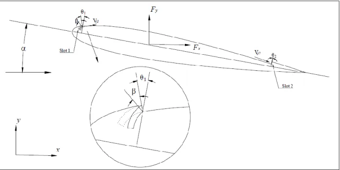
In addition to lift and drag on the airfoil due to free-stream flow, there are additional forces on the airfoil caused by the momentum of the injection jet at the injection slot and suction at the suction slot for the CFJ airfoil. These additional forces are automatically included in the measurement of lift and drag in the wind tunnel. However, in a CFD simulation, ANSYS FLUENT cannot calculate the additional reactionary forces automatically. It can only calculate the forces acting on the surface of airfoil. Therefore, additional reactionary forces are included by using the control volume analysis. For CFJ airfoil without changeable injection angle, Zha et al. [6] give the following formulas Eq. (1) and Eq. (2) for calculating the reactionary forces by using the flow parameters at the injection and suction slots:

𝐹_{𝑥𝑐𝑓𝑗} = (𝑚̇_𝑗𝑉_𝑗1+ 𝑝_𝑗1𝐴_𝑗1) ∗ cos(𝜃₁− 𝛼) − (𝑚̇_𝑗𝑉_𝑗2+ 𝑝_𝑗2𝐴_𝑗2) ∗ cos(𝜃₂ + 𝛼) ₍₁₎

𝐹𝑦𝑐𝑓𝑗 = (𝑚̇𝑗𝑉𝑗1+ 𝑝𝑗1𝐴𝑗1) ∗ sin(𝜃1− 𝛼) + (𝑚̇𝑗𝑉𝑗2+ 𝑝𝑗2𝐴𝑗2) ∗ sin(𝜃2 + 𝛼) ₍₂₎

The subscripts 1 and 2 represent the injection and suction respectively. 𝑚̇_𝑗 is the injection and suction mass flow (injection mass flow is equal to suction mass flow), 𝑉_𝑗 are injection and suction velocities, 𝑝_𝑗 are static pressures at two slots’ exits, 𝐴_𝑗 are areas at two slots’ exits and α

is the angle of attack. 𝜃1 and 𝜃2 respectively are angles between the injection slot and suction

(17)

5

This thesis introduces changeable injection angle 𝛽 into the CFJ airfoil as shown in Figure 3. Based on Figure 3, the formulas to calculate the reactionary forces become:

𝐹_{𝑥𝑐𝑓𝑗} = (𝑚̇_𝑗𝑉_𝑗1+ 𝑝_𝑗1𝐴_𝑗1) ∗ cos(𝜃₁+ 𝛽 − 𝛼) − (𝑚̇_𝑗𝑉_𝑗2+ 𝑝_𝑗2𝐴_𝑗2) ∗ cos(𝜃₂+ 𝛼)₍₃₎

𝐹𝑦𝑐𝑓𝑗 = (𝑚̇𝑗𝑉𝑗1+ 𝑝𝑗1𝐴𝑗1) ∗ sin(𝜃1+ 𝛽 − 𝛼) + (𝑚̇𝑗𝑉𝑗2+ 𝑝𝑗2𝐴𝑗2) ∗ sin(𝜃2+ 𝛼) ₍₄₎

Figure 3: Flow parameters at the injection and suction slots.

The total lift and drag acting on the airfoil then can be expressed as:

𝐷 = 𝑅_𝑥′ − 𝐹_{𝑥𝑐𝑓𝑗} ₍₅₎

𝐿 = 𝑅_𝑦′ _{− 𝐹}

𝑦𝑐𝑓𝑗 ₍₆₎

𝑅_𝑥′ and 𝑅_𝑦′ are the surface integral of pressure and shear stress in the drag and lift direction. Thus, in the numerical simulation, the final drag and lift due to changeable injection angle on NACA0012 airfoil are calculated by the formulas given by Eq. (3), Eq. (4), Eq. (5) and Eq. (6).

(18)

6

2.2 Jet Momentum Coefficient

CFJ airfoil introduces a parameter called jet momentum coefficient 𝐶𝜇 to quantify the

momentum of the injection jet. 𝐶_𝜇 is defined as:

𝐶_𝜇 = 𝑚̇𝑗𝑉𝑗

1

2 𝜌∞𝑉∞2𝑆 (7)

In Eq. (7), 𝑚̇_𝑗 is injection mass flow, 𝑉_𝑗 is the injection velocity, 𝜌_∞ is far field free stream density, 𝑉∞ is the far field free stream velocity and 𝑆 is c, 1 meter. The c is the chord length of

(19)

7

Chapter 3: Physical Model and Mesh

This section describes the flow conditions of the simulation as well as the geometry of the airfoil and structured mesh around it created in ICEM.

3.1 Flow Conditions

The flow past a changeable injection angle CFJ NACA0012 airfoil of chord length 𝑐 = 1.0 𝑚

is investigated. The Mach number is 0.2 and Reynolds number is about 4,564,760. Angle of attack, jet momentum coefficient, injection angle and injection slot location are changed in different cases as shown in Table 1 and Table 2 in section 6.1 and section 6.3 respectively.

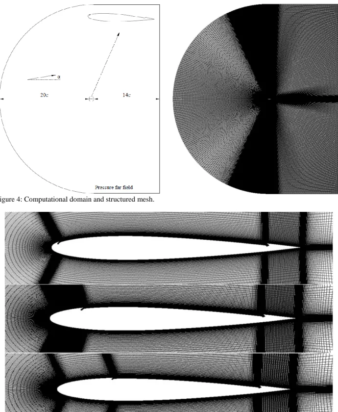
3.2 Geometry and Mesh

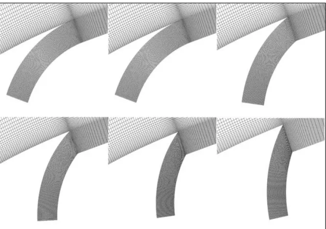
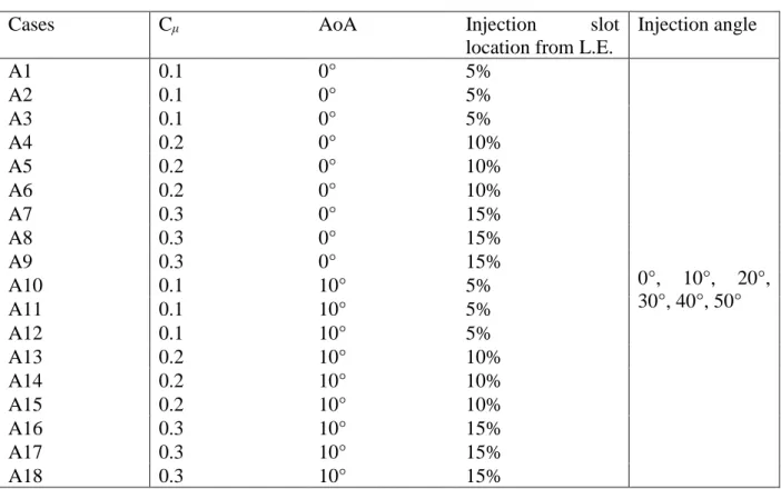
A C-block computational domain is used as shown in Figure 4. The maximum horizontal length of the domain is 35c (20c in front of the airfoil and 14c behind the airfoil) so that the unbounded flow condition can be satisfied during the calculation. Figure 4 also show the structured mesh with refinements near the injection slot and suction slot and in the wake region. The suction slot in all cases is located at 85% chord length but the injection slots are located at 5% chord length, 15% chord length, 25% chord length on the upper surface of the airfoil for different cases as shown in Figure 5. Injection angle changes from 0° to 50° for different cases at each injection slot location as shown in Figure 6. The chord length is 1m, injection slot width is 0.005m and suction slot width is 0.01m. There are 306,750 nodes in the computational domain and the first layer cell height on the airfoil surface is 0.0001m ensuring that y+<1. The external boundary of the computational domain is set as a pressure far field condition.

(20)

8

Figure 4: Computational domain and structured mesh.

(21)

9

Figure 6: Changeable injection angle on the upper surface of the airfoil.

3.3 V

j

with Different Injection Angles

𝑉_𝑗 is a parameter that needs to be specified to calculate 𝐶_𝜇. In the simulation, 𝑉_𝑗 needs to be specified at injection slot exit curve 13 as shown in Figure 7 (a). In ANSYS FLUENT, curve 13 is set as a type of boundary condition called “interior” so that a UDF (user defined function) can extract necessary parameters at curve 13 to calculate 𝑉𝑗. There is no macro command in UDF

that can directly extract velocity at an interior boundary condition. Because UDF has macro command to extract densities at first layer cells on interior boundary’s two sides, average density at curve 13 is known. Thus, injection velocity 𝑉𝑗 can be obtained by the relation:

𝑉_𝑗 = 𝑚̇

(22)

10

where mass flow 𝑚̇ can be extracted at curve 20 (pressure inlet boundary condition) and injection slot exit density 𝜌_𝑗1 can be extracted at curve 13 (interior boundary condition). As Figure 7 (b) shows, 𝐴𝑗1 is the area at injection slot exit (curve 13) and 𝐴𝑗1cos 𝛽 is the vertical

cross section area of the injection slot (curve 17).

𝑉_𝑗 changes with different injection angles 𝛽 even when 𝐶_𝜇 is the same.

Figure 7: Diagrammatic sketch describing how to calculate 𝑉𝑗.

Figure 7 (a) shows the geometry used to create the mesh in ICEM and Figure 7 (b) is a diagrammatic sketch. There is no curve17 in the mesh geometry. Details about the UDF to satisfy a specific 𝐶_𝜇 are given in next section and in Appendix.

(23)

11

Chapter 4: Numerical Method

This section describes the numerical set up employed in ANSYS FLUENT to achieve the simulations of CFJ NACA0012 airfoil using the changeable injection angles.

4.1 ANSYS FLUENT Setup and Boundary Conditions

The double precision solver in ANSYS FLUENT 17.1 is used to perform the CFD simulations. This research employs the 2D Compressible Reynolds-averaged Navier-Stokes equations with Spalart-Allmaras turbulence model. A Second-order numerical scheme is used for discretization of both the convection and diffusion terms. The pressure-coupled transient solver is used for pseudo-transient pressure-velocity coupling. Steady solver is employed in the simulations with pseudo-transient method. When results show a steady flow, convergence is considered achieved if lift coefficient and drag coefficient change within 0.01% over 1000 iterations. When results show an unsteady flow, convergence is considered achieved if lift coefficient and drag coefficient become periodic after several cycles and do not change from one cycle to next cycle; 20 cycles are chosen as the time average period to calculate the average aerodynamic coefficients for the unsteady periodic flow.

No slip wall condition is used on the airfoil solid surface and on the injection and suction slot two side walls. Pressure-far-field condition with Mach number = 0.2 and total pressure = 0 are set to satisfy the far-field unbounded flow boundary conditions at the outer boundary of the computational domain. The inlet of injection slot is set as pressure inlet condition with changeable total pressure controlled by UDF. The exit of suction slot is set as a pressure outlet condition with changeable static pressure controlled by UDF. The operating condition is one standard atmospheric pressure.

(24)

12

4.2 UDF of C

μ

Iteration

CFJ airfoil must achieve zero net mass flux under all operating conditions. The mass flow exiting from injection slot 𝑚̇_𝑖𝑛𝑗 must be equal to the mass flow entering the suction slot 𝑚̇_𝑠𝑢𝑐. The momentum of the flow is defined by 𝐶𝜇 and a specific value of 𝐶𝜇 is achieved by adjusting

the injection slot inlet total pressure 𝑃_𝑡_𝑖𝑛𝑗. The 𝑚̇_𝑠𝑢𝑐 matches 𝑚̇_𝑖𝑛𝑗 by adjusting the suction slot exit static pressure 𝑃_𝑠_𝑠𝑢𝑐. During each iteration, there is a UDF process to judge whether the above two conditions are achieved by adjusting the 𝑃_𝑡_𝑖𝑛𝑗 and 𝑃_𝑠_𝑠𝑢𝑐 automatically. The acceptable variation for 𝐶_𝜇 and mass flow are both within 0.2% for this research.

(25)

13

Chapter 5: Validation of Numerical Method

The numerical investigation of the flow field of NACA0012 airfoil at Reynolds number of

𝑅𝑒 = 6 × 106_{at angle of attack is}_10°_{and chord length is 1 meter is conducted to validate the}

numerical method in ANSYS FLUENT. The pressure coefficient 𝐶_𝑝 is plotted against x/c in Figure 8. The experimental results are from Gregory and O’Reilly [19].

Figure 8: Pressure coefficient for flows past NACA0012 airfoil; 𝑅𝑒 = 6 × 106_,_{𝛼 = 10°}_.

-2 -1 0 1 2 3 4 5 6 7 -0.2 0 0.2 0.4 0.6 0.8 1 1.2 Cp x/c NACA0012

Upper airfoil surface Lower airfoil surface Gregory's data

(26)

14

The numerical results using the compressible RANS equations agree quite well with the experimental data as shown in Figure 8. The streamlines and velocity vectors are shown in Figure 9.

(27)

15

Chapter 6: Results and Discussion

6.1 Changeable injection angle’s influence on aerodynamic

coefficients

As shown in Table 1, 18 different cases were computed and compared to study the influence of changeable injection angle on the aerodynamic coefficients with different 𝐶_𝜇, angle of attack and injection slot location. From these results, a best injection location can be determined by exercising control using the changeable injection angle CFJ.

Cases Cμ AoA Injection slot

location from L.E.

Injection angle A1 0.1 0° 5% 0°, 10°, 20°, 30°, 40°, 50° A2 0.1 0° 5% A3 0.1 0° 5% A4 0.2 0° 10% A5 0.2 0° 10% A6 0.2 0° 10% A7 0.3 0° 15% A8 0.3 0° 15% A9 0.3 0° 15% A10 0.1 10° 5% A11 0.1 10° 5% A12 0.1 10° 5% A13 0.2 10° 10% A14 0.2 10° 10% A15 0.2 10° 10% A16 0.3 10° 15% A17 0.3 10° 15% A18 0.3 10° 15%

Table 1: Geometry parameters for CFJ airfoil with changeable injection angle.

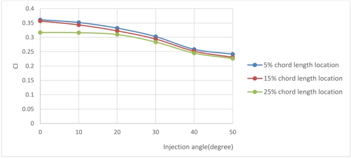
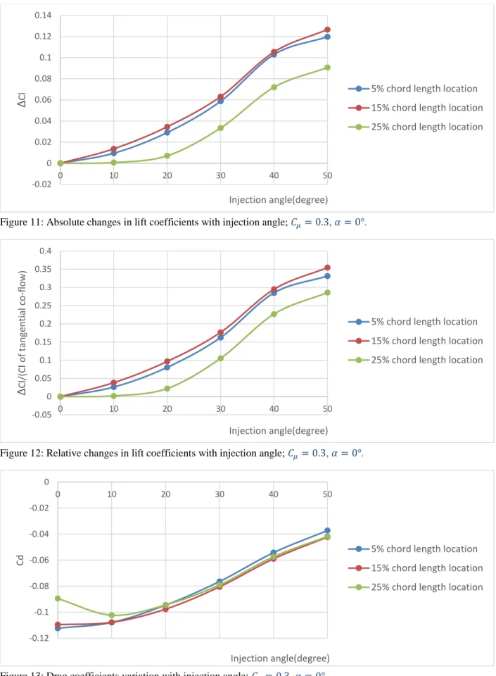
Figures 10-13 show the results for cases A7, A8, A9 and Figure 14-17 show the results for cases A16, A17, A18. These figures show the change in aerodynamic coefficients with different injection angles when injection locations are different. Cases A7, A8, A9 and A16, A17, A18 are all computed for 𝐶_𝜇 = 0.3.

(28)

16

Figure 10 shows the variation in lift coefficient with injection angle for 𝐶_𝜇 = 0.3 and angle of attack = 0°. It shows that 5% and 15% chord length location of injection slot have nearly same lift coefficient with change in injection angle and their lift coefficients are all higher than these obtained for 25% chord length location of injection angle. Also, as injection angle becomes larger, the lift coefficient becomes smaller as expected. Figure 11 and Figure 12 show the absolute change and the relative change in lift coefficients at different injection angles compared to their respective tangential flow case. Figure 11 and Figure 12 show that when injection location is located at 15% chord length, the change in injection angle can produce most significant decrease in lift. The maximum decrease in lift can be 35% compared to its corresponding tangential flow case with absolute lift coefficient decreasing by 0.122.

Figure 13 shows that the drag coefficient increases when injection angle becomes larger. Also, the injection slot at 15% chord length location has the smallest drag coefficient.

Figure 10: Lift coefficients variation with injection angle; 𝐶𝜇= 0.3, 𝛼 = 0°.

0 0.05 0.1 0.15 0.2 0.25 0.3 0.35 0.4 0 10 20 30 40 50 Cl Injection angle(degree)

5% chord length location 15% chord length location 25% chord length location

(29)

17

Figure 11: Absolute changes in lift coefficients with injection angle; 𝐶𝜇= 0.3, 𝛼 = 0°.

Figure 12: Relative changes in lift coefficients with injection angle; 𝐶𝜇= 0.3, 𝛼 = 0°.

Figure 13: Drag coefficients variation with injection angle; 𝐶𝜇= 0.3, 𝛼 = 0°.

-0.02 0 0.02 0.04 0.06 0.08 0.1 0.12 0.14 0 10 20 30 40 50 Δ Cl Injection angle(degree)

-0.05 0 0.05 0.1 0.15 0.2 0.25 0.3 0.35 0.4 0 10 20 30 40 50 Δ Cl /(C l o f t an ge n tia l co -f low) Injection angle(degree)

-0.12 -0.1 -0.08 -0.06 -0.04 -0.02 0 0 10 20 30 40 50 Cd Injection angle(degree)

(30)

18

Figures 14-17 show the results of computation when 𝛼 = 0° and 𝐶_𝜇 = 0.3. Figures 14-16 show that when injection slot is at 5% and 15% chord length location, the lift coefficients have nearly the same values and are all higher than that value at 25% chord length location of the injection slot. The decrease in maximum absolute lift coefficient is 0.2 and the decrease in maximum relative lift coefficient is 0.12. Thus, when the angle of attack becomes larger, the influence of change in injection angle on lift coefficient becomes relatively smaller.

Figure 17 shows that when injection slot is at 15% chord length location, the drag coefficient has minimum value. But as the injection angle becomes larger, drag coefficient increases.

1.4 1.45 1.5 1.55 1.6 1.65 0 10 20 30 40 50 Cl Injection angle(degree)

0 0.05 0.1 0.15 0.2 0.25 0 10 20 30 40 50 Δ Cl Injection angle(degree)

(31)

19

Figure 16: Relative changes in lift coefficients with injection angle; 𝐶𝜇= 0.3 , 𝛼 = 10° .

Figures 18-21 show the results for A4, A5, A6 cases and the Figure 22-25 show the results for A13, A14, A15 cases. Cases A4, A5, A6 and A13, A14, A15 cases are computed with 𝐶_𝜇 = 0.2.

Figure 18 shows when 𝐶𝜇 = 0.2 and α = 0°, the influence of changeable injection angle on lift

coefficient is nearly the same at different injection locations. Since 𝐶_𝜇 becomes smaller, all lift coefficients with different injection angles become smaller. From Figure 19 and Figure 20, changes in absolute lift coefficients and the relative lift coefficients also become smaller. When

0 0.02 0.04 0.06 0.08 0.1 0.12 0.14 0 10 20 30 40 50 Δ Cl /(C l o f t an ge n tia l co -f low) Injection angle(degree)

(32)

20

𝐶_𝜇 = 0.2 and α = 0°, 15% and 25% chord length locations of injection slot have higher changes

in relative lift coefficients compared to 5% chord length location. At 15% chord length location of the injection slot, the maximum change in lift coefficient is about 25% and at 25% chord length location, the maximum change in lift coefficient is about 27%.

Figure 21 shows that at 5% and 15% chord length locations of injection slot, the drag coefficients become smaller than that at 25% chord length location of the injection slot and as the injection angle becomes larger, drag coefficient becomes larger.

0 0.05 0.1 0.15 0.2 0.25 0.3 0 10 20 30 40 50 Cl Injection angle(degree)

0 0.01 0.02 0.03 0.04 0.05 0.06 0.07 0.08 0 10 20 30 40 50 Δ Cl Injection angle(degree)

(33)

21

Figures 22-24 show the lift coefficients, absolute changes in lift coefficients and relative changes in lift coefficients when 𝐶𝜇 = 0.2 and α =10°. At 15% chord length location of injection

slot, the lift coefficients with different injection angle are larger than that for the 5% and 25% chord length location but the 15% chord length location has smaller relative changes in lift coefficients. When angle of attack becomes larger, the relative changes in lift coefficients

0 0.05 0.1 0.15 0.2 0.25 0.3 0 10 20 30 40 50 Δ Cl /(C l o f t an ge n tia l co -f low) Injection angle(degree)

-0.07 -0.06 -0.05 -0.04 -0.03 -0.02 -0.01 0 0 10 20 30 40 50 Cd Injection angle(degree)

(34)

22

become smaller. When 𝐶_𝜇 = 0.2 and α = 10°, the maximum relative changes in lift coefficient at 5% chord length location of the injection slot is 5.5% and at 15% chord length location of the injection slot is 4.5%.

Figure 25 shows that the drag coefficients are smallest at 15% chord length location for different injection slot locations.

1.36 1.37 1.38 1.39 1.4 1.41 1.42 1.43 1.44 1.45 1.46 0 10 20 30 40 50 Cl Injection angle(degree)

0 0.01 0.02 0.03 0.04 0.05 0.06 0.07 0.08 0.09 0 10 20 30 40 50 Δ Cl Injection angle(degree)

(35)

23

Figures 26-29 show the results for A1, A2, A3 cases and Figures 30-33 show the results for A10, A11, A12 cases. Cases A1, A2, A3 and A10, A11, A12 are computed with 𝐶_𝜇 = 0.1.

Figure 18 shows that when 𝐶𝜇 = 0.1 and α = 0°, the influence of changeable injection angle

on lift coefficients is nearly the same at different locations of the injection slot. From Figures 27-28, the maximum absolute changes and relative changes in lift coefficient are at 15% and 25%

(36)

24

chord length location of the injection slot. Both the two locations have almost the same maximum relative change in lift coefficient which is about 25%.

Figure 29 shows that at 15% chord length location, the drag coefficients are always minimum among the three different locations of the injection slot with different injection angles when 𝐶_𝜇 = 0.1 and α = 0°.

0 0.02 0.04 0.06 0.08 0.1 0.12 0.14 0.16 0.18 0 10 20 30 40 50 Cl Injection angle(degree)

0 0.005 0.01 0.015 0.02 0.025 0.03 0.035 0.04 0.045 0 10 20 30 40 50 Δ Cl Injection angle(degree)

(37)

25

Figures 30-33 show the results of aerodynamic coefficients that when 𝐶_𝜇 = 0.1 and α = 10°. When the injection angle becomes 50°, there are some sharp changes in aerodynamic coefficients with injection slot at 5% chord length location. The sharp changes are not desirable for changeable injection angle control. These sharp changes are described in next section.

-0.025 -0.02 -0.015 -0.01 -0.005 0 0 10 20 30 40 50 Cd Injection angle(degree)

(38)

26

From Figure 30, when the injection slot is located at 15% and 25% chord length location, lift coefficients have higher value compared to when the injection slot located at 5% chord length location. From Figure 31-32, the change in maximum absolute lift coefficient is about 0.06 and the change in maximum relative lift coefficient is about 5% (ignoring the sharp change at very high injection angle).

Figure 33 shows that when 𝐶_𝜇 = 0.1 and α = 10°, 15% chord length location has minimum drag coefficient among the three different injection slot locations.

1.18 1.2 1.22 1.24 1.26 1.28 1.3 1.32 1.34 1.36 0 10 20 30 40 50 Cl Injection angle(degree)

(39)

27

0 0.02 0.04 0.06 0.08 0.1 0.12 0.14 0 10 20 30 40 50 Δ Cl Injection angle(degree)

0 0.01 0.02 0.03 0.04 0.05 0.06 0.07 0.08 0.09 0.1 0 10 20 30 40 50 Δ Cl /(C l o f t an ge n tia l co -f low) Injection angle(degree)

-0.02 -0.015 -0.01 -0.005 0 0.005 0.01 0.015 0.02 0 10 20 30 40 50 Cd Injection angle(degree)

(40)

28

6.2 Sharp change in aerodynamic coefficient for a

combination of

𝑪

_𝝁

, injection slot location and high injection

angle

From section 6.1, it can be noted that there is a sharp change in aerodynamic coefficients when injection slot is located at 5% chord length location, 𝐶𝜇 = 0.1, α = 10° and injection angle is 50°.

However, when injection slot is located at 15% or 25% chord length location, there is no sharp change in aerodynamic coefficients. To explain this phenomenon more clearly, the influence of injection angle from 0° to 60° is studied for various locations of the injection slot when 𝐶𝜇 = 0.1.

The results are shown in Figure 34 and 35. When the injection angle becomes 60°, there is sharp change in Cl and Cd when injection slot is at 5% chord length location and there is no sharp change when injection slot is located at 15% or 25% injection location.

0 0.2 0.4 0.6 0.8 1 1.2 1.4 1.6 0 10 20 30 40 50 60 Cl Injection angle(degree)

(41)

29

Figure 36 shows the streamlines and velocity vectors around the NACA0012 airfoil in different injection angles when 𝐶𝜇 = 0.1, α = 10° and injection slot is at 5% chord length

location. Figure 37 shows the streamlines and vectors around the NACA0012 airfoil at different injection angles when 𝐶_𝜇 = 0.1, α =10° and injection slot is at 15% chord length location. It shows that when injection slot is located at 5% chord length location, the flow separation occurs when injection angle is 60°.

Figures 38-40 show the streamlines and velocity vectors near the injection slots when injection angles are all 60°. It shows that when injection slot is at 15% or 25% chord length location, there is no obvious flow separation like the one observed when injection slot is at 5% chord length location. -0.04 -0.02 0 0.02 0.04 0.06 0.08 0.1 0.12 0.14 0 10 20 30 40 50 60 Cd Injection angle(degree)

(42)

30

injection angle = 10° injection angle = 20°

Figure 36: Streamlines and velocity vectors for 10° to 60° injection angles at 5% chord length location when 𝐶𝜇=

(43)

31

Figure 37: Streamlines and velocity vectors for 10° to 60° injection angles at 15% chord length location when 𝐶𝜇=

(44)

32

Figure 38: Streamlines and velocity vectors for 60° injection angles at 5% chord length location when 𝐶𝜇= 0.1 and

𝛼 = 10°.

Figure 39: Streamlines and velocity vectors for 60° injection angles at 15% chord length location when 𝐶𝜇= 0.1

(45)

33

Figure 40: Streamlines and velocity vectors for 60° injection angles at 25% chord length location when 𝐶𝜇= 0.1

and 𝛼 = 10°.

To define a best injection slot location to increase the stall margin, there are different aspects that need to be considered. First, when injection slot location is at 5% chord length location, it has relatively smaller injection angle range without the sharp change in Cl and Cd, 0° to 40°. When injection slot location is at 15% or 25%, the injection angle range is at least from 0° to 60° without sudden change in Cl and Cd. Second, from the results in section 6.1, when injection slot location is at 5% or 15% chord length location, the NACA0012 airfoil has relatively larger changes in absolute lift coefficient and in the relative lift coefficient compared to when injection slot location is at 25% chord length location. When injection slot location is at 5% or 15% chord length location and 𝐶𝜇 = 0.3, the NACA0012 airfoil has relatively larger lift coefficients at all

different injection angles compared to when injection slot location is at 25% chord length location and 𝐶_𝜇 = 0.3. When injection slot location is at 15% chord length location and 𝐶_𝜇 = 0.2

(46)

34

or 0.1, the NACA0012 airfoil has the largest lift coefficients for most injection angles. Third, for most of the cases in Table 1, when injection slot location is at 15% chord length, the drag coefficients are the smallest.

Thus, after considering sharp changes in Cl and Cd in both the relative and absolute lift coefficients for large injection angles, 15% chord length location appears to be the best injection slot location for changeable injection angles technology for CFJ.

6.3 Injection angle’s influence on stall angle

As shown in Table 2, nine different cases are studied to find the influence of injection angle on stall angle. Because the largest injection angle that does not cause sharp change when injection slot is at 5% chord length is 40°. 40° is chosen in B5 to B8 to study the influence on stall angle of the injection angle. In this section, flow pass CFJ NACA0012 airfoil with changeable injection angle is compared to the flow past a traditional tangential CFJ NACA0012 airfoil. From results in section 6.1 and section 6.2, when the injection slot is at 25% chord length location, the airfoil has worst results for aerodynamic coefficients, thus 25% chord length location is not studied in this section.

Cases Cμ Injection angle Injection slot location AoA

B1 0.1 0° 5% Around the stall angle B2 0.2 0° 5% B3 0.1 0° 15% B4 0.2 0° 15% B5 0.1 40° 5% B6 0.2 40° 5% B7 0.1 40° 15% B8 0.2 40° 15%

B9(original airfoil) N/A N/A N/A

(47)

35

Figure 41 shows the results of cases B1, B2 and B9 and Figure 42 shows the results of cases B5, B6 and B9. Figures 41 and 42 show the aerodynamic coefficients for different angle of attack when injection slot is at 5% chord length location.

From Zha et al.’s papers [5-7], it can be noted for a thick airfoil like NACA0025, the tangential CFJ control can increase the stall angle significantly. However, NACA0012 airfoil is a thin airfoil and thus the increase in stall angle of tangential CFJ control is not significant. Figure 41 shows that the original NACA0012 airfoil has stall angle of 17° and tangential CFJ NACA0012 airfoil has stall angle at 20° when 𝐶_𝜇 is 0.1 or 0.2.

Figure 42 shows the results when the injection angle becomes 40°. This figure shows that, when the injection slot is at 5% chord length location, there is a significant decrease in stall angle if injection angle becomes larger. When 𝐶_𝜇 is 0.1 and injection angle is 40°, the stall angle becomes 14°. When 𝐶_𝜇 is 0.2 and injection angle is 40°, the stall angle becomes 17°.

(48)

36

Figure 41: Stall angle analysis when injection slot is at 5% chord length location and injection angle is 0°.

0 0.5 1 1.5 2 2.5 0 5 10 15 20 25 30 Cl AOA

Cl when injection slot is at 5% chord length location and

injection angle is 0

°

Cl vs AOA of NACA0012 Cl vs AOA of Cmu=0.1 Cl vs AOA of Cmu=0.2 -0.1 0 0.1 0.2 0.3 0.4 0.5 0.6 0 5 10 15 20 25 30 Cd AOA

Cd when injection slot is at 5% chord length location and

injection angle is 0

°

Cd vs AOA of NACA0012 Cd vs AOA of Cmu=0.1 Cd vs AOA of Cmu=0.2

(49)

37

Figure 43 shows the results of B3, B4 and B9 and Figure 44 shows the results of B7, B8 and B9. Figures 43 and 44 show the aerodynamic coefficients at different angle of attack when injection slot is at 15% chord length location.

0 0.5 1 1.5 2 2.5 0 5 10 15 20 25 30 Cl AOA

Cl when injection slot is at 5% chord length location and

injection angle is 40

°

Cl vs AOA of NACA0012 Cl vs AOA of Cmu=0.1 Cl vs AOA of Cmu=0.2 -0.05 0 0.05 0.1 0.15 0.2 0.25 0.3 0.35 0 5 10 15 20 25 30 Cd AOA

Cd when injection slot is at 5% chord length location and

injection angle is 40

°

(50)

38

Figure 43 shows that the increase in stall angle caused by tangential CFJ NACA0012 airfoil is still small when injection slot is at 15% chord length location. When 𝐶𝜇 = 0.1, the stall angle is

19° and when 𝐶𝜇 = 0.2, the stall angle is 18°. Figure 44 shows the results when injection angle

becomes 40° and injection slot is at 15% chord length location. It shows that the stall angle is 20° when 𝐶𝜇 = 0.1 and stall angle is 18° when 𝐶𝜇=0.2. Thus, when injection slot is at 15% chord

length location, the change in stall angle caused by changeable injection angle is very small.

0 0.5 1 1.5 2 2.5 0 5 10 15 20 25 30 Cl AOA

Cl when injection slot is at 15% chord length location and

injection angle is 0

°

Cl vs AOA of NACA0012 Cl vs AOA of Cmu=0.1 Cl vs AOA of Cmu=0.2 -0.1 -0.05 0 0.05 0.1 0.15 0.2 0.25 0.3 0.35 0 5 10 15 20 25 30 Cd AOA

Cd when injection slot is at 15% chord length location and

injection angle is 0

°

(51)

39

It can be concluded that, when injection angle is changed from 0° to 40°, if injection slot is at 5% chord length location, there will be a significant decrease in stall angle and the stall angle will become smaller than the stall angle of original NACA0012 airfoil. When injection angle is changed from 0° to 40°, if injection slot is at 15% chord length location, there will be very small

0 0.5 1 1.5 2 2.5 0 5 10 15 20 25 30 Cl AOA

Cl when injection slot is at 15% chord length location and

injection angle is 40

°

Cl vs AOA of NACA0012 Cl vs AOA of Cmu=0.1 Cl vs AOA of Cmu=0.2 -0.1 -0.05 0 0.05 0.1 0.15 0.2 0.25 0.3 0.35 0 5 10 15 20 25 30 Cd AOA

Cd when injection slot is at 15% chord length location and

injection angle is 40

°

(52)

40

change in the stall angle and the stall angle is nearly the same as the stall angle of original NACA0012 airfoil.

Thus, 15% chord length location is the best location for injection slot to implement the changeable injection angle technology with CFJ for controlling the lift and drag of an airfoil.

(53)

41

Chapter 7: Conclusions

This thesis has studied the influence on aerodynamic coefficients of NACA0012 airfoil when changeable injection angle CFJ control technology is employed to modulate its lift and drag coefficient. By comparing the aerodynamic performance of changeable injection angle CFJ control method with tangential CFJ control method, a best injection slot location is found from the three different locations considered that can employ the changeable injection angle CFJ technology to change the aerodynamic coefficients significantly but having little influence on stall angle. The main conclusions can be summarized as the follows:

1) Changeable injection angle CFJ technology can be employed to control the aerodynamic coefficients of an airfoil. When the injection angle becomes larger, the lift coefficient becomes smaller and drag coefficient becomes larger.

2) Changeable injection angle CFJ control method has influence on stall angle of an airfoil. When injection angle becomes larger, the stall angle becomes smaller.

3) For different injection slot locations, the influence of changeable injection angle CFJ control method on aerodynamic coefficients and stall angle is very different. After comparing the aerodynamic coefficients at three different locations of injection slot on the airfoil with various 𝐶𝜇 = 0.1, 0.2 and 0.3, and AoA of 0° and 10°, it was found that when

injection slot is at 15% chord length location, the NACA0012 airfoil always has relatively larger lift coefficient and smaller drag coefficient and has larger relative changes in lift coefficients for most of the cases.

4) When 𝐶_𝜇 becomes larger and AoA becomes smaller, the relative changes in lift coefficients become larger for all injection angles. When 𝐶𝜇 is 0.3 and AoA is 0° and

(54)

42

injection slot is at 15% chord length location (Figure 12), changeable injection angle CFJ technology has largest relative changes in lift coefficients for all injection angles. When injection angle becomes 50°, the relative change in lift coefficient can be 35%.

5) When injection slot location is at 5% chord length location, there is a sharp change in aerodynamic coefficients when injection angle becomes 40°. When injection slot location is at 15% or 25% chord length location, there is no sharp change in aerodynamic coefficients when injection angle changes from 0 °to 60°.

6) When injection slot is at 5% chord length location, there is significant decrease in stall angle when injection angle changes from 0° to 40°. When injection slot is at 15% chord length location, there is nearly no change in stall angle when injection angle changes from 0° to 40°.

Thus, it can be concluded that the changeable injection angle CFJ technology can control the aerodynamic coefficients and the best injection slot location to employ this technology is at 15% chord length location for NACA0012 airfoil. The changeable injection angle method can be effectively used by appropriately changing the 𝐶𝜇 to control the aerodynamic coefficients of the

(55)

43

References

[1]. Lefebvre, A. and Zha, G.-C., “Design of High Wing Loading Compact Electric Airplane Utilizing Co-Flow Jet Flow Control,” AIAA Paper 2015-0772, AIAA SciTech2015: 53nd Aerospace Sciences Meeting, Kissimmee, FL, 5-9 Jan 2015.

[2]. Zha, G.-C., Paxton, C., Conley, A., Wells, A., and Carroll, B., “Effect of Injection Slot Size on High Performance Co-Flow Jet Airfoil,” Journal of Aircraft, Vol. 43, No. 4, July-Aug. 2006, pp. 987–995.

[3]. Dano, B. P. E., Kirk, D., and Zha, G.-C., “Experimental Investigation of Jet Mixing Mechanism of Co- Flow Jet Airfoil,” AIAA Paper 2010-4421, 5th AIAA Flow Control Conference, Chicago, IL, 28 Jun - 1 Jul 2010.

[4]. Dano, B. P. E., Zha,G.-C., and Castillo, M., “Experimental Study of Co-Flow Jet Airfoil Performance Enhancement Using Micro Discreet Jets,” AIAA Paper 2011-0941, 49th AIAA Aerospace Sciences Meeting, Orlando, FL, 4-7 January 2011.

[5]. Zha, G.-C., Carroll, B., Paxton, C., Conley, A., and Wells, A., “High Performance Airfoil with Co-Flow Jet Flow Control,” AIAA Paper 2005-1260, 43rd AIAA Aerospace Sciences Meeting, Reno, NV, 10-13 January 2005.

[6]. Zha, G.-C., Gao, W., and Paxton, D. C., “Jet Effects on Co-flow Jet Airfoil Performance,” AIAA Journal, Vol. 45, No. 6, 2007, pp. 1222-1231.

[7]. Zha, G.-C., and Paxton, D. C., “A Novel Flow Control Method for Airfoil Performance Enhancement Using Co-Flow Jet,” Progress in Astronautics and Aeronautics, Chapter10 - Applications of Circulation Control Technologies, Editors: Joslin, R. D. and Jones, G.S., Vol. 214, AIAA, Reston, VA, 2006, pp. 293-314.

[8]. Wang, B.-Y. and Haddoukessouni, B. and Levy, J. and Zha, G.-C., “Numerical Investigations of Injection Slot Size Effect on the Performance of Co-Flow Jet Airfoil," Journal of Aircraft, Vol. 45, No. 6, 2008, pp.2084-2091.

[9]. Lefebvre, A. and Dano, B. and Bartow, W. and Di Franzo, M. and Zha, G.-C., “Performance Enhancement and Energy Expenditure of Co-Flow Jet Airfoil with Variation of Mach number,” AIAA Paper 2013-0490, AIAA Journal of Aircraft, DOI: 10.2514/1.C033113, 2016.

[10]. Yang, Y., and Zha, G.-C., “Super-Lift Coefficient of Active Flow Control Airfoil: What is the Limit?” AIAA Paper 2017-1693, AIAA SciTech 2017, 55th AIAA Aerospace Science Meeting, Grapevine, TX, 9-13 January 2017.

[11]. Liu, Z.-X., and Zha, G.-C., “Transonic Airfoil Performance Enhancement Using Co-Flow Jet Active Flow Control,” AIAA Paper 2016-3066, AIAA Aviation, 13 -17 June 2016.

(56)

44

[12]. Anders, S., Sellers, W. L., and Washburn, A., “Active Flow Control Activities at NASA

Langley,” AIAA Paper 2004-2623, June 2004.

[13]. Miller, D., and Addington, G., “Aerodynamic Flowfield Control Technologies for Highly

Integrated Airframe Propulsion Flowpaths,” AIAA Paper 2004-2625, June 2004.

[14]. Sellers, W. L. I., Singer, B. A., and Leavitt, L. D., “Aerodynamics for Revolutionary Air

Vehicles,” AIAA Paper 2004-3785, June 2003.

[15]. Kibens, V., and Bower, W. W., “An Overview of Active Flow Control Applications at

the Boeing Company,” AIAA Paper 2004-2624, June 2004.

[16]. Tilmann, C. P., Kimmel, R. L., Addington, G., and Myatt, J. H., “Flow Control Research

and Application at the AFRL’s Air Vehicles Directorate,” AIAA Paper 2004-2622, June 2004.

[17]. Gad-el Hak, M., Flow Control, Passive, Active, and Reactive Flow Management, Cambridge Univ. Press, Cambridge, England, 2000.

[18]. Gad-el Hak, M., “Flow Control: The Future,” Journal of Aircraft, Vol. 38, No. 3, 2001, pp. 402–418.

[19]. Gregory, Nigel, and C. L. O'reilly, “Low-Speed Aerodynamic Characteristics of NACA 0012 Airfoil Section Including the Effects of Upper-Surface Roughness Simulating Hoar Frost,” HM Stationery Office, London, 1973.

(57)

45

Appendix

UDF for C

μ

#include "udf.h" #include "math.h" #define FARLET_INDEX 82 #define INLET_INDEX 13 #define OUTLET_INDEX 14 #define INTERFACE_INDEX 38 #define S 1 #define injectionsize 0.005 #define tarvalue_Cmu 0.1

static float flow_inlet; static float flow_outlet; static float pressure_inlet_0; static float pressure_inlet_1; static float pre_pressure_inlet_1; static float change_pressure_inlet_1; static float pressure_outlet_0; static float pressure_outlet_1; static float calvalue_Cmu; static float pre_Cmu; static float change_Cmu; static float pre_flow_outlet; static float change_flow_outlet;

(58)

46 Domain *domain; Thread *thread_inlet; Thread *thread_outlet; Thread *thread_farlet; Thread *thread_interface;

void calculate_Cmu(Thread *thread_farlet, Thread *thread_outlet, Thread *thread_inlet, Thread *thread_interface)

{

/* velocity from interface, divided by density and injectionsize, with cell loop, both density and pressure based, for parallel*/

cell_t c; cell_t c0; cell_t c1; face_t f; Thread *t0; Thread *t1; int i = 0; float velocity[2]; float velocity_farlet = 0.0; float velocity_inlet = 0.0; float local_velocity_inlet = 0.0; float density_farlet = 0.0; float density_inlet = 0.0; float density_interface = 0.0; flow_inlet = 0.0; flow_outlet = 0.0; pressure_inlet_0 = 0.0; pressure_outlet_0 = 0.0;

(59)

47 #if !RP_HOST begin_f_loop(f, thread_farlet) { if (PRINCIPAL_FACE_P(f,thread_farlet)) { c0 = F_C0(f, thread_farlet); t0 = F_C0_THREAD(f, thread_farlet); density_farlet += C_R(c0, t0); velocity[0] = C_U(c0, t0); velocity[1] = C_V(c0, t0); velocity_farlet += NV_MAG(velocity); i++; } } end_f_loop(f, thread_farlet) # if RP_NODE density_farlet = PRF_GRSUM1(density_farlet); velocity_farlet = PRF_GRSUM1(velocity_farlet); i = PRF_GRSUM1(i); # endif #endif node_to_host_float_2(density_farlet, velocity_farlet); node_to_host_int_1(i); #if !RP_NODE

(60)

48

density_farlet = density_farlet/i; velocity_farlet = velocity_farlet/i;

Message("moniter density_farlet = %f\n", density_farlet); #endif #if !RP_HOST i = 0; begin_f_loop(f, thread_outlet) { if (PRINCIPAL_FACE_P(f,thread_outlet)) {

flow_outlet += F_FLUX(f, thread_outlet); pressure_outlet_0 += F_P(f, thread_outlet); i++; } } end_f_loop(f, thread_outlet) # if RP_NODE flow_outlet = PRF_GRSUM1(flow_outlet); pressure_outlet_0 = PRF_GRSUM1(pressure_outlet_0); i = PRF_GRSUM1(i); # endif #endif node_to_host_float_2(flow_outlet, pressure_outlet_0); node_to_host_int_1(i);

(61)

49 #if !RP_NODE pressure_outlet_0 = pressure_outlet_0/i; #endif #if !RP_HOST i = 0; begin_f_loop(f, thread_inlet) { if (PRINCIPAL_FACE_P(f,thread_inlet)) {

flow_inlet += F_FLUX(f, thread_inlet); pressure_inlet_0 += F_P(f, thread_inlet); i++; } } end_f_loop(f, thread_inlet) # if RP_NODE flow_inlet = PRF_GRSUM1(flow_inlet); pressure_inlet_0 = PRF_GRSUM1(pressure_inlet_0); i = PRF_GRSUM1(i); # endif #endif node_to_host_float_2(flow_inlet, pressure_inlet_0); node_to_host_int_1(i);

(62)

50 #if !RP_NODE pressure_inlet_0 = pressure_inlet_0/i; #endif #if !RP_HOST i = 0; begin_f_loop(f, thread_inlet) { if (PRINCIPAL_FACE_P(f,thread_inlet)) { c0 = F_C0(f, thread_inlet); t0 = F_C0_THREAD(f, thread_inlet); density_inlet += C_R(c0, t0); i++; } } end_f_loop(f, thread_inlet) # if RP_NODE density_inlet = PRF_GRSUM1(density_inlet); i = PRF_GRSUM1(i); # endif #endif node_to_host_float_1(density_inlet); node_to_host_int_1(i);

(63)

51

#if !RP_NODE

density_inlet = density_inlet/i;

Message("moniter density_inlet = %f\n", density_inlet); local_velocity_inlet = flow_inlet/density_inlet/injectionsize; #endif #if !RP_HOST i = 0; begin_f_loop(f, thread_interface) { if (PRINCIPAL_FACE_P(f,thread_interface)) { c0 = F_C0(f, thread_interface); c1 = F_C1(f, thread_interface); t0 = F_C0_THREAD(f, thread_interface); t1 = F_C1_THREAD(f, thread_interface); density_interface += (C_R(c0, t0)+C_R(c1, t1))/2.0; i++; } } end_f_loop(f, thread_interface) # if RP_NODE density_interface = PRF_GRSUM1(density_interface); i = PRF_GRSUM1(i);

(64)

52 # endif #endif node_to_host_float_1(density_interface); node_to_host_int_1(i); #if !RP_NODE density_interface = density_interface/i;

Message("moniter density_interface = %f\n", density_interface); velocity_inlet = flow_inlet/density_interface/injectionsize;

velocity_inlet = fabs(velocity_inlet);

Message("moniter velocity_inlet(interface) = %f\n", velocity_inlet);

if(density_inlet* velocity_inlet != 0.0) {

pressure_inlet_0 = pressure_inlet_0+ 1/ 2.0* density_inlet*

local_velocity_inlet* local_velocity_inlet; }

Message("moniter pressure_inlet = %f\n", pressure_inlet_0); Message("moniter pressure_outlet = %f\n", pressure_outlet_0);

if(density_farlet* velocity_farlet != 0.0) {

calvalue_Cmu = flow_inlet* velocity_inlet/ (1/ 2.0* density_farlet* velocity_farlet* velocity_farlet* S);

}

calvalue_Cmu = fabs(calvalue_Cmu); change_Cmu = calvalue_Cmu-pre_Cmu;

(65)

53 pre_Cmu = calvalue_Cmu; change_flow_outlet = flow_outlet-pre_flow_outlet; pre_flow_outlet = flow_outlet; #endif } DEFINE_INIT(Initialze_variable,domin) { /*349265*/ calvalue_Cmu = tarvalue_Cmu; pre_pressure_inlet_1 = 0; change_pressure_inlet_1 = 0; pre_Cmu = 0; change_Cmu = 0; pre_flow_outlet = 0; change_flow_outlet = 0; pressure_inlet_1 = 100000; pressure_outlet_1 = -10000; #if !RP_NODE Message("calvalue_Cmu = %f\t", calvalue_Cmu); Message("flow_inlet = %f\t", flow_inlet); Message("flow_outlet = %f\n", flow_outlet); #endif } DEFINE_EXECUTE_AT_END(Set_EachIterate_masstwopercentchange) { domain = Get_Domain(1);

(66)

54

thread_inlet = Lookup_Thread(domain, INLET_INDEX); thread_outlet = Lookup_Thread(domain, OUTLET_INDEX); thread_farlet = Lookup_Thread(domain, FARLET_INDEX);

thread_interface = Lookup_Thread(domain, INTERFACE_INDEX);

calculate_Cmu(thread_farlet, thread_outlet, thread_inlet, thread_interface);

#if !RP_NODE

if(fabs(change_Cmu)<0.0005 & pressure_inlet_1<=400000&pressure_inlet_1>0) {

if(calvalue_Cmu < tarvalue_Cmu* 0.999 & change_Cmu>=-0.001)

pressure_inlet_1 += 10000*fabs(calvalue_Cmu -

tarvalue_Cmu)*fabs(calvalue_Cmu - tarvalue_Cmu)+5000*fabs(calvalue_Cmu - tarvalue_Cmu); if(calvalue_Cmu > tarvalue_Cmu* 1.001 & change_Cmu<= 0.001)

pressure_inlet_1 -= 10000*fabs(calvalue_Cmu -

tarvalue_Cmu)*fabs(calvalue_Cmu - tarvalue_Cmu)+5000*fabs(calvalue_Cmu - tarvalue_Cmu); } if(pressure_inlet_1>400000) { pressure_inlet_1 = 400000; } change_pressure_inlet_1 = pressure_inlet_1-pre_pressure_inlet_1; pre_pressure_inlet_1 = pressure_inlet_1; flow_inlet = fabs(flow_inlet); Message("flow_inlet = %f\t", flow_inlet);

(67)

55

flow_inlet = 1.02*fabs(flow_inlet); flow_outlet = flow_outlet;

Message("flow_outlet = %f\t", flow_outlet);

if(fabs(change_Cmu)<0.001 & change_pressure_inlet_1==0 &

fabs(change_flow_outlet)<0.01&fabs(flow_outlet- flow_inlet)<=0.1) {

if(fabs(flow_outlet- flow_inlet) > (flow_inlet+ flow_outlet)/ 2.0* 0.0005 || flow_outlet < flow_inlet)

{

if(flow_inlet > flow_outlet)

pressure_outlet_1 -= fabs(flow_inlet- flow_outlet)*50+1; if(flow_inlet < flow_outlet)

pressure_outlet_1 += fabs(flow_inlet- flow_outlet)*50+1;

}

if(fabs(change_Cmu)<0.001 & change_pressure_inlet_1==0 & fabs(flow_outlet- flow_inlet)>0.1)

{

if(fabs(flow_outlet- flow_inlet) > (flow_inlet+ flow_outlet)/ 2.0* 0.0005 || flow_outlet < flow_inlet)

{

if(flow_inlet > flow_outlet)

pressure_outlet_1 -= fabs(flow_inlet- flow_outlet)*50+1; if(flow_inlet < flow_outlet)

pressure_outlet_1 += fabs(flow_inlet- flow_outlet)*50+1;

}

if(fabs(change_Cmu)<0.001 & change_pressure_inlet_1!=0) {

Numerical Simulation of Flow Past NACA 0012 Airfoil Using a Co-Flow Jet at Different Injection Angles to Control Lift and Drag

Washington University Open Scholarship

Numerical Simulation of Flow Past NACA 0012

Airfoil Using a Co-Flow Jet at Different Injection

Angles to Control Lift and Drag

Table of Contents

List of Figures

List of Tables

Nomenclature

Acknowledgments

Chapter 1: Introduction

Chapter 2: CFJ Parameters

2.1 Lift and Drag Calculation

2.2 Jet Momentum Coefficient

Chapter 3: Physical Model and Mesh

3.1 Flow Conditions

3.2 Geometry and Mesh

3.3 V

with Different Injection Angles

Chapter 4: Numerical Method

4.1 ANSYS FLUENT Setup and Boundary Conditions

4.2 UDF of C

Iteration

Chapter 5: Validation of Numerical Method

Chapter 6: Results and Discussion

6.1 Changeable injection angle’s influence on aerodynamic

coefficients

6.2 Sharp change in aerodynamic coefficient for a

combination of

𝑪

, injection slot location and high injection

angle

6.3 Injection angle’s influence on stall angle

Cl when injection slot is at 5% chord length location and

injection angle is 0

°

Cd when injection slot is at 5% chord length location and

injection angle is 0

°

Cl when injection slot is at 5% chord length location and

injection angle is 40

°

Cd when injection slot is at 5% chord length location and

injection angle is 40

°

Cl when injection slot is at 15% chord length location and

injection angle is 0

°

Cd when injection slot is at 15% chord length location and

injection angle is 0

°

Cl when injection slot is at 15% chord length location and

injection angle is 40

°

Cd when injection slot is at 15% chord length location and

injection angle is 40

°

Chapter 7: Conclusions

References

Appendix

UDF for C

μ