Modelling of active flow control devices
using hybrid RANS/LES techniques
Verónica Palma González García
Supervised by Prof. Ning Qin
Department of Mechanical Engineering
The University of Sheffield
This thesis is submitted to The University of Sheffield in partial
fulfilment of the requirement for the degree of
Doctor of Philosophy
To my parents, my brother and my auntie. To Ryan.
“Just keep swimming. Just keep swimming. Just keep swimming, swimming, swimming. What do we do? We swim, swim”.
Abstract
The focus of the present thesis is on the effects of two active flow control devices on the periodic components of the turbulent shear layers and the Reynolds stresses. One of the main aims is to demonstrate the capability to control individual structures that are larger in scale and lower in frequency against the richness of the time and spatial scales in a turbulent boundary layer.
In order to carry out this investigation, computational fluid dynamics CFD simulations are performed. The turbulence modelling approach for the two dimensional initial cases is RANS and URANS and with regards to 3D simulations IDDES, a hybrid RANS/LES technique, is applied. The geometry for the studies is taken from experimental configurations for each case; both cases comprise a turbulent flow over a backward facing step (BFS), where separation is induced after the step edge. The results from the simulations are compared to the experimental data for both cases with and without control.
The first active flow control device is a single DBD plasma actuator located upstream of the step. The effects of quasi-steady and unsteady – or pulsated- plasma actuation using two different phenomenological models are studied. The resulting turbulent structures, Reynolds stresses, skin friction and velocity profiles are analysed applying the aforementioned models to simulate the plasma actuation. The results for quasi-steady plasma mode show very good agreement with the available experimental data and a reduction of the reattachment length which matches the experimental data is observed. Regarding modulated actuation of the DBD plasma device, three dimensional simulations were carried out and the results also showed excellent agreement of the overall behaviour flow when compared to the experimental data. The second flow control device is a novel device known as spanwise vortex generators. It consists of a strip of magnets placed along the span of the BFS upstream of step and the device oscillates at a given frequency and amplitude. Like for the first control device, turbulent structures, Reynolds stresses, skin friction distributions and velocities are analysed and compared to the experimental measurements. A remarkable effect of the device is observed especially in the reattachment length which is considerably reduced. Experimental measurements for the baseline case were available and a comparison with such data is performed.
Acknowledgements
My foremost gratitude and thanks are for my supervisor, Professor Ning Qin, for his supervision, guidance and support throughout the completion of this thesis. I have been encouraged by him and I have had the opportunity to learn from his deep knowledge, his insightful views, enlightening ideas and wise suggestions during these four years. I have found strong motivation in his experience and scientific attitude in aerodynamics and turbulence modelling techniques which has allowed me to enrich myself in terms of rational approach, knowledge and professional attitude. All these will be always deeply appreciated.
Thanks to Prof. Qin as well for the financial support to carry out my research enjoying a PhD studentship from the Manipulation of Reynolds stress for Separation Control and Drag Reduction, EC MARS, project No. 266326 funded by the 7th RTD Framework European Programme during the first three years of my PhD studies.
Thank you to my colleagues from the Aerodynamics Group, especially thanks to Ben Hinchliffe and Raybin Yu for their help, support and friendship: I never expected to find good friends in such a competitive world but I did. Thanks to Dr. Wei Wang for her help to understand the in-house code and her patience and guidance with regards to dealing with all kind of programming issues I found during this journey. I would also like to thank her and Dr. Spirious Siouris for our work together in the MARS project.
Thanks to all the collaborators from MARS project which was the starting point of inspiration and foundation for my thesis, in particular thanks to Dr. Jordi Pons from CIMNE for his kind help and attention. I wish to thank to the experimental partners Dr. Nicola Bernard from Poitiers and Prof. Ming Xiao from Nanjing for our collaboration in this study.
I would like to remark how I appreciate all the HPC resources granted from the University of Sheffield: the lovely Iceberg HPC system and the Greengrid cluster and also the N8 HPC system, Polaris.
Thank you to my manager at Grayson Thermal Systems, Jagjit Golar, for his support and time conceded to work on the final stages of writing up this thesis.
And last but not least, my most sincere and deepest thank you to my family who have been there to help me when I struggled in the deepest valleys and to share my happiness when I reached the top of the brightest mountains. Thank you to my boyfriend, Ryan Rees, for his unconditional love and support when I was going through the hardest moments and for his joy when I was step by step succeeding. You all know I would have never got here without your love and encouragement.
Table of Contents
Page viii
Table of Contents
Abstract ... iv
Acknowledgements ... vi
Table of Contents ... viii
List of Figures ... xiii
List of Tables ... xviii
Nomenclature ... xix
1 Introduction ... 1
1.1 Background and motivations ... 1
1.2 Aims and objectives of this work ... 4
1.3 Outline of the thesis ... 4
2 Literature Review ... 7
2.1 Introduction ... 7
2.2 Turbulence: definition and modelling ... 7
2.2.1 What is turbulence ... 7
2.3 Modelling turbulence ... 10
2.3.1 Reynolds-averaged Navier-Stokes equations Modelling (RANS) ... 10
2.3.2 Large Eddy Simulations (LES) ... 11
2.3.3 Direct Numerical Simulations (DNS) ... 12
2.3.4 Hybrid RANS/LES techniques ... 13
2.3.5 RANS, LES or DES? ... 15
2.4 Flow Control ... 16
2.5 Summary ... 22
3 Methodology: Governing equations and numerical schemes ... 25
3.1 Introduction ... 25
3.2 Flow solver: description of analytical methods ... 25
3.3 Assumptions... 26
3.4 Governing Equations ... 29
3.4.1 Unsteady Navier Stokes Equation ... 29
Table of Contents
Page ix
3.4.3 Discretisation of Time ... 32
3.4.3.1 Dual time stepping ... 33
3.4.3.2 Physical time step ... 35
3.4.3.3 Pseudo Time Stepping ... 36
3.4.3.4 Determination of time step sizes ... 37
3.4.4 Finite Volume Spatial Discretization ... 38
3.4.4.1 Discretisation of inviscid flux ... 39
3.4.4.1.1 Roe’s flux difference splitting scheme ... 39
3.4.4.1.2 AUSM flux splitting scheme ... 42
3.4.4.2 Discretisation of viscous flux ... 44
3.5 Hybrid RANS/LES formulation ... 45
3.5.1 Introduction ... 45
3.5.2 Turbulence model for hybrid RANS/LES techniques ... 47
3.5.3 Hybrid RANS/LES techniques in DGDES ... 52
3.5.3.1 DES ... 52
3.5.3.2 DDES ... 53
3.5.3.3 iDDES ... 54
3.5.4 Resolved and modelled variables in DES ... 56
3.6 Boundary Conditions treatment ... 58
3.6.1 Introduction ... 58
3.6.2 Plasma Boundary Condition ... 59
3.6.3 Moving wall Boundary Condition ... 59
3.7 Dynamic Grid Techniques for the Spanwise Vortex Generators ... 60
3.7.1 Introduction ... 60
3.7.2 Geometric Conservation Law ... 60
3.7.3 Geometry Similarity Method ... 62
3.8 DBD Plasma Models and their Implementation ... 64
3.8.1 General Description of a Dielectric Barrier Discharge Plasma Device ... 64
3.8.2 Plasma Models in DGDES ... 66
3.8.2.1 Shyy’s model and its implementation into DGDES ... 66
Table of Contents
Page x
3.9 Summary ... 74
4 Active flow control with a single DBD plasma actuator over a backward facing step ... 75
4.1 Introduction ... 75
4.2 Driver and Seegmiller’s baseline case: Evaluation of RANS and URANS methods for Flow over a Backward Facing Step ... 76
4.2.1 Introduction: RANS and URANS results comparison simulating Driver and Seegmiller’s case ... 76
4.2.2 Methodology, Results and Conclusions ... 78
4.3 Flow over a backward facing step using a DBD plasma actuator – CNRS PPRIME Poitiers case ... 84
4.3.1 Case Configuration: Description of University of Poitiers experimental configuration ... 84
4.3.2 Two dimensional study for initial Singh and Roy’s model validation ... 86
4.3.2.1 Geometry and Computational mesh for two dimensional initial study ... 86
4.3.2.2 Boundary Conditions ... 87
4.3.2.3 Model adjustment: selection of model’s constant ... 88
4.3.2.4 Comparison with Shyy’s model after adjustment ... 90
4.3.2.5 Conclusions of the 2D study ... 91
4.3.3 Three dimensional study: DBD plasma actuation over a backward facing step (Poitiers) applying quasi-steady actuation of plasma. ... 92
4.3.3.1 Geometry and Computational Domain ... 92
4.3.3.2 Boundary Conditions and selection of time step ... 93
4.3.3.3 Study of mesh dependency: 3 million versus 8 million grids ... 93
4.3.3.3.1 Baseline cases comparison ... 94
4.3.3.3.2 Steady plasma actuation comparison: 3M versus 8M meshes ... 102
4.3.3.3.3 Final mesh assessment and selection of 8M mesh ... 107
4.3.3.4 Singh and Roy’s model adjustment for the 8M mesh ... 108
4.3.3.5 Final results and discussion: comparison with experimental data ... 115
4.3.3.5.1 Analysis of turbulent coherent structures of the flow ... 116
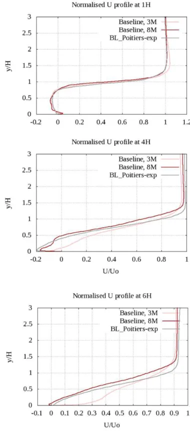
4.3.3.5.2 Velocity profiles ... 118
Table of Contents
Page xi
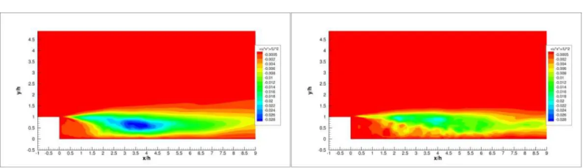
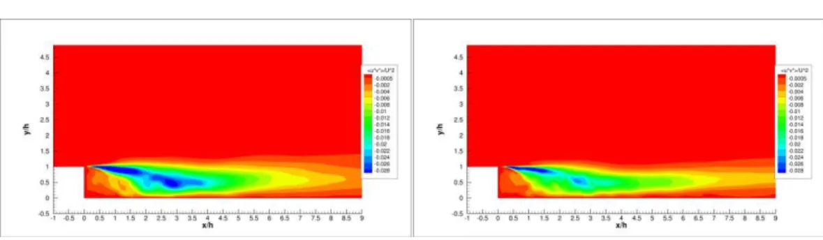
4.3.3.5.4 Reynolds stress ... 123
4.3.4 Three dimensional study: DBD plasma actuation over a backward facing step (Poitiers) applying unsteady actuation of plasma ... 129
4.3.4.1 Analysis of the modulated plasma produced by Singh and Roy’s model and comparison of results against Poitiers experimental database and MARS 3D Shyy’s modulation of plasma results. ... 131
4.3.4.1.1 Analysis of turbulent coherent structures of the flow ... 133
4.3.4.1.2 Velocity profiles ... 135
4.3.4.1.3 Reattachment region and skin friction distribution studies ... 138
4.3.4.1.4 Reynolds stress ... 139
4.4 Conclusions ... 146
5 Active flow control with Spanwise Vortex Generators over a backward facing step ... 151
5.1 Introduction ... 151
5.2 Case Configuration... 151
5.2.1 Description, review and adjustment of the device: passive vortex generators, cavities and blockages and active vortex generators. ... 151
5.2.2 Geometry and Computational Domain ... 154
5.2.3 Boundary Conditions and Time step selection ... 156
5.3 Implementation of Spanwise Vortex Generators in DGDES ... 157
5.4 Results and Discussion: comparison with experimental database ... 157
5.4.1 Analysis of coherent structures ... 157
5.4.2 Velocity profiles ... 159
5.4.3 Reattachment region and skin friction distribution studies ... 161
5.4.4 Reynolds stress ... 164
5.5 Conclusions ... 170
6 Final conclusions ... 171
6.1 Summary of work and achievements ... 171
6.1.1 Single DBD plasma actuation achievements ... 171
6.1.2 Spanwise Vortex Generators actuation achievements ... 173
6.2 Future work ... 173
6.2.1 Suggestions for DBD plasma actuation ... 174
Table of Contents
Page xii
Appendix: Two dimensional simulation of SVG: an exploration of the skin friction coefficient distribution along the streawise direction. ... 177 References ... 179
Page xiii
List of Figures
Figure 2.1 Examples of turbulence in real life ... 8
Figure 2.2 Piezoelectric actuators at the University of Manchester wind tunnel. ... 18
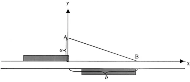
Figure 2.3 Suction/blowing locations on a backward facing step. (A) Bottom corner of step; (B) Step edge; (C) Multichannels along vertical wall of step ... 19
Figure 2.4 Schematics of synthetic jet ... 20
Figure 2.5 Schematics of a DBD plasma actuator ... 21
Figure 3.1 Geometry similarity diagram ... 62
Figure 3.2 Basic principle of an axisymmetric DBD plasma actuator ... 65
Figure 3.3 Plasma visualisation along the spanwise of wind tunnel at University of Poitiers ... 65
Figure 3.4 Triangular area of actuation of plasma in Shyy’s model ... 67
Figure 3.5 Single DBD plasma actuator diagram according to Singh and Roy’s model ... 71
Figure 4.1 Scheme of a flow over a BFS... 76
Figure 4.2 Computational Mesh ... 78
Figure 4.3 Y+: DGDES vs RANS (Fluent) ... 81
Figure 4.4 Velocity streamlines: S-A URANS vs RNG k- ε RANS ... 82
Figure 4.5 Skin Friction Coefficient Distributions ... 83
Figure 4.6 BFS model in wind-tunnel (CNRS PPRIME Poitiers) ... 85
Figure 4.7 DBD plasma actuator configuration ... 85
Figure 4.8 Computational 2D mesh, x-y view ... 86
Figure 4.9 Detail of mesh at step region, x-y view ... 87
Figure 4.10 Baseline streamlines, experimental and simulation respectively ... 88
Figure 4.11 Streamlines and streamwise velocity contours for a set of different CROY constants ... 90
Figure 4.12 Streamlines for steady forcing. Experimental case ... 91
Figure 4.13 Streamlines and U/U∞ contours: Singh and Roy’s and Shyy’s models, respectively ... 91
List of Figures
Page xiv
Figure 4.14 x-y plane of 8M computational mesh (top) and detail of step region (bottom) ... 94 Figure 4.15 Streamlines comparison: 3M versus 8M mesh ... 94 Figure 4.16 Time and spanwise averaged streamwise velocities at three different x/H locations ... 96 Figure 4.17 Normal Reynolds stresses at three different locations... 98 Figure 4.18 Normalised normal Reynolds stresses <u’u’>, <v’v’> and <w’w’> for the 3M mesh –left column- and the 8M mesh –right column- baseline cases ... 99 Figure 4.19 Normalised turbulent shear stress profiles at three locations ... 100 Figure 4.20 Normalised turbulent shear stress, <u’v’> for the 3M mesh –left- and the 8M mesh –right- baseline cases ... 101 Figure 4.21 Iso-surfaces of vorticity magnitude at 30 for (a) coarser and (b) finer meshes ... 102 Figure 4.22 Time-averaged streamlines for 3M and 8M meshes with steady plasma, respectively ... 102 Figure 4.23 Normalised Reynolds stresses <u’u’> and <v’v’> at 1H, 2H and 6H locations. ... 103 Figure 4.24 Normalised normal Reynolds stresses <u’u’>, <v’v’> and <w’w’> for the 3M mesh –left column- and the 8M mesh –right column- steady plasma cases 104 Figure 4.25 Normalised turbulent shear stress <u’v’> at 1H, 2H and 6H ... 105 Figure 4.26 Normalised turbulent shear stress, <u’v’> for the 3M mesh –left- and the 8M mesh –right- steady plasma cases ... 106 Figure 4.27 Iso-surface of vorticity magnitude at 30 for steady plasma using (a) a 3M mesh and (b) an 8M mesh ... 107 Figure 4.28 Time and spanwise averaged streamlines: (a) CROY=7x10
-8, (b)
CROY=2.2x10 -8
, (c) CROY=7x10 -9
, (d) Shyy model, 65% efficiency ... 109 Figure 4.29 Velocity profiles at 1H, 2H and 6H for the three different Singh and Roy’s constants and Shyy model ... 110 Figure 4.30 Normalised Reynolds stresses at 1H, 2H and 6H for three different Roy’s constants, Shyy model and experiment ... 113 Figure 4.31 Normalised turbulent shear stress <u’v’> at 1H, 2H and 6H for three different Roy’s constants, Shyy’s model and experiment ... 114
List of Figures
Page xv
Figure 4.32 Q-criterion of baseline case–left column- and the steady plasma actuation –right column- at (a) 1000, (b) 100,000 and (c) 200,000. Iso-surfaces coloured by streamwise velocity. ... 117 Figure 4.33 Comparison of velocity profiles of baseline cases –simulation and experiments- and steady plasma force – simulation and experiment- at -1H, 0H, 1H, 2H, 4H, 6H, 8H, 10H, 14H ... 119 Figure 4.34 Streamlines of flow field: baseline –left column- and steady plasma actuation –right column- comparison. Top row: simulations; bottom: experimental data ... 121 Figure 4.35 Skin friction coefficient distribution along the streamwise direction. ... 122 Figure 4.36 x-z plane showing inverse skin friction distribution ... 123 Figure 4.37 Comparison of normalised Reynolds stresses <u’u’>, <v’v’>, <w’w’> at 1H, 2H and 6H for baseline and steady plasma ... 126 Figure 4.38 Time and spanwise averaged normalised Reynolds stress contours <u’u’>, <v’v’>, <w’w’> ... 127 Figure 4.39 Comparison of normalised Reynolds shear stress <u’v’> at 1H, 2H and 6H for baseline and steady plasma ... 128 Figure 4.40 Normalised Reynolds shear stress <u’v’> contours (top row: simulations, bottom: experimental data) of uncontrolled – left column- and controlled –right- case ... 129 Figure 4.41 Flow streamlines and normalised streamwise velocity contours for modulated plasma using Roy’s model using three different constants (a) CROY=2.0x10
-8
(b) CROY=3.5x10 -8
... 132 Figure 4.42 Flow streamlines and normalised streamwise velocity contours for modulated plasma using Roy’s model using three different constants (a) CROY=5.0x10
-8
(b) CROY=7.5x10 -8
... 133 Figure 4.43 Q-criterion at 1,000 comparison: Shyy’s model (left) versus Singh and Roy’s model (right) ... 134 Figure 4.44 Q-criterion at 100,000 comparison: Shyy’s model (left) versus Singh and Roy’s model (right) ... 134 Figure 4.45 Iso-surface of vorticity: uncontrolled case (left) and controlled (modulated) case (right) ... 135 Figure 4.46 Normalised streamwise velocity at 1H, 2H, 4H and 6H ... 136
List of Figures
Page xvi
Figure 4.47 Experimental flow streamlines ... 138
Figure 4.48 Streamlines of flow field and Normalised U contours; top– Singh and Roy’s model using two different constants; bottom; Shyy’s model ... 138
Figure 4.49 Skin friction coefficient distribution along streamwise direction comparison of baseline and modulated plasma actuation ... 139
Figure 4.50 Normalised <u’u’> Reynolds stress component at 1H, 2H, 4H and 6H ... 140
Figure 4.51 Normalised <v’v’> Reynolds stress component at 1H, 2H, 4H and 6H ... 141
Figure 4.52 Normalised <w’w’> Reynolds stress component at 1H, 2H, 4H, 6H (simulation data only) ... 142
Figure 4.53 Contours of normalised Reynolds stress components: Shyy’s model (left) and Singh and Roy’s model ... 144
Figure 4.54 Normalised Reynolds shear stress u’v’ component at 1H, 2H, 4H and 6H ... 145
Figure 4.55 Normalised Reynolds shear stress u’v’: Shyy’s model (left) and Singh and Roy’s model ... 146
Figure 5.1 Vortex generator on a wing scheme ... 152
Figure 5.2 Vortex generators on the vertical fin of a Boeing 727-100 ... 152
Figure 5.3 Spanwise Vortex Generator (SVG) setup in NUAA wind-tunnel ... 154
Figure 5.4 Wind-tunnel facilities at Nanjing University of Aeronautics and Astronautics ... 154
Figure 5.5 Schematics of the simulated SVG ... 155
Figure 5.6 Computational mesh and detail of step region when SVG are in operation ... 156
Figure 5.7 Q-criterion of baseline –left column- versus SVG case at (a) 1000, (b) 100,000 and (c) 200,000. Iso-surfaces coloured by streamwise velocity ... 158
Figure 5.8 Normalised velocity profiles at nine different locations. Baseline (simulation and experiment) versus SVG simulation profiles ... 161
Figure 5.9 Streamlines of flow field: baseline –top- and controlled case –bottom .. 162
Figure 5.10 Skin friction coefficient distribution along x/H. Simulations versus experimental data (figure shown only for qualitative comparison) ... 163
Page xvii
Figure 5.11 Comparison of normalised Reynolds stress <u’u’> component at six x/H locations ... 165 Figure 5.12 Comparison of normalised Reynolds stress <v’v’> component at six x/H locations ... 166 Figure 5.13 Comparison of normalised Reynolds stress <w’w’> component at six x/H locations ... 167 Figure 5.14 Time and spanwise averaged Reynolds normal stress contours <u’u>/U0
2, <v’v’>/U 0
2, <w’w’>/U 0
2. Baseline – left- versus SVG –right- cases ... 168
Figure 5.15 Normalised Reynolds shear stress <u’v’> profiles at six different x/H locations ... 169 Figure 5.16 Time and spanwise averaged Reynolds shear stress <u’v’>/U0
2 contour:
Page xviii
List of Tables
Table 3.1 values for the first and second order temporal accuracies ... 36
Table 4.1 B.C. for D&S case. Fluent’s mesh. ... 79
Table 4.2 Comparison of meses for the two different solvers for D&S validation case ... 80
Table 4.3 Reattachment length comparison using two different solvers for the D&S validation case ... 83
Table 4.4 Set of constants for Roy’s model adjustment in 2D cases ... 89
Table 4.5 Singh and Roy’s constants for 3D model adjustment cases ... 108
Nomenclature
Page xix
Nomenclature
Roman SymbolsA (= Ai) Vector of a surface area Ac Conservative Jacobian matrix
C A constant number
CDES A constant in DES
Cf Coefficient of skin friction ci, c Speed of sound
cp Specific heat capacity at constant pressure CROY Constant applied to Singh and Roy’s model cv Specific heat capacity at constant volume d Length scale in hybrid RANS/LES techniques
Wall distance, the distance from a point to the nearest wall E Specific total energy
E
Electric fielde Electron charge
f Flow control frequency Constants in DES
Blending/damping function
Fx0, Fy0 Constants in Singh and Roy’s model
F Vector of convective flux
Fd Vector of dissipation flux in the Roe scheme
G Vector of viscous flux
H Specific total enthalpy or height of the step in BFS K Parameter in Roe’s scheme
k Specific kinematic energy or turbulence kinetic energy k1, k2 Constants in Shyy’s model
Nomenclature
Page xx
l Length of eddies
LLES LES length scale
lhyb Hybrid length scale of turbulence and RANS average lRANS RANS length scale
lturb Turbulence length scale
M Mach number
n (= ni) Normal vector of a surface, i = 1, 2, 3 Nface Face number
nr A random number with magnitude less than a unity Nz Cell number along a span
p Fluid static pressure Ap Primary Jacobian matrix
Pr Prandtl number
Q Vector of primary variables, Q = (p, u1, u2, u3, T)T q (= qi) Heat flux vector, i = 1, 2, 3
R Residual vector in the N-S equations
r Adisplacement vector form one point to another R The ideal gas constant for air, R = 287.04 J Kg−1 K−1
Re Reynolds number
S Source term in Navier-Stokes equations
S
(= Sij) Rate of strain tensor, or a vector of the source term in the N-S equationsT Fluid absolute temperature
t Physical time
T0 The reference temperature in the Suntherland’s law, T0 = 273.11
K, or a time interval ∆t Physical time step
∆t∗ Dimensionless time step, ∆t
∗
= ∆t/(L/U∞) TFT Flow-through time periodNomenclature
Page xxi
u (= ui) Velocity vector, i = 1, 2, 3 U∞, U Free stream velocity
un The real normal velocity of a surface of a control volume, un = (u - ug) · n
uτ Friction velocity, = ( / )
u’u’, v’v’,w’w’ Normal Reynolds stress components u’v’, u’w’, v’w’ Reynolds shear stress components
u, v, w Instantaneous velocity components in Cartesian coordinates
V Volume of fluid
W Vector of conserved variables XR Reattachment length after the step x, y, z Cartesian coordinates
Greek Symbols
α Thermal diffusivity
Coefficients in physical term discretisation using backward Euler scheme
Parameter in AUSM
β Parameter in AUSM
βx, βy Dielectric constants used in Singh and Roy’s model δ Boundary layer thickness
δij Kronecker’s delta symbol
∆τ Pseudo time step
∆x Characteristic length of a control volume
ϵ Energy dissipation rate, or a small number
Frequency of applied AC voltage in Shyy’s model
Φ0 Applied voltaje in Singh and Roy’s model η Kolmogorov’s length scale
γ Heat capacity ratio, = /
Nomenclature
Page xxii
Γnc A transition format of the transformation matrix in the
preconditioning
κ Von Karman constant, κ = 0.41 Thermal conductivity coefficient
λ Bulk elasticity or second coefficient of viscosity, or spacial interval between two adjacent jets
Λ (= λk) Diagonal matrix of eigenvalues, k = 1, 2, ...5 Λc Spectral radii of the convective flux
Λv Spectral radii of the viscous flux
µ Dynamic viscosity
µ0 The reference viscosity in the Suntherland’s law, µ0 = 1.716×10 −5
m−1 Kg s−1
ν Kinematic viscosity
νt Turbulent kinematic viscosity Ω (= Ωij) Vorticity tensor
ω Specific dissipation ratio in k- ω turbulence model
ω
(= ωi) Vector of angular velocityΨ A low-Reynolds number correction in DES and its variations
ρ Fluid density
Van Neumann number
τ Pseudo time
τi,j Reynolds stress tensor
τij|mod The modelled Reynolds stresses τij|res The resolved Reynolds stresses τij|TOT The total Reynolds stresses
Θ A replacement of ρp in the preconditioning
ε Coefficients in the backward Euler’s discretization Dissipation of turbulence kinetic energy
Nomenclature
Page xxiii
Superscripts
+ Dimensionless distance, ≡ /
L The left side of a surface
M Modelled variables
m Time step of the pseudo time n Time step of the physical time
′ Flow fluctuation
R The right side of a surface, or the Reynolds Averaged variable S Sub-grid scale filtered variable
T Transposition of a vector or a matrix
Subscripts exp Experimental data
i i = 1, 2, 3 corresponds to Cartesian coordinates, x, y, z j j = 1, 2, 3 corresponds to Cartesian coordinates, x, y, z m Measured variables in experiments
Other Symbols
∙̂ Roe averaged values
〈∙〉 Spatial averaged
∙̅ Time averaged
∙̃ Modified variables in the S-A model
∇ Local mesh spacing
Nomenclature
Page xxiv
Acronyms
2D Two Dimensional
3D Three Dimensional
ALE Arbitrary Lagranigan-Eulerian
AUSM Advection Upstream Splitting Method BFS Backward Facing Step
CFD Computational Fluid Dynamics
CFL Courant-Friedrichs-Lewy condition or number DBD Dielectric Barrier Discharge
DES Detached Eddy Simulation
DDES Delayed Detached Eddy Simulation
DGDES Dynamic Grid Detached Eddy Simulation in-house code DNS Direct Numerical Simulations
EHD Electro-hydro-dynamic plasma force FVM Finite Volume Method
GCL Geometric Conservation Law
IDDES Improved Delayed Detached Eddy Simulation LHS Left Hand Side
LES Large Eddy Simulation
MARS Manipulation of Reynolds stress for Separation Control and Drag Reduction
MPI Message Passing Interface platform for core’s communication
N-S Navier-Stokes
NUAA Nanjing University of Aeronautics and Astronautics RANS Reynolds-Averaged Navier-Stokes
RHS Right Hand Side
Nomenclature
Page xxv
SGS Sub-grid Scale
SLAU Simple Low-dissipation Scheme of AUSM-family SST Shear Stress Transport turbulence model
SVG Spanwise Vortex Generators
URANS Unsteady Reynolds-Averaged Navier-Stokes WMLES Wall-Modelled Large Eddy Simulation
Introduction
Page 1
1
Introduction
1.1
Background and motivations
The manipulation of a flow field, widely known as flow control, by means of active or passive devices has been a subject of high importance throughout the history of Fluid Mechanics. The changes introduced in the flow are basically related to investigating their effects in flow separation control, skin friction and drag reduction, laminar to turbulent transition investigation and so on.
Numerous methods have been developed since the beginning of the XX century up to nowadays. Passive control implies the introduction of changes with regards to the variation of the geometry of the domain of the flow. On the other hand, active control includes the introduction of external energy into the flow field to change the original flow field as it will be later explained.
Drag reduction and separation control are directly related to more efficient air transportation and less emission of harmful gases into the environment. While the aerospace industry is striving to have more and more optimised designs, it is still some way away from the targets set out in the ACARE 2020 vision for 50% reduction in aircraft emissions. Separation control and drag reduction contribute directly towards this target and active flow control could play an important role in achieving it. Active flow control provides an additional dimension for further improving aircraft performance, in particular, for performance at different operational points, such as at cruise and take-off and landing. After many decades of development, the highly optimised aircraft designs make further large improvements difficult without a game changing technology such as active flow control.
Going deeper into the concept, the turbulent Reynolds stress is the most important dynamic quantity affecting the mean flow as it is responsible for a major part of the momentum transfer in a wall bounded turbulent flow. It has a direct relevance to both skin friction (for a turbulent boundary layer) and flow separation (occurs when skin friction drops to zero). The near wall region for a turbulent boundary layer can
Introduction
Page 2
be divided into the viscous sub-layer, where the mean viscous stress is important; and the approximately constant Reynolds stress region where the viscous stress drops to zero and the Reynolds stress peaks. As the Reynolds number increases, the peak Reynolds stress approaches the value of the viscous stress at the wall. Therefore active manipulation of the Reynolds stress can directly lead to changes in the viscous stress at the wall so as to effectively control the flow.
Active flow manipulation is directly related to control of separation and a reduction of the drag yielding to more efficient air transportation and to eco-friendlier aircraft performance reducing the emission of harmful gases to the atmosphere.
The capability to control individual flow structures that are larger in scale and have lower frequency compared to the richness of the time and spatial scales in a turbulent boundary layer will be demonstrated. This thesis analyses two novel active flow control means: a dielectric barrier discharge plasma actuator and spanwise vortex generators. To explain the basic strategy in manipulating Reynolds stresses through the dynamic components of the turbulent shear layers, it is helpful to start with the triple decomposition proposed by Reynolds and Hussain, 1972, for an instantaneous velocity, , where
= + " + ′
The first term on the RHS is the time averaged mean velocity. If we attempt to control this via flow control then most devices offer little gain in efficiency on a global energy basis, i.e. change in energy out is equal to energy in. The second term on the RHS is the periodic/dynamic component of the flow and for some specific flow scenarios this can be shown to be dominant in determining the flow state and characteristics. The stresses produced from this term are referred as the periodic stresses. It offers some interesting opportunities for demonstrating the way in which to deploy flow control technologies for dynamic environments (responsive environments, smart inputs and sensible control). This also implies that, for statistically steady flows where the second term disappears, artificial introduction of the periodic term may be necessary for effective control. The final term on the RHS represents the broadband “random” turbulent fluctuations from which the Reynolds
Introduction
Page 3
stresses are defined. Whilst direct control of the “random” components is the ultimate goal, the current project aims to investigate the control of the periodic stresses, the dynamic components of the flow, in order to manipulate the Reynolds stress for the benefit of flow control.
Different types of flow control have been widely investigated during the past two centuries [Prandtl, 1904; Schubauer and Skramstand, 1947; Gad-el-Hak and Bushnell, 1991; Choit et al., 1994; Gad-el-Hak, 1998, 2003]. As mentioned before, flow control devices can be classified into passive and active flow control devices. Passive flow control comprises changes in the geometry via the installation of devices such as the classic vortex generators which will create or destroy large turbulent structures of the flow. Active flow control, on the other hand, introduces energy into the flow field from external devices such as moving or oscillating surfaces, synthetic jets, etc., and consequently the original flow field is perturbed.
Passive devices offer a limited effectiveness on flow control as they are operational in a single or small range of operation points whereas active flow control offers a much broader possibility of development by investigating the techniques to enhance their ability to control turbulent flows in a wide variety of configurations and applications. By understanding the interaction of the flow control devices and the resulting flow field, a deeper insight into the effectiveness of active flow control can be achieved. Within the Manipulation of Reynolds stress for Separation Control and Drag Reduction, MARS, project an investigation of flow control devices to enhance the performance of such devices was carried out in order to achieve an improvement of aircraft performance. In this project, an active collaboration of experimental and numerical partners allowed a further understanding of a wide range of flow control devices to reduce skin friction and manipulate Reynolds stress. Two different test cases were chosen to study the effects of various flow control devices. This thesis focuses on the flow over a backward facing step, BFS, and the aforementioned investigated flow control devices were a single dielectric barrier discharge plasma actuator and spanwise vortex generators.
Introduction
Page 4
In order to analyse and research these devices, thanks to the development of technology during the current and past centuries, different computational techniques and tools have been developed. Therefore, the numerical investigation by means of such methods will provide a much better understanding of the effects of active flow control devices which will potentially have an application in real life, leading to development of the current devices, the introduction of new ones and optimisation of their realistic configurations. The final and ultimate motivation is the achievement of more efficient, safer and greener performance of the different means of transport in the aerospace industry.
1.2
Aims and objectives of this work
This thesis was defined and performed as a part of the MARS project hence the objectives are directly related to this project’s goals. The global aims for this study can be defined as,
- To validate via simulation and comparison the implementation of a single DBD plasma actuator and spanwise vortex generators into the in-house code DGDES performing CFD URANS and IDDES simulations.
- To investigate the relation of discrete dynamic structures generated by a single DBD plasma and SVG flow control devices installed on a backward facing step flow and the configuration of these two devices.
- To simulate and understand the impact of the devices on the turbulent structures of two different cases of a flow over a BFS and their effects on the turbulent shear layer to obtain a reduction of the separation region.
- To establish the relation –if any – between the control parameters of the devices and the resulting Reynolds stress and skin friction distribution.
1.3
Outline of the thesis
In this study, several 2D RANS and URANS and 3D IDDES are performed to prove the consistency and reliability of such simulations as all of the calculations will be validated and compared to two different experimental databases. For the single DBD plasma actuator, simulations are carried out according to the setup of the experimental partner from the University of Poitiers. Secondly, the spanwise vortex generators case will be compared and simulated following the configuration from
Introduction
Page 5
Nanjing University of Aeronautics and Astronautics. Both experimental partners also contributed with their work for the MARS project.
A brief outline of the chapters is given here:
• Chapter 1: In this current chapter, the background and motivations and the
objectives and aims are presented. A brief introduction to the two main chapters of this thesis is also provided.
• Chapter 2: The main features of turbulence and its modelling approaches
and the most popular active flow control devices are described and presented.
• Chapter 3: A full description of the governing equations and how the flow
solver DGDES works is given in this chapter. The methodology and numerical schemes are described. Moving mesh techniques and plasma models implementation into the in-house code are described.
• Chapter 4: The complete plasma actuation study carried out for this thesis is
provided. First of all a comparison of the solver DGDES is performed against a 2D calculation using a commercial code. Then, the case from Poitiers where the plasma device was experimentally investigated is analysed. First of all, 2D study for initial Singh and Roy’s model validation is carried out. Once the model is adjusted, several three dimensional studies are performed to validate the model completely. A mesh dependency study is performed for both baseline and plasma actuation cases to choose a proper mesh for the investigation. An eight million cells grid is selected for further investigation of Poitiers case as it shows closer results to the experimental data. A series of Singh and Roy’s constants are then tested and compared to the data from the experimental partner and a final assessment with the final selected constant for steady and unsteady plasma actuation is shown. Final overall conclusions are also included in this chapter.
• Chapter 5: The second flow control device study is presented in this chapter.
A description of the experimental facilities for the investigation of the spanwise vortex generators in NUAA is firstly done. The mesh for this case is the eight million cells mesh which was utilised for the DBD plasma study
Introduction
Page 6
as it showed very good results. Both uncontrolled and controlled cases are analysed and compared to the available experimental data. The SVG setup and simulations are then described and the analysis of the coherent structures of the turbulent flow, velocity profiles, reattachment length comparison with the baseline and experimental case is included in this chapter. The conclusions of the investigation are finally presented.
• Chapter 6: A final assessment of the work conducted in the thesis is given in
this chapter. Achievements are discussed and several ideas and proposals for future work involving DGDES, the plasma actuator and the SVG are provided.
• Appendix: Two different 2D simulations, uncontrolled and controlled, were
carried out to explore the skin friction distribution along the streamwise direction for the baseline and controlled cases with the spanwise vortex generators.
Finally, the References part contains the most relevant books and technical papers for this research.
Literature Review
Page7
2
Literature Review
2.1
Introduction
In this chapter the basics of turbulence and its modelling and the active flow control devices used to perform the numerical simulations carried out for the completion of this thesis will be introduced among some other flow control devices.
In order to solve the turbulent flow behaviour accurately, first of all, one must understand the nature of turbulence and its different ways of modelling. A brief explanation regarding the different available methodologies will be given, from the Reynolds Average Navier Stokes (RANS) method to the most complex, Direct Numerical Simulations or DNS. In this work the main technique for resolving turbulence was the hybrid RANS/LES procedure.
Secondly, what active flow control is and how it is been achieved will be described including the active flow control devices which have been investigated in this thesis, i.e., dielectric barrier discharge, DBD, plasma actuators and spanwise vortex generators, SVG. Only a theoretical explanation is given, its modelling and implementation in the computational code will be analysed later on in this thesis.
2.2
Turbulence: definition and modelling
2.2.1
What is turbulence
In this study, the flow was always considered turbulent therefore an explanation of its nature and main features will be given.
Turbulence is a property of a flow not of a fluid: the same fluid can produce laminar or turbulent flows depending on the flow characteristics. Also, and before going any deeper into turbulence and its characteristics, it is really important to clarify that turbulence is a continuum phenomenon: even the smallest turbulent scales are larger than molecular scales. Even though the vortices distribution in a turbulent flow is highly irregular, it is continuous.
Literature Review
Page8
In order to assess whether a flow is laminar or turbulent, the Reynolds number is used. This number is a non-dimensional parameter defined as the ratio of inertial to viscous forces. When Reynolds number is a small number, the flow is strongly characterised by viscous effects, therefore instabilities are suppressed by the viscosity. In fluid mechanics, a laminar flow occurs when a fluid flows in parallel layers, with no disruption between the layers. At low velocities, the fluid tends to flow without lateral mixing and adjacent layers slide past one another like a deck of playing cards. Laminar flow is characterised by high momentum diffusion and low momentum convection.
Figure 2.1 Examples of turbulence in real life
On the other hand, when a flow is characterised by a high Reynolds number, there is a high interaction between diffusive –viscous- terms and convective –inviscid- terms and the flow is remarkably rotational and irregular with an increase of instabilities as a consequence, and it is known as turbulent flow. So in reality, most of flows present in real life are turbulent, Fig. 2.1, from the smoke of a candle to the flow of a river or the wake of an airplane. All these flows are found to be highly non-linear characterised by a chaotic and stochastic behaviour of the fluid itself. The flow contains eddies which result in lateral mixing with a rapid variation of velocity and
Literature Review
Page9
pressure both in space and time. The properties of a turbulent flow vary in a random way. Hence, it is really difficult to provide an accurate definition for turbulence. Nevertheless, turbulence can be highly characterised by the following points:
- Irregularity: turbulent flows are very irregular. That is why turbulence is always treated statistically: a turbulent flow is unique and it will never be repeated in the exact same way in nature.
- Diffusivity: In turbulent flows, the mixing is improved due to the available supply of energy in them. Turbulent flows enhance the mixing and also increase the rate of mass, momentum and energy transports.
-Rotationality: In turbulent flows, three dimensional vortex stretching is always present and the flow has vorticity, i.e., the turbulence is always 3D rotational. Vortex stretching is responsible of the turbulence energy cascade phenomena where unsteady vortices appear and interact with each other. The stretching mechanism makes the vortices go thinner due to the volume conservation of fluid elements, therefore the larger vortices break down into smaller flow structures until these small structures are small enough so their kinetic energy is overwhelmed by the fluid’s molecular viscosity and dissipated in heat form. [Batchelor, 1953; Pope, 2000]
- Energy cascade: Turbulent flows are a continuum phenomenon and they contain a wide variety of scales of motion. The energy cascade occurs from the largest scales to the smallest scales. The largest scales are responsible for the transport and generation of turbulence whereas the smallest scales dissipate the energy coming from the larger scales into internal energy in form of heat as mentioned previously. Consequently, turbulence flows can be interpreted as a superposition of eddies with a wide range of uncontrollable and non-symmetric length scales upon a mean flow. Velocities have also random fluctuations. The hierarchy from bigger eddies to the smallest ones is determined by the energy spectrum which measures the energy in the fluctuations of the velocity for each wave number. According to this, length scales are divided in three categories. In first place, the largest scales in the energy spectrum are known as integral length scales. Eddies obtain the energy from the mean flow and also from each other. They have low frequencies and large velocity fluctuations. Taylor
Literature Review
Page10
microscales are the intermediate scales. They pass energy from the largest scales to the smallest and they are not dissipative. And finally, the Kolmogorov length scales are the smallest scales in the spectrum. They have high frequencies and lower velocity fluctuations. In this range of the energy spectrum, the energy drain from viscous dissipation and energy input from nonlinear interaction are in balance.
- Dissipation: Turbulent flows are highly dissipative. Viscosity effects at smallest scales result in the conversion of kinetic energy of the flow into hear or internal energy. Accordingly, in order to maintain a turbulent regime a constant supply of energy is required.
2.3
Modelling turbulence
As discussed in the previous section, an exact definition for turbulence cannot be given; consequently when a simulation of a turbulent flow is going to be performed models are needed to represent the scales of the flow which cannot be resolved due to their unpredictable behaviour. In order to solve aerodynamic problems numerically, the mathematical solution of the equations of motion for fluid flow can be obtained for a wide range of different cases. Different techniques have been developed derived from Navier-Stokes equations. The computational fluid dynamics, CFD, approach chosen for a particular case depends on which accuracy the solution of the problem requires and also it depends on the high performance computing resources available in terms of computational time and cost.
A description of the main approaches will be provided in the next sections: from the less demanding Reynolds-averaged Numerical Simulation, RANS, approach to the Direct Numerical Simulation, DNS, and the approaches in between.
2.3.1
Reynolds-averaged Navier-Stokes equations Modelling (RANS)
RANS approach is the most common used to solve the real life flows by applying the statistical mean average directly to the solution: the flow is resolved in terms of time and space averaged variables only by means of the Reynolds averaging method, where every variable in the Navier-Stokes equations is decomposed in a mean quantity and its fluctuating component over time,Literature Review
Page11
(#$, &) = (#(((((((( +') )(#$, &) (2.1)
This decomposition results in an equation for the average flow variables, ((((((((, (#') and additional fluctuating quantities, )(#$, &), known as Reynolds stresses. These stresses represent the momentum transfer due to the fluctuations to the mean flow. Reynolds stresses are characterised by its randomness nature and therefore, the resulting equations need to be closed by using turbulence models. RANS can be seen as an approach where turbulent scales are not resolved but all the turbulence effects on the mean flow are modelled. This approach requires less computational time and provides decent solutions of the turbulent flows in the near wall region. However, when a not statistically stationary flow is going to be resolved, RANS does not provide an accurate solution as in this approach the flow is considered to be steady [Iaccarino, 2003]. A variation of RANS called unsteady RANS or URANS would be applied in such case. URANS introduces a new term in the variables decomposition known as phase-average or conditional statistical average term. This quantity represents the coherent behaviour in the flow dynamics. When the flow is periodic in time, an URANS simulation must be averaged over one period in order to be able to compare with time-averaged data. Despite the time dependence and large vertical structures, URANS is not a simulation of the turbulence, only of its statistics. A definition of URANS is given by Merzari et al. (2009), based on the ensemble averaging over different realisations of the flow fields. URANS is regarded as a generalised filter in both time and space with characteristic filter spatial scales and filter temporal scales.
2.3.2
Large Eddy Simulations (LES)
LES resolves the large scales of the turbulent flow and the rest of smaller scales are modelled using a subgrid scale (SGS) model which statistically affects the large scale motion of the flow. In a turbulent flow, the major part of energy and momentum transfer to the mean flow is mainly caused by the larger scales of the flow into the smaller scales; for such reason, this method turns out to be very interesting from the engineering point of view. Computationally speaking LES is more demanding than RANS but less demanding than DNS, but also it is expected to be more accurate as it
Literature Review
Page12
resolves the large scales directly. In LES all the scales with size smaller than the grid size are filtered and will be modelled afterwards. Filtering the Navier-Stokes equations means basically to remove eddies smaller than the filter, usually defined by the grid size. All these removed eddies will be the modelled part of LES approach and this modelling is the necessary closure for the approach. Bearing this in mind, the total velocity field will be the result of the sum of the resolved velocity field and the modelled component.
Different subgrid scales, SGS, models can be used. The first model used for LES filtering was the Smagorinski model, [Smagorinsky, 1963]. The applied constant in this model was estimated from isotropic homogeneous flows and it results in a highly dissipative model for most of real but simple flows. Later on, in order to sort this problem out Germano et al. (1991) proposed a variation to the Smagorinski model by using two filters instead of one to calculate the Smagorinski coefficient dynamically based on local transient flow fields.
In the past years, many different SGS models were proposed such as wall-adapting local eddy-viscosity model [Nicoud and Ducros, 1999], where a spatial filter related to the wall distance and cell volume was introduced and it guaranteed a zero turbulent viscosity for laminar shear flows or one of the most recent models by You and Moin (2007) who proposed a method which can be used in complex geometries.
2.3.3
Direct Numerical Simulations (DNS)
DNS is by far the most complex technique when resolving an aerodynamic problem. Direct Numerical Simulations, as its own name indicates, provides a complete description of turbulent variables and resolves Navier Stokes equations directly without any modelling. The whole range of turbulent scales, from the large scale eddies to the Kolmogorov dissipative scales, is resolved.
In order to capture all the turbulent length scales numerically, both time step and grid space sizes must be smaller than the smallest eddy sizes, the Kolmogorov scales and its characteristic time scales. DNS simulations are, therefore, highly demanding in time and computation costs. For this reason, the applicability of this technique is limited to low Reynolds number flows and other approaches such as the previously
Literature Review
Page13
described RANS and LES and the following described in the next sections were developed to be able to tackle the turbulent flow problems at high Reynolds numbers.
2.3.4
Hybrid RANS/LES techniques
In this section, different hybrid RANS/LES methods will be described. A deeper analysis of these approaches will be made as this work is based in hybrid RANS/LES computations. These techniques were designed to combine the best aspects of RANS and LES approaches. Regarding RANS, its best aspect taken is the near wall region/boundary layer treatments and regarding LES its features when tackling separated flows were taken for the different hybrid approaches. As discussed previously, LES requires a very fine mesh near the walls and a high computational cost, but RANS can be applied close to the wall as a feasible method at high Reynolds number cases and LES would be applied away from the walls, resolving the large scales of the flow.
Detached Eddy Simulation, DES, is one of the most widely used hybrid RANS/LES approaches. It was firstly proposed by Spalart et al (1997). It was initially developed to be applied in high Reynolds number flows where a massive separation occurs, such as aerospace and ground transportation problems.
Essentially, it “senses” the grid density and compares the grid spacing in all directions in order to assign the near wall region to RANS and SGS model in the rest of regions. It can be defined then as “a three-dimensional unsteady numerical solution using a single turbulence model, which functions as a subgrid-scale model in regions where the grid density is fine enough for a LES simulation and as a Reynolds-averaged model in regions where it is not” [Shur et al., 1999]. Therefore, the boundary layer would be treated by RANS and regions with massive separation would be treated by LES. The space between these two areas, known as the grey area, may be problematic as it has to be wisely decided when to switch to RANS or LES, but this issue will be addressed later in this section.
DES proposed by Spalart et al. is based in the Spalart-Allmaras one-equation turbulence model, [Spalart, 1992]. In RANS mode, the length scale, *, is defined as
Literature Review
Page14
the shortest distance from any point to the closest wall in RANS model. In DES, * is replaced as the minimum distance from the wall to the length proportional to the local mesh spacing, ∇,
*+,- = min (*, 1+,-∇) (2.2)
where 1+,- is a constant which can take different values but 0.65 is the most common. [Shur et al, 1999].
The local grid spacing will be dependent on the type of mesh: when using a structured mesh, ∇ will be the maximum grid spacing over the three directions x, y, z. If, on the other hand, an unstructured mesh is used, ∇ will be the maximum edge length connecting the centroids of the neighbouring cells. DES will be in RANS mode using Spalart-Allmaras turbulence model when *+,- = * and will be operating in LES mode otherwise, using the Spalart-Allmaras as the subgrid scale model. There is a problem known as the grey area in this hybrid approach. DES only depends on the grid and length scales and when a mesh refinement is performed, it may trigger to LES mode when the boundary layer is fully attached: when the grid spacing parallel to the wall is less than the boundary layer thickness, the LES method takes over as the length scale is fine enough for the detached eddy simulation to switch into a LES model from RANS mode; however, the grid spacing is partially inside the boundary layer and the resolved Reynolds stresses in LES mode do not completely replace the modelled Reynolds stresses from the RANS mode. This leads to a depletion of the stresses which in turn leads to an over prediction of the separation area producing a reduction of the skin friction computation which is not physically real, [Panguluti, 2007]. In order to solve the grey area issue, different variants of the DES were developed. A deeper explanation will be provided in the next Chapter of this thesis.
Literature Review
Page15
2.3.5
RANS, LES or DES?
To close section 3 of this chapter, a brief assessment of RANS, LES and DES simulations will be given. Nowadays, it is well-known that RANS performance is not able to produce accurate results when it comes to problems which imply massive separations. Due to this lack of success, researchers have applied other flow techniques to resolve the dynamics of the flow such as LES or even DNS. However, these other techniques are still computationally too expensive as it has already been commented previously in this work.
Regarding LES, it was shown by Spalart et al. (1997), that for flow simulations in which Reynolds number was about 107 a grid of 1011 cells would be necessary in
order to obtain a sufficiently accurate solution of the problem. Although computers are in constant development, a grid of such number of cells is still too expensive in the sense of computational requirements. This situation gave place to the beginning of development of hybrid RANS/LES techniques.
Breuer et al. (2003) made a comparison of three different approaches such as DES, RANS and LES for a separated flow around a flat plate at high incidence was carried out.
It was soon shown that RANS due to its time-averaged characteristics has got a lack of resolving the unsteadiness of massively separated flows and then it can be concluded that RANS is not able to produce reliable results as it lacks to reproduce the unsteady characteristics of the separated flow field. LES, on the other hand, provides good and reliable results when facing separated flows as it resolves the larger structures of the flow and models the smaller turbulent structures after the SGS filter is applied. However, and it is worth mentioning it again, it is an expensive computational technique as it demands a really fine mesh to predict the resolved turbulent structures. And finally, DES the hybrid RANS/LES method combines the best features of the two approaches: near the walls within the boundary the flow is solved via RANS and a turbulence model such as Spalart-Allmaras is applied and in the rest of the domain where the bigger turbulent structures are present a LES simulation is performed. Therefore, the application of hybrid RANS/LES is appropriate and recommended when the problem to solve consists of unsteady
Literature Review
Page16
turbulent flows with large separation regions. The two cases analysed in this thesis accomplish such condition: when the flow of air moves over the backward facing step, a massive separated bubble occurs after the step and in order to achieve accurate and computationally affordable simulations, a variant of DES was the approach chosen for this study. Furthermore, certain issue –the aforementioned grey area problem- was found when using DES, but this will be addressed in Chapter 3, in which a deep analysis of DES and its variants is provided.
2.4
Flow Control
As a basic concept, it is well-known that drag reduction and separation control are directly related to more efficient air transport with a lower emission of harmful gases into the environment. Separation control and drag reduction contribute directly towards greener aircraft efficiencies and active flow control plays a vital role in achieving it.
Reynolds stress is the dynamic quantity responsible for transferring the majority of momentum in a wall bounded flow. Hence, it has a direct influence into both skin friction and flow separation. It was said in the introduction of this thesis that in the viscous sublayer of the turbulent boundary layer in the near wall region the mean viscous stress is definitely more influent on the flow than the Reynolds stresses and in the constant Reynolds stress region, the viscous stress drops to zero and the Reynolds stress peaks. Increasing the value of the Reynolds number, the peak Reynolds stress approaches the value of the viscous stress at the wall. For this reason, an active manipulation of the Reynolds stress can directly lead to changes in the viscous stress at the wall so as to flow control.
However, there is a lack of current understanding of the inter-relationship between the various flow control devices such as piezoelectric oscillating surfaces, synthetic jets, dielectric plasma actuators, oscillating vortex generators, etc., and the Reynolds stresses in the flow field these devices generate. A better understanding can potentially and significantly improve the effectiveness of flow control as the Reynolds stresses are closely related to the flow behaviour at the surface for effective separation control or drag reduction. A variety of control devices are available and new ones are invented but which one for what purpose is an open question yet to be
Literature Review
Page17
fully answered. The vast majority of previous work so far has focused on the introduction of changes to the mean flow that resulted in changes to the Reynolds stress. In this thesis, it is proposed to reverse that process and consider the long term goal of controlling dynamic structures that then influence the Reynolds stress that in turn change the mean flow. This radical approach recognises that we are still away to implement the concept at flight scales but it is an aim to establish a first important step towards this ultimate ambition. The focus of the present section will be on describing the different types of actuators and the types of flow control. The complete explanation of these two active flow control devices investigated in this thesis is fully contained in Chapter 4 and Chapter 5 where their effects on the discrete dynamic components of the turbulent shear layer and the Reynolds stress will be discussed.
There are two possible ways of flow control: passive and active. Passive control implies no input of energy into the flow but it is modified by placing fixed physical devices into the geometry such as vortex generators, riblets, surface roughness, bumps, cavities and so on. The other kind of control is known as active control, where there is an external form of energy introduced into the flow to manipulate its state. All the work carried out in this thesis is only focused on active flow control. With regards to actuation, active flow control devices are nowadays locally applied and their only requirement is an electrical power input. Seifert et al (1996) showed that separation control using periodic addition of momentum at frequencies a bit higher than the natural frequency of the vortex shedding of a flow could produce similar performance improvement as when a steady blowing actuation is applied. There are different types of active flow control devices such as,
- Piezoelectric actuators: These devices are installed normally along the spanwise direction of the surface of the studied geometry, such an aerofoil or wall. Fig. 2.2 shows the configuration of piezoelectric actuators in a wind tunnel at the University of Manchester for the MARS project, [Wang et al, 2014]. The piezoelectric actuators are excited by an electric current and as a result the device behaves as an oscillating surface enhancing the flow
Literature Review
Page18
momentum in the boundary layer and suppressing the turbulent intensity. [Wang, 2013].
Figure 2.2 Piezoelectric actuators at the University of Manchester wind tunnel.
- Suction/blowing devices: These devices consist of nozzles where either constant suction or blowing affecting the boundary layer is performed. Different suction/blowing velocities will produce different effects on the air flow. Different configurations and locations of the nozzles/slots/slits in a backward facing step can be found in the literature. The slots can also have different shapes such as rectangular, triangular/serrated [Uruba et al, 2007] or circular shapes. With regards to the location of the slots, a typical and widely seen configuration is at the bottom of the step on the vertical wall, Fig.2.4(A),[Sakuraba et al 2004; Uruba et al, 2007; Bakhshan et al, 2012]; also the slit is typically located at the edge of the step, Fig.2.4(B) [Chung, 1996; Yoshioka et al, 1999, 2001; Dejoan, 2004; Mehrez, 2010]. Multichannel cases can also be configured such as the location of multiple slots along the vertical wall of the step, Fig.2.4(C) [Emami-Naeini et al, 2006].
Literature Review
Page19
Figure 2.3 Suction/blowing locations on a backward facing step. (A) Bottom corner of step; (B) Step edge; (C) Multichannels along vertical wall of step
- Synthetic jets: These devices are a sort of zero-net mass flux jets which means the working fluid is used without any external mass source or sink. This actuator consists of a series of orifices placed along the streamwise direction of the geometry. Inside the nozzles there is a chamber where there is a membrane oscillating at a certain amplitude and frequency generating a suction/blowing effect at the exit of the nozzle, Fig 2.4, [Ming, 2013]. Another configuration could be where instead of a membrane oscillating, there is a moving wall producing the synthetic jet effects [Cadirci and Gunes, 2012]. Different simulations have been carried out with regards to this device. The jet direction can be in the streamwise direction of the flow [Valencia, 1997; Dandois et al, 2007] or perpendicular to the flow direction, [Okada et al, 2009].