Randomized Binary Search Trees

(1)

CONRADO MART´INEZ AND SALVADOR ROURA

Universitat Polite`cnica de Catalunya, Barcelona, Catalonia, Spain

Abstract. In this paper, we present randomized algorithms over binary search trees such that: (a) the insertion of a set of keys, in any fixed order, into an initially empty tree always produces a random binary search tree; (b) the deletion of any key from a random binary search tree results in a random binary search tree; (c) the random choices made by the algorithms are based upon the sizes of the subtrees of the tree; this implies that we can support accesses by rank without additional storage requirements or modification of the data structures; and (d) the cost of any elementary operation, measured as the number of visited nodes, is the same as the expected cost of its standard deterministic counterpart; hence, all search and update operations have guaranteed expected cost

2(logn), but now irrespective of any assumption on the input distribution.

Categories and Subject Descriptors: E.1 [Data Structures]; F.2 [Analysis of Algorithms and Problem Complexity]

General Terms: Algorithms, Theory

Additional Key Words and Phrases: Balanced trees, probabilistic algebraic specification, randomized data structures, search trees, self-organizing data structures

1. Introduction

Given a binary search tree (BST, for short), common operations are the search of an item given its key and the retrieval of the information associated to that key if it is present, the insertion of a new item in the tree and the deletion of some item given its key. The standard implementation of searches and updates in unbal-anced BSTs is (except for deletions) simple and elegant, and the cost of any of these operations is always linearly bounded by the height of the tree.

Forrandom binary search trees, the expected performance of a search, whether successful or not, and that of update operations is 2(log n) [Knuth 1973; Mahmoud 1992; Sedgewick and Flajolet 1996], with small hidden constant factors involved (here and unless otherwise stated,n denotes the number of items in the tree or size of the tree). Random BSTs are those built using only random

This research was supported by the ESPRIT BRA Project ALCOM II, contract #7141, by the ESPRIT LTR Project ALCOM-IT, contract #20244, and by a grant from CIRIT (Comissio´ Interdepartamental de Recerca i Innovacio´ Tecnolo`gica).

Authors’ addresses: Departament de Llenguatges; Sistemes Informa`tics, Universitat Polite`cnica de Catalunya, E-08028 Barcelona, Catalonia, Spain; e-mail: {conrado, roura}@lsi.upc.es.

Permission to make digital / hard copy of part or all of this work for personal or classroom use is granted without fee provided that the copies are not made or distributed for profit or commercial advantage, the copyright notice, the title of the publication, and its date appear, and notice is given that copying is by permission of the Association for Computing Machinery (ACM), Inc. To copy otherwise, to republish, to post on servers, or to redistribute to lists, requires prior specific permission and / or a fee.

(2)

insertions. An insertion in a BST of size j 2 1 is random if there is the same probability for the inserted key to fall into any of the j intervals defined by the keys already in the tree.

However, if the input is not random (e.g., long ordered subsequences of keys are likely to be inserted), then the performance of the operations can dramati-cally degrade and become linear. Moreover, little is known about the behavior of BSTs in the presence of both insertions and deletions. None of the known deletion algorithms, including Hibbard’s deletion algorithm [Hibbard 1962] and its multiple variants, preserve randomness–a surprising fact that was first noticed by Knott [1975]. There have been several interesting empirical and theoretical studies around this question,1_{but their results are partial or inconclusive. There}

is some evidence that some deletion algorithms degrade the overall performance toU(=n); for others, empirical evidence suggests that this degradation does not take place, but the experiments were only conducted for long runs of deletion/ insertion pairs applied to an initially random BST.

The traditional approach to elude these problems is to impose additional constraints on the heights, sizes, etc. of the subtrees; many kinds of balanced search trees have been proposed, like AVLs [Adel’son-Vel’skii and Landis 1962], red-black trees [Guibas and Sedgewick 1978], weight-balanced trees (also known as BB[a] trees) [Nievergelt and Reingold 1973], height-ratio-balanced trees [Gonnet et al. 1983], . . . . All balanced search trees guarantee logarithmic performance of the search and update operations in the worst-case. The insertion and deletion algorithms must guarantee that the resulting BST does not violate any of the constraints; typically, this is achieved usingrotations. The disadvantage of balanced search trees is that the update algorithms are rather complex, and the constant factors in the performance can become large. Furthermore, each internal node must also contain balance information, needed only to verify whether the constraints are satisfied at that particular location or not.

Another approach to cope with the problem of worst-case sequences is the use of randomization techniques. In many situations, randomized algorithms are simple and elegant, and their expected performance is the same as the worst-case performance of much more complicated deterministic algorithms; we should not forget that randomized algorithms provide a guarantee for their expected performance, which is no longer dependent on any assumption about the input distribution [Raghavan and Matwani 1995]. Therefore, unless the random choices made by these algorithms were known, a sequence of operations that forced some designated behavior (say, the worst-case) could not be constructed. Randomization techniques were used by Aragon and Seidel [1989] for their

randomized treapsand by Pugh [1990] in his definition ofskip lists. Thanks to the randomization process, skip lists and randomized treaps achieve logarithmic expected performance.

In this paper, we consider randomized algorithms to dynamically maintain a dictionary in a BST. We call the BSTs produced by our algorithms randomized binary search trees (RBSTs). In Sections 2 and 3, we show that RBSTs are, in fact, random binary search trees, irrespective of the order in which the keys were inserted or deleted, the actual pattern of insertions and deletions, etc. Hence,

1_{See, for example, Jonassen and Knuth [1978], Knuth [1977], Eppinger [1983], Culberson [1985], and} Baeza-Yates [1986].

(3)

RBSTs have guaranteed logarithmic expected performance, provided that the random decisions made by the algorithms remain unknown to an hypothetical adversary trying to force worst-case performance.

It is important to point out here that our deletion algorithm is the only one known that really preserves randomness in a strict sense [Knuth 1977]; that is, a subsequent insertion will not destroy randomness, like it happens if Hibbard’s deletion algorithm or some of its variants is used [Knott 1975]. In Theorem 3.2, we formally prove that our deletion algorithm always produces a random BST, if the input tree was a random BST, and irrespective of the key that is deleted. This provides a satisfactory answer to the long standing open question about the existence of such a randomness-preserving deletion algorithm [Knuth 1977].

Our algorithms yield similar results to those for randomized treaps [Aragon and Seidel 1989]. Rather than discussing similarities and differences between RBSTs and randomized treaps at different places of this paper, we will make a single general comment about these topics at this point. Considering their external behavior, randomized treaps and RBSTs yield exactly the same results under insertions and deletions, because those results are, in both cases, always random binary search trees. In particular, the main results of Sections 2 and 3 apply for both RBSTs and randomized treaps because the insertion and deletion algorithms are externally equivalent: the random choices for RBSTs and random-ized treaps are made using quite different mechanisms, but the probability that a given random choice is taken is the same in both RBSTs and randomized treaps. One of the differences between our insertion and deletion algorithms and those of Aragon and Seidel is that ours generate random integers in the range 0..n, where n is the current size of the RBST, while randomized treaps use theoreti-cally unbounded random numbers in the unit interval (the so-called random priorities). In practice, though, only finite precision numbers need to be gener-ated, since it is rather unlikely that two random priorities have a very large common prefix in their binary representations.

This difference between RBSTs and randomized treaps is significant, since the random choices made by our algorithms are based upon structural information, namely, the size of the subtree rooted at each node of the RBST. Hence, RBSTs support searches and deletions by rank and the computation of the rank of a given item without additional storage requirements or modification of the data structure. In contrast, the random choices of treaps are based upon nonstructural information: each node stores a random priority, a real number in [0, 1], which is only useful for the randomization process. A similar discussion applies if we compare our algorithms with random skip lists.

Regarding the analysis of the performance of our algorithms, we will exploit the large amount of known results about random BSTs, after we have explicitly noticed and proved that a RBST is always a random BST. In contrast, Aragon and Seidel (see also Raghavan and Motwani [1995] and Kozen [1992]) made use of Mulmuley games to analyze the performance of randomized treaps.

The paper is organized as follows: In Sections 2 and 3, the insertion and deletion algorithms are described and their main properties stated. We present the analysis of the performance of the basic operations in Section 4. Section 5 describes other operations: a variant for the insertion of repeated keys, set operations over RBSTs and a family of related self-adjusting strategies. In Section 6, we discuss several implementation-related issues: efficient strategies

(4)

for the dynamic management of subtree sizes, space requirements, etc. In Section 7, we introduce a formal framework for the description of randomized algorithms and the study of their properties, and show how to derive all the results in the preceding sections in a unified, rigorous and elegant way. We conclude in Section 8 with some remarks and future research lines.

An early version of this work appeared in Roura and Martı´nez [1996]. 2. Insertions

We assume that the reader is familiar with the definition of binary search tree and its standard insertion algorithm [Knuth 1973; Sedgewick 1988; Gonnet and Baeza-Yates 1991]. To make the description and analysis simpler, we will assume without loss of generality that each item in the tree consists of a key with no associated information, and that all keys are nonnegative integers. The empty tree orexternal nodeis denoted byh.

Besides the definition of random BSTs in terms of random insertions given in the introduction, there are several equivalent characterizations of random BSTs that we will find useful in our investigation [Knuth 1973; Mahmoud 1992]. In particular, we will use the following nice recursive definition for random BSTs.

DEFINITION 2.1. LetT be a binary search tree of size n.

—Ifn 5 0, then T 5 h and it is a random binary search tree;

—Ifn . 0, the tree T is a random binary search tree if and only if both its left subtreeL and its right subtree R are independent random binary search trees, and

Pr{size~L!5iusize~T!5n}51

n, i50, . . . ,n21, n.0. (1)

An immediate consequence of Eq. (1) in the definition above is that any of the keys of a random BST of size n . 0 has the same probability, namely 1/n, of being the root of the tree. This property of random BSTs is crucial in our study, as it provides the basic idea for the randomized insertion algorithm that we describe next (see Algorithm 1). Informally, in order to produce random BSTs, a newly inserted key should have some chance of becoming the root, or the root of one of the subtrees of the root, and so forth. We assume for simplicity thatx, the key to be inserted, is not yet in the tree T. The algorithm is written in C-like notation and we assume that a tree is actually represented by a pointer to its root. The fieldT 3 key is the key at the root of T. The fields T 3 size, T 3

left, and T 3 right store the size, the left subtree and the right subtree of the

treeT, respectively. We assume that the expression T 3 size is correct even if

T 5 h (i.e.,T is a null pointer), and evaluates to 0 in that case.

We begin generating a random integerr in the range 0 . . n, wheren 5 T 3

size. If n 5 0, then the test r 5 n? will succeed and the call to insert_at_root

will return a tree with a single node containing x at its root and two empty subtrees.

If the treeT is not empty, with probability 1/(n1 1), we placexas the root of the new RBST usinginsert_at_root(notice that the new RBST will have sizen 1

(5)

the left or right subtree ofT, depending on the relation of x with the key at the root ofT. To keep the algorithm as simple as possible, we have refrained from including the code that updates thesize field when a new item is inserted. We

address this question later, in Section 6.

We have not said yet how to insertx at the root of T, that is, how to build a new treeT9 containing x and the keys that were present in T, such that T9 3

key 5 x. This is the job performed by insert_at_root(x, T), which implements

the algorithm developed by Stephenson [1980]. The process is analogous to the partition of an array around a pivot element in the quicksort algorithm. Here, the tree T is split into two trees T_, and T_., which contain the keys of T that are smaller than x and larger than x, respectively. Then, T_, and T_. are attached as the left and right subtrees of a new node holdingx (see Algorithm 2). We present a recursive implementation ofsplit(x,T), but it is also straightforward to write a

nonrecursive top-down implementation.

If T is empty, nothing must be done and both T_, and T_. are also empty. Otherwise, ifx , T 3 keythen the right subtree ofT and the root ofT belong

to T_.. To compute T_, and the remaining part of T_., that is, the subtree that contains the keys inT 3 left which are greater thanx, we make a recursive call

to split(x, T 3 left). If x . T 3 key, we proceed in a similar manner.

It is not difficult to see thatsplit(x,T) comparesx against the same keys inT

as if we were making an unsuccessful search forx inT. Therefore, the cost of an insertion at the root is proportional to the cost of the insertion of the same item in the same tree using the standard insertion algorithm.

The randomized insertion algorithm always preserves randomness, no matter which is the itemx that we insert (we should better say that the algorithm forces randomness). We give a precise meaning to this claim and prove it in Theorem 2.3, but first we need to establish an intermediate result that states that the splitting process carried out during an insertion at root also preserves random-ness. This result is given in the following lemma:

LEMMA 2.2. Let T_, and T_. be the BSTs produced by split(x, T). If T is a

random BST containing the set of keys K, then T_, and T_. are independent random BSTs containing the sets of keys K_,x 5 {y [ Tuy , x} and K.x 5

(6)

PROOF. We prove the lemma by induction onn, the size of T. If n 5 0, then

T 5 h and split(x, T) yieldsT_, 5 T_. 5 h, so the lemma trivially holds.

Now assume n . 0 and lety 5 T 3 key, L 5 T 3 left, andR 5 T 3 right.

If x . y, then the root of T_, is y and its left subtree is L. The treeT_. and the right subtree ofT_, (let us call itR9) are computed when the splitting process is recursively applied to R. By the inductive hypothesis, this splitting process will produce two trees that are independent random BSTs; one of them,R9, contains the set of keys {z [ tuy, z, x} and the other isT_.. The subtreeL ofT is not modified in any way and is a random BST, since T is, by hypothesis, a random BST. Furthermore, L is independent of R9 and T_., since L and R are independent, too. It follows then that the treesT_, andT_. are also independent becauseR9 and T_. are independent. Finally, in order to show that the lemma is true whenn . 0 andx . y 5 T 3 key, we have to prove that, for any z [ T_,,

the probability thatzis the root ofT_, is 1/m, wherem is the size ofT_,. Indeed, it is the case, since

P@z is root ofT,uroot ofTis ,x#5

P@z is root ofT and root ofT is ,x#

P@root of Tis ,x#

5 1/n m/n5

1

m.

The same reasoning applies for the casex , y, interchanging the roles ofT_,and

(7)

We are now ready to state the main result of this section, which is also one of the main results in this work.

THEOREM 2.3. If T is a random BST that contains the set of keys K and x is any

key not in K, then insert(x, T) produces a random BST containing the set of

keys K ø {x}.

PROOF. Again, we use induction on n, the size of T. If n 5 0, thenT 5 h

(indeed it is a random BST), andinsert(x, T) returns the random BST withx at

its root and two empty subtrees.

Assume now that n . 0 and that the theorem is true for all sizes , n. Consider an item y [ K. The probability that y is the root of T, before the insertion ofx, is 1/n, sinceT is a random BST. The only way fory to stay as the root ofT after the insertion ofx is that the random choice made during the first stage of the insertion is not to insertx at the root. This happens with probability

n/(n 1 1); hence, the probability that some item y [ K is the root of T9 5

insert(x, T) is 1/n 3 n/(n 1 1) 5 1/(n 1 1). Moreover, ifx is not inserted at

the root during the first stage, it will be inserted at either the left or the right subtree ofT; by the inductive hypothesis the result will be a random BST. To finish the proof we shall now consider the case wherex is inserted at the root of

T. First, this is the only way to have x at the root ofT9; then we may conclude that x is the root of T9 with probability 1/(n 1 1), as expected. On the other hand, from Lemma 2.2, we know that both the left and the right subtrees ofT9, constructed by the splitting process, are independent random BSTs; therefore,T9 is a random BST. e

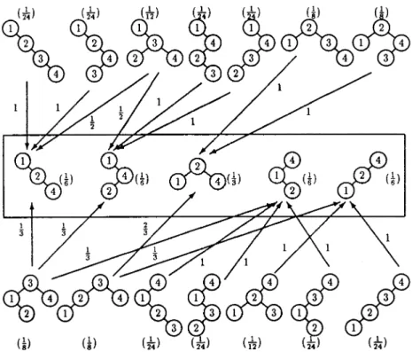
Figure 1 shows the effects of the insertion of x 5 3 in a random BST when

K 5 {1, 2, 4}. The probability that each BST has according to the random BST model appears enclosed in parentheses. The arrows indicate the possible out-comes of the insertion of x 5 3 in each tree and are labelled by the corresponding probabilities. This figure also gives us an example of Lemma 2.2. Consider only the arrows that end in trees whose root is 3. These arrows show the result of inserting at root the key 3 in a random BST for the set of keys {1, 2, 4}. Notice that the root of the left subtree is either 1 or 2 with the same probability. Hence, the tree containing the keys smaller than 3 in the original random BST is also a random BST for the set of keys {1, 2}.

As an immediate consequence of the Theorem 2.3, the next corollary follows:

COROLLARY 2.4. Let K5{x1, . . . ,xn}be any set of keys,where n$0.Let p5

xi1, . . . ,xinbe any fixed permutation of the keys in K.Then the RBST that we obtain after the insertion of the keys of p into an initially empty tree is a random binary search tree.More formally,if

T5insert~x_i_n, insert~x_i_n₂₁, . . . , insert~x_i₁, h!· · ·!!,

then T is a random BST for the set of keys K.

This corollary can be put into sharp contrast with the well-known fact that the standard insertion of a random permutation of a set of keys into an initially empty tree yields a random BST; the corollary states that for anyfixed permuta-tion we will get a random BST if we use the RBST inserpermuta-tion algorithm.

(8)

3. Deletions

The deletion algorithm uses a procedure calledjoin, which actually performs the

removal of the desired key (see Algorithm 3). To delete a key x from the given RBST, we first search forx, using the standard search algorithm until an external node orxis found. In the first case,x is not in the tree, so nothing must be done. In the second case, only the subtree whose root isx will be modified. Notice that most (if not all) deletion algorithms work so.

(9)

Let T be the subtree whose root is x. Let L and R denote the left and right subtrees of T, respectively, and K_,x and K.x denote the corresponding sets of

keys. To delete the node where x is located (the root ofT) we build a new BST

T9 5 join(L, R) containing the keys in the setK_,_xø K_._x and replaceT byT9.

By hypothesis, the join operation does only work when none of the keys in its

first argument is larger than any of the keys in its second argument.

Our definition of the result of joining two trees when one of them is empty is trivial:join(h,h)5 h,join(L, h) 5 L, and join(h, R) 5 R. Notice, however,

that Hibbard’s deletion algorithm does not follow all these equations.

Now, assume thatL andR are trees of sizem . 0 andn . 0, respectively. A common way to perform the join of two nonempty trees,L andR, is to look for the maximum key inL, sayz, delete it from L and let z be the common root of

L9 andR, whereL9 denotes the tree that results after the deletion of z fromL. Alternatively, we might take the minimum item in R and put it as the root of

join(L, R), using an analogous procedure. Deleting the maximum (minimum)

item in a BST is easy, since it cannot have a nonempty right (left) subtree. Our definition ofjoin, however, selects either the root ofL or the root ofR to

become the root of the resulting tree and then proceeds recursively. LetLl and

Lrdenote the left and right subtrees ofL and similarly, letRland Rrdenote the

subtrees ofR. Further, leta andb denote the roots of the treesL andR. As we already said, join chooses between a and b to become the root of T9 5 join(L,

R). Ifa is selected, then its left subtree isLl and its right subtree is the result of

joiningLr withR. Ifb were selected then we would keepRr as the right subtree

of T9 and obtain the left subtree by joining L with Rl. The probability that we

choose either aorb to be the root ofT9 ism/(m 1 n) foraand n/(m 1 n) for

b.

Just as the insertion algorithm of the previous section preserves randomness, the same happens with the deletion algorithm described above (Theorem 3.2). The preservation of randomness of our deletion algorithm stems from the corresponding property of join: the join of two random BSTs yields a random

BST. As we shall see soon, this follows from the choice of the probabilities for the selection of roots during the joining process.

LEMMA 3.1. Let L and R be two independent random BSTs,such that the keys

in L are strictly smaller than the keys in R.Let KLand KRdenote the sets of keys in

L and R,respectively.Then T5 join(L, R) is a random BST that contains the set

of keys K5 KLø KR.

PROOF. The lemma is proved by induction on the sizesm and n of L and R.

If m 5 0 or n 5 0, the lemma trivially holds, since join(L, R) returns the

nonempty tree in the pair, if there is any, andhif both are empty. Consider now the case where bothm . 0 andn . 0. Leta 5 L 3 keyandb 5 R 3 key. If

we selectato become the root ofT, then we will recursively joinLr5 L3 right

and R. By the inductive hypothesis, the result is a random BST. Therefore, we have that: (1) the left subtree of T is L 3 left and hence it is a random BST

(because so was L); (2) the right subtree of T is join(L_r, R), which is also

random; (3) both subtrees are independent; and (4) the probability that any key

x in L becomes the root of T is 1/(m 1 n), since this probability is just the probability thatx was the root ofL times the probability that it is selected as the

(10)

root ofT: 1/m 3 m/(m 1 n) 5 1/(m 1 n). The same reasoning shows that the lemma is also true ifb were selected to become the root ofT. e

THEOREM 3.2. If T is a random BST that contains the set of keys K, then

delete(x, T) produces a random BST containing the set of keys K\{x}.

PROOF. If x is not in T, then delete does not modify T and the theorem

trivially holds.

Let us suppose now thatx is in T. The theorem is proved by induction on the size n of T. If n 5 1, then delete(x, T) produces the empty tree, and the

theorem holds. Let us assume thatn . 1 and the theorem is true for all sizes,

n. Ifx was not the root ofT, then we deletex from the left or right subtree ofT

and, by induction, this subtree will be a random BST. Ifx was the root ofT, T9

5 delete(x, T) is the result of joining the left and right subtrees ofT, which by

last lemma will be a random BST. Therefore, both the left and right subtrees of

T9 are independent random BSTs. It is left to prove that every y [ K not equal to x has the same probability, 1/(n 2 1), of being the root of T9. This can be easily proved.

P@y is the root ofT9#5P@y is the root ofT9ux was the root ofT#

3P@x was the root ofT#

1P@y is the root ofT9ux was not the root of T#

3P@x was not the root of T#

5P@joinbringsy to the root ofT9#31/n

1P@y was the root ofTux was not the root ofT#

3~n21!/n 5 1 n213 1 n1 1 n213 n21 n 5 1 n21. e

(11)

Figure 2 shows the effects of the deletion ofx 5 3 from a random BST when

K 5 {1, 2, 3, 4}. The labels, arrows, etc. follow the same conventions as in Figure 1. Again, we can use this figure to give an example of the result of another operation, in this case join. Notice that the arrows that start in trees with root 3

show the result of joining two random BSTs, one with the set of keys KL 5 {1,

2} and the other with the set of keys K_R 5 {4}. The outcome is certainly a random BST with the set of keys {1, 2, 4}.

On the other hand, comparing Figures 1 and 2 produces this nice observation: For any fixed BST T, let P[T] be the probability of T according to the random BST model. Let T₁ and T₂ be any given BSTs with n and n 1 1 keys, respectively, and letx be any key not inT1. Then

P@T1#3P@Insertingx inT1produces T2#5

P@T2#3P@Deleting x fromT2 producesT1#.

Combining Theorem 2.3 and Theorem 3.2, we get this important corollary.

COROLLARY 3.3. The result of any arbitrary sequence of insertions and dele

-tions,starting from an initially empty tree,is always a random BST.Furthermore,if the insertions are random(not arbitrary),then the result is still a random BST even if the standard insertion algorithm or Stephenson’s insertion at root algorithm is used instead of the randomized insertion algorithm for RBSTs.

(12)

4. Performance Analysis

The analysis of the performance of the basic algorithms is immediate, since both insertions and deletions guarantee the randomness of their results. Therefore, the large collection of results about random BSTs found in the literature may be used here. We will use three well-known results2_{about random BSTs of size} _n_:

the expected depth of the ith internal node, the expected depth of the ith external node (leaf), and the total expected length of the right and left spinesof the subtree whose root is theith node. We will denote the corresponding random variables $n(i), +n(i), and 6n(i). Recall that the right spine of a tree is the path

from the root of the right son to the smallest element in that subtree. Analo-gously, the left spine is the path from the root of the left son to its largest element (see Figure 3). The expected values mentioned above are:

E@$n(i)#5Hi1Hn112i22, i51, . . . , n;

E@+n(i)#5Hi211Hn112i, i51, . . . , n11;

E@6n(i)#5E@+n(i)1+n(i11)22~$n(i)11!#522

1

i 2

1

n112i, i51, . . . , n;

where Hn 5 ¥i#j#n 1/j 5 ln n 1 g 1 2(1/n) denotes the nth harmonic

number, and g5 0.577 . . . is Euler’s constant.

To begin with, let Sn(i) and Un(i) be the number of comparisons in a successful

search for theith key and the number of comparisons in an unsuccessful search for a key in the ith interval of a tree of size n, respectively. It is clear that

2_{See, for example, Knuth [1973], Mahmoud [1992], Sedgewick and Flajolet [1996], and Vitter and} Flajolet [1990].

(13)

Sn(i)5$n(i)11, i51, . . . , n.

Un(i)5+n(i), i51, . . . , n11.

Let us consider now the cost of an insertion in theith interval (1 # i # n 1 1) of a tree of size n. If this cost is measured as the number of visited nodes, then its expected value is E[+n(i)] 1 1, since the visited nodes are the same as

those visited in an unsuccessful search that ends at theith external node, plus the new node. However, the insertion of a new item has two clearly differentiated phases and the cost of the stages differ in each of these two phases. Before the insertion at root, we generate a random number in each stage, compare it to another integer, and (except in the last step) compare the new key with the key at the current node. Notice that a top-down (nonrecursive) implementation of the insertion algorithm would not update the pointer to the current node, as Algorithm 1 does. In each stage of the insertion at root, a comparison between keys and updating of pointers take place, but no random number is generated.

Hence, for a more precise estimate of the cost of an insertion, we will divide this cost into two contributions: the cost of the descent until the new item reaches its final position, R_n(i)_{, plus the cost of restructuring the tree beneath,}

that is, the cost of the insertion at the root, I_n(i)_{. We measure these quantities as}

the number of steps or visited nodes in each. Consider the tree after the insertion. The number of nodes in the path from the root of the tree to the new item isR_n(i)_{. The nodes visited while performing the insertion at root are those in}

the left and the right spines of the subtree whose root is theith node. Since the tree produced by the insertion is random, we have

Rn(i)5$n(i)1111, I(i)n 56n(i)11, i51, . . . , n11.

As expected,E[Rn(i) 1 I(i)n ] 5 E[+n(i)] 1 1. A more precise estimation of the

expected cost of an insertion in the ith interval is then

aE@Rn(i)#1bE@In(i)#5a~Hi1Hn122i21!1b

S

22

1

i 2

1

n122i

D

,

whereaand bare constants that reflect the different costs of the stages in each of the two phases of the insertion algorithm. Notice that the expected cost of the insertion at root phase is2(1), since less than two rotation-like operations take place (on average).

The cost of the deletion, measured as the number of visited keys, of theith key of a tree of sizen is also easy to analyze. We can divide it into two contributions, as in the case of insertions: the cost of finding the key to be deleted, Fn(i), plus

the cost of the join phase, Jn(i). Since the input tree is random, we have

Fn(i)5$n(i)11, J(i)n 56n(i), i51, . . . , n.

Notice that the number of visited nodes while deleting a key is the same as while inserting it, because we visit the same nodes. The expected number of local updates per deletion is also less than two. A more precise estimation of the expected cost of the deletion of theith element is

(14)

a9~Hi1Hn112i21!1b9

S

22

1

i 2

1

n112i

D

,

wherea9andb9are constants that reflect the different costs of the stages in each of the two phases of the deletion algorithm. Altogether, the expected cost of any search (whether successful or not) and the expected cost of any update operation is alwaysU(logn).

The algorithms in the next section can also be analyzed in a straightforward manner. It suffices to relate their performance to the probabilistic behavior of well-known quantities like the depth of internal or external nodes in random BSTs, like we have done here.

5. Other Operations

5.1. DUPLICATE KEYS. In Section 2, we have assumed that whenever we

insert a new item in a RBST its key is not present in the tree. An obvious way to make sure that this is always the case is to perform a search of the key, and then insert it only if it were not present. But there is an important waste of time if this is naı¨vely implemented. There are several approaches to cope with the problem efficiently.

The bottom-up approach performs the search of the key first, until it either finds the sought item or reaches an external node. If the key is already present the algorithm does nothing else. If the search was unsuccessful, the external node is replaced with a new internal node containing the item. Then, zero or more single rotations are made, until the new item gets into its final position; the rotations are done as long as the random choices taken with the appropriate probabilities indicate so. This is just like running the insertion at root algorithm backwards: we have to stop rotations at the same point where we would have decided to perform an insertion at root. We leave the details of this kind of implementations as an exercise.

There is an equivalent recursive approach that uses a variant of split that does nothing (does not split) if it finds the key in the tree to be split. The sequence of recursive calls signal back such event and the insertion is not performed at the point where the random choice indicated so.

Yet there is another solution, using the top-down approach, which is more efficient than the other solutions considered before. We do the insertion almost in the usual way, with two variations:

(1) The insertion at root has to be modified to remove any duplicate of the key that we may find below (and we will surely find it when splitting the tree). This is easy to achieve with a slight modification of the procedure split;

(2) If we find the duplicate while performing the first stage of the insertion (i.e., when we are finding a place for the inserted key), we have to decide whether the key remains at the position where it has been found, or we push it down. The reason for the second variation is that, if we never pushed down a key which is repeatedly inserted, then this key would promote to the root and have more chances than other keys to become the root or nearby (see Subsection 5.3). The

(15)

modified insertion algorithm is exactly like Algorithm 1 given in Section 2, except that it now includes

if (x 55 T 3 key) return push_down(T);

after the comparison r 55 n has failed.

In order to push down an item, we basically insert it again, starting from its current position. The procedurepush_down(T) (see Algorithm 5) pushes down

the root of the treeT; in each step, we decide either to finish the process, or to push down the root to the left or to the right, mimicking single rotations. The procedurepush_down(T) satisfies the next theorem.

THEOREM 5.1.1. Let T be a BST such that its root is some known key x,and its

left and right subtrees are independent random BSTs. Then push_down(T)

pro-duces a completely random BST (without information on the root of the tree).

We shall not prove it here, but the result above allows us to generalize Theorem 2.3 to cope with the insertion of repeated keys.

THEOREM 5.1.2. If T is a random BST that contains the set of keys K and x is

any key(that may or may not belong to K),then insert(x, T) produces a random

BST containing the set of keys K ø {x}.

Although, for the sake of clarity, we have given here a recursive implementa-tion of theinsertion and push_downprocedures, it is straightforward to obtain

efficient iterative implementations of both procedures, with only additional constant auxiliary space (no stack) and without using pointer reversal.

(16)

5.2. SETOPERATIONS. We consider here three set operations: union,

intersec-tion, and difference.

Given two treesA andB, union(A,B) returns a BST that contains the keys in

A and B, deleting the duplicate keys. If both trees are empty, the result is also the empty tree. Otherwise, a root is selected from the roots of the two given trees, say, we select a5 A 3 key. Then, the tree whose root was not selected is

split with respect to the selected root. Following the example, we split B with respect to a, yielding B_, and B_.. Finally, we recursively perform the union of the left subtree of A with B_, and the union of the right subtree of A with B_.. The resulting unions are then attached to the common roota. If we selectb 5 B

3 keyto be the root of the resulting tree, then we check if b was already inA.

If this is the case, then b was duplicate and we push it down. Doing so we compensate for the fact thatbhas had twice the chances of being the root of the final tree as any nonduplicate key.

This algorithm uses a slight variant of the proceduresplit, which behaves like

the procedure described in Section 2, but also removes any duplicate of x, the given key, and returns 0 if such a duplicate has not been found, and 1 otherwise. The correctness of the algorithm is clear. A bit more involved proof shows that

union(A, B) is a random BST if bothA andB are random BSTs. The expected

cost of the unionis U(m 1 n), where m 5 A 3 size and n 5 B 3 size.

The intersection and set difference of two given treesA andB are computed in a similar vein. Algorithms 7 and 8 always produce a RBST, if the given trees are RBSTs. Notice that they do not need to use randomness. As in the case of the union of two given RBSTs, their expected performance is U(m 1 n). Both

intersectionand differenceuse a procedure free_tree(T), which returns all the

(17)

As a final remark, notice that for all our set algorithms we have assumed that their parameters had to be not only combined to produce the output, but

destroyed. It is easy to write slightly different versions that preserve their inputs. 5.3. SELF-ADJUSTINGSTRATEGIES. In Subsection 5.1, we have mentioned that

to cope with the problem of duplicate keys, we either make sure that the input tree is not modified at all if the new key is already present, or we add a mechanism to “push down” duplicate keys. The reason is that, if we did not have such a mechanism, a key that as repeatedly inserted would promote to the root. Such a key would be closer to the root with probability larger than the one corresponding to the random BST model, since that key would always be inserted at the same level that it already was or closer to the root.

This observation immediately suggests the following self-adjusting strategy: each time a key is searched for, the key is inserted again in the tree, but now it will not be pushed down if found during the search phase; we just stop the insertion. As a consequence, frequently accessed keys will get closer and closer to the root (because they are never inserted at a level below the level they were before the access), and the average cost per access will decrease.

We can rephrase the behavior of this self-adjusting strategy as follows: we go down the path from the root to the accessed item; at each node of this path we decide, with probability 1/n, whether we replace that node with the accessed item and rebuild the subtree rooted at the current node, or we continue one level below, unless we have reached the element we were searching for. Here, n

denotes the size of the subtree rooted at the current node. When we decide to replace some node by the sought element, the subtree is rebuilt and we should take care to remove the duplicate key.

Since it is not now our goal to maintain random BSTs, the probability of replacement can be totally arbitrary, not necessarily equal to 1/n. We can use any function 0 , a(n)# 1 as the probability of replacement. Ifa(n) is close to

(18)

1, then the self-adjusting strategy reacts quickly to the pattern of accesses. The limit case a(n) 5 1 is the well known move-to-root strategy [Allen and Munro 1978], because we always replace the root with the most recently accessed item and rebuild the tree in such a way that the result is the same as if we had moved the accessed item up to the root using single rotations. If a(n) is close to 0, convergence occurs at a slower rate, but it is more difficult to fool the heuristic with transient patterns. Obviously, the self-adjusting strategy that we have originally introduced is the one wherea(n) 5 1/n.

Notice that the different self-adjusting strategies that we consider here are just characterized by their corresponding functiona; no matter whata(n) is we have the following result, that will be proved in Section 7.

THEOREM 5.3.1. Let X 5 {x₁, . . . , x_N} and let T be a BST that contains the

items in X.Furthermore,consider a sequence of independent accesses to the items in X such that xi is accessed with probability pi. If we use any of the self-adjusting

strategies described above to modify T at each access, the asymptotic probability distribution is the same for all strategies and independent of a(n), namely, it is the one for the move-to-root strategy.

We know thus that after a large number of accesses have been made and the tree reorganized according to any of the heuristics described above, the proba-bility that xi is an ancestor of xj is, for i , j, pi/(pi 1 . . .1 pj). Moreover, the

average cost of a successful search is

C#N5112

O

1#i,j#N

pipj

pi1· · ·1pj

.

In the paper of Aragon and Seidel [1989], they describe another self-adjusting strategy for randomized treaps: each time an item is accessed, a new random

(19)

priority is computed for that item; if the new priority is larger than its previous priority, the older priority is replaced by the newer and the item is rotated upwards until heap order in the tree is restablished. This strategy does not correspond to any of the strategies in the family that we have discussed before, but it also satisfies Theorem 5.3.1. The analysis of the strategy suggested by Aragon and Seidel becomes simpler once we notice that its asymptotic distribu-tion is the same as that of move-to-root.

The main difference between the self-adjusting strategies that we have dis-cussed here is that they have different rates of convergence to the asymptotic distribution. Allen and Munro [1978] show that, for move-to-root, the difference between the average cost in the asymptotic distribution and the average cost aftert accesses is less than 1 ift $ (N logN)/e and the initial tree is random. If

a(n) , 1, it is clear that the rate of convergence should be slower than that for move-to-root. We have been able to prove that if a(n) is constant, then the result of Allen and Munro holds for t $ (N logN)/(a z e). We conjecture that this is also true for anya(n), but we have not been able to prove it. On the other hand, Aragon and Seidel did not address the question of the rate of convergence for their strategy and it seems also quite difficult to compute it.

In a more practical setting, the strategy of Aragon and Seidel has a serious drawback, since frequently accessed items get priorities close to 1. Then the length of the priorities tends to infinity as the number of accesses grows. The situation gets even worse if the p_i’s, the probabilities of access, changes from time to time, since their algorithms react very slowly after a great number of accesses have been made.

6. Implementation Issues

6.1. NUMBER OF RANDOM BITS. Let us now consider the complexity of our

algorithms from the point of view of the number of needed random bits per operation.

For insertions, a random number must be generated for each node visited before the placement of the new item at the root of some subtree is made. If the currently visited nodey is the root of a subtree of size m, we would generate a random number between 0 andm; if this random number ism, then we insert at root the new element; otherwise, the insertion continues either on the left or right subtree of y. If random numbers are generated from high-order to low-order bits and compared with prefixes of the binary representation of m, then the expected number of generated random bits per node is U(1)–most of the times the comparison fails and the insertion continues at the appropriate subtree. Recall that the expected number of nodes visited before we insert at root the new item is U(log n). The total expected number of random bits per insertion is thus U(log n). Further refinements could reduce the expected total number of random bits to U(1). Nevertheless, the reduction is achieved at the cost of performing rather complicated arithmetic operations for each visited node during the insertion.

In the case of deletions, the expected length of left and right spines of the node to be deleted is constant, so the expected number of random bits is also constant.

(20)

A practical implementation, though, will use the straightforward approach. Typical random number generators produce one random word (say of 32 or 64 bits) quite efficiently and that is enough for most ordinary applications.

6.2. NON-RECURSIVE TOP-DOWN IMPLEMENTATION OF THE OPERATIONS. We

have given recursive implementations of the insertion and deletion algorithms, as well as for other related procedures. It is not very difficult to obtain efficient nonrecursive implementations of all considered operations, with two interesting features: they only use a constant amount of auxiliary space and they work in pure top-down fashion. Thus, these nonrecursive implementations do not use stacks or pointer reversal, and never traverse a search path backwards. We also introduce an apparently new technique to manage subtree sizes without modify-ing the top-down nature of our algorithms (see next subsection for more details). As an example, Algorithm 10 in Appendix A shows a nonrecursive implementa-tion of the deleimplementa-tion algorithm, including the code to manage subtree sizes.

6.3. MANAGEMENT OF SUBTREE SIZES AND SPACE COMPLEXITY. Up to now,

we have not considered the problem of managing the sizes of subtrees. In principle, each node of the tree has to store information from which we can compute the size of the subtree rooted at that particular node. If the size of each subtree is stored at its root, then we face the problem of updating this information for all nodes in the path followed during insertion and deletion operations. The problem gets more complicated if one has to cope with insertions that may not increase the size of the tree (when the element was already in the tree) and deletions that may not decrease the size (when the element to be deleted was not in the tree).

A good solution to this problem is to store at each node the size of its left son or its right son, rather than the size of the subtree rooted at that node. An additionalorientation bit indicates whether the size is that of the left or the right subtree. If the total size of the tree is known and we follow any path from the root downwards, it is easy to see that, for each node in this path, we can trivially compute the sizes of its two subtrees, given the size of one of them and its total size. This trick notably simplifies the management of the size information: for instance, while doing an insertion or deletion, we change the size and orientation bit of the node from left to right if the operation continues in the left subtree and the orientation bit was ‘left’; we change from right to left in the symmetric case. When the insertion or deletion finishes, only the global counter of the size of the tree has to be changed if necessary (see Algorithm 10 in Appendix A). Similar rules can be used for the implementation of splits and joins.

We emphasize again that the information about subtree sizes – required by all our algorithms – can be advantageously used for operations based on ranks, like searching or deleting theith item. In fact, since we store either the size of the left or the right subtree of each node, rank operations are easier and more efficient. By contrast, if the size of the subtree were stored at the node, one level of indirection (examining the left subtree root’s size, for instance) would be necessary to decide if the rank operation had to continue either to the left or to the right.

Last but not least, storing the sizes of subtrees is not too demanding. The expected total number of bits that are necessary to store the sizes is U(n) (this

(21)

result is the solution of the corresponding easy divide-and-conquer recurrence). This is well below theU(n log n) number of bits needed for pointers and keys. 7. Formal Framework and Algebraic Proofs

7.1. RANDOMIZEDALGORITHMS. Although the behavior of deterministic

algo-rithms can be neatly described by means of algebraic equations, this approach has never been used for the study of randomized algorithms in previous works. We now present an algebraic-like notation that allows a concise and rigorous description and further reasoning about randomized algorithms, following the ideas introduced in Martı´nez and Messeguer [1990].

The main idea is to consider any randomized algorithmF as a function from the set of inputs A to the set ofprobability functions(or PFs, for short) over the set of outputs B. We say thatf is a probability function overB if and only iff: B

3 [0, 1] and ¥_y_[_B _f₍_y₎ ₅ _{1, as usual.}

Letf1, . . . ,fnbe PFs overB and leta1, . . . , an [ [0, 1] be such that¥1#i#n

ai 5 1. Consider the following process:

(1) Choose some PF from the set {fi}i51, . . . , n in such a way that eachfi has a

probabilityai of being selected.

(2) Choose one element from B according to the probabilities defined by the selected fi, namely, choosey [ B with probability fi(y).

Leth be the PF over B related to the process above: for anyy [ B, h(y) is the probability that we select the element y as the outcome of the whole process. Clearly,h is the linear combinationof thefi’s with coefficientsai’s:

h5a1zf11· · ·1anzfn5

O

1#i#n

aizfi. (2)

The linear combination of PFs modelizes the common situation where a random-ized algorithm h makes a random choice and depending on it performs some particular task fi with probabilityai.

Let f be a PF over Bsuch thatf(b) 5 1 for someb [ B (i.e.,f(y)5 0 for all

y Þ b). Then, we will writef 5 b. Thus, we are considering each element inBas a PF overB itself:

b~y!5

H

1,_0, if_otherwise.y5b, (3) This convention is useful, since it will allow us to uniformly deal with both randomized and deterministic algorithms.

Letf be any PF overB 5 {yi}i, and letpi denotef(yi). Then, the convention

above allows us to writef 5 ¥_i _p_i _z _y_i_{, since for any}_y_j _[ _B_{, we have that} _f₍_y_j₎

5 [¥_i _p_i _z _y_i_](_y_j₎ ₅ ¥_i _p_i _z _y_i₍_y_j₎ ₅ _p_j_{. Taking into account that} _p_i ₅ _f₍_y_i_{), we}

get the following equality, that may look amazing at first:

f5

O

y[B

(22)

LetF be a randomized algorithm from the input setA to the output setB. Fix some inputx [ A. We denote byF(x) the PF over B such that, for any y [ B, [F(x)](y) is the probability that the algorithm F outputsy when given input x. Let {y1, . . . , ym} be the set of possible outputs of F, whenx is the input given

to F, and let pi be the probability that yi is the actual output. Then, using the

notation previously introduced, we may write

F~x!5p1zy11· · ·1pmzym. (5)

Notice that, if for somea [ A the result ofF(a) is always a fixed elementb [

B, then the expression above reduces to F(a) 5 b.

Finally, we characterize the behavior of the sequential composition of random-ized algorithms. Letg be a PF over A, and letF be a function from A to B. By

F(g), we will denote the PF overB such that [F(g)](y) is the probability that y

is the output of algorithm F when the input is selected according to g. It turns out thatF(g) is easily computed from g and the PFs F(x) for each elementx in

A. F~g!5F

S

O

x[A g~x!zx

D

5

O

x[A g~x!zF~x!. (6)

Recall that a single element a from A may be considered as a PF over A, and then the definition above is consistent with the case g 5 a, that is, when the input of F is fixed, since ¥_x_[_A _a₍_x₎ _z _F₍_x₎ ₅ _F₍_a_).

We shall also use Iverson’s bracket convention for predicates, that is,vPb is 1 if the predicateP is true, and 0, otherwise. This convention allows expressing the definitions by cases as linear combinations.

7.2. BINARY SEARCH TREES AND PERMUTATIONS. We now introduce some

definitions and notation concerning the main types of objects we are coping with: keys, permutations and trees.

Given a finite set of keys K, we shall denote @(K) the set of all BSTs that contain all the keys inK. For simplicity, we will assume thatK , N. The empty tree is denoted byh. We will sometimes omit drawing empty subtrees, to make the figures simpler. A tree T with root x, left subtree L and right subtreeR is depicted T5

V

x

/ \

L R .

Similarly, we denote 3(K) the set of all permutations (sequences without repetition) of the keys in K. We shall use the terms sequence and permutation with the same meaning for the rest of this paper. The empty sequence is denoted bylandUuVdenotes the concatenation of the sequencesUandV(provided that

U and V do not have common elements).

The following equations relate sequences in3(K) and BSTs in@(K). Given a sequenceS, bst(S) is the BST resulting after the standard insertion of the keys

(23)

bst~l!5h, bst~xuS!5

V

x

}

{

bst~sep,~x, S!! bst~sep.~x, S!!

, (7)

where the algebraic functionsep_,(x,S) returns the subsequence of elements in

S smaller than x, and sep_.(x, S) returns the subsequence of elements in S

larger than x. Both functions respect the order in which the keys appear in S.

Let Random_Perm be a function such that, given a set K with n $ 0 keys,

returns a randomly chosen permutation of the keys in K. It can be compactly written as follows:

Random Perm~K!5

O

P[3(K)

1

n!zP. (8)

Random BSTs can be defined in the following succint way, which turns out to be equivalent to the assumption that a RBST of sizen is built by performing n

random insertions in an initially empty tree:

RBST~K!5bst~Random_Perm~K!!5

O

x[K 1 n.

V

x

} {

RBST~K_,_x! RBST(K_.x) . (9)

The last expression in the equation above is clearly equivalent to the one we gave in Section 2, provided we define its value to beh if n 5 0.

For instance, RBST~$1, 5, 7%!5bst~Random_Perm~$1, 5, 7%!! 5bst

S

1 6z1571 1 6z175 1 1 6z5171 1 6z5711 1 6z7151 1 6z751

D

We introduce now three useful algebraic functions over sequences:rm, shuffle

and equiv. The first function removes a key x from a sequence S [ 3(K), if

present, without changing the relative order of the other keys. For instance,

rm(3, 2315)5 215,rm(4, 2315)5 2315.

The function shuffleproduces a random shuffling of two given sequences with

no common elements. Let K₁ and K₂ be two disjoint sets with m and n keys, respectively. LetU 5 u1u . . .u um [ 3(K1) andV5 v1u . . .u vn [ 3(K2). We

define 6(U, V) as the set of all the permutations of the keys in K1 ø K2 that

could be obtained by shufflingU and V, without changing the relative order of the keys of U and V. Hence, 6(U, V) is the set of all Y 5 y₁ u . . .u y_m₁_n [

3(K1 ø K2) such that if yi 5 uj and y9i 5 u9j, then i , i9 if and only if j , j9

(and the equivalent condition for the keys of V). For instance, 6(21, ba) 5 {21ba, 2b1a, 2ba1, b21a, b2a1, ba21}. The number of elements in 6(U, V) is clearly equal to (mm1n). Therefore, we can rigorously define shuffle as a

function that, given U and V, returns a randomly choosen element from 6(U,

V). For instance, shuffle(21, ba) 5 1/6 z 21ba 1 1/6 z 2b1a 1 1/6 z 2ba1 1

1/6 z b21a 1 1/6 z b2a1 1 1/6 z ba21. The algebraic equations for shuffle are

shuffle~l, l!5l, shuffle~l, vuV!5vuV, shuffle~uuU, l!5uuU,

shuffle~uuU, vuV!5 m

m1nzuushuffle~U, vuV!1

n

m1nzvushuffle~uuU, V!,

(10) wherem andn are the sizes of uuU and ofvuV, respectively. It is not difficult to prove by induction that this definition of the functionshuffle is correct.

LetK be a set of keys and x a key not in K. We can use shuffle to define the

functionRandom_Permin the following inductive way, equivalent to definition (8):

Random Perm(À)5l,

Random Perm~Kø$x%!5shuffle~x, Random Perm~K!!. (11)

We defineequiv as a function such that given input a sequenceS [ 3(K), it

returns a randomly chosen element from the set of sequences that produce the same BST asS, that is,

%~S!5$E[3~K!ubst~E!5bst~S!%.

For example,%(3124)5{3124, 3142, 3412} andequiv(3124)51/3z312411/3z

3142 1 1/3 z 3412, since bst(3124) 5 bst(3142) 5 bst(3412) and no other

permutation of the keys {1, 2, 3, 4} produces the same tree. Using the function

shuffle, the equational definition ofequiv is almost trivial:

equiv~l!5l, (12)

equiv~xuS!5xushuffle~equiv~sep_,~x, S!!, equiv~sep_.~x, S!!!.

7.3. THE ALGORITHMS. In this subsection, we give equational definitions for

y

} {

L insert~x, R!

2

,

(25)

assuming that we never insert a key that was already in the tree. The functioninsert_at_rootcan be defined as follows:

insert_at_root~x, T!5

V

x

}

{

split,~x, T! split.~x, T!

, (14)

wheresplit_,andsplit_.are functions that, given a treeT and a keyx¸ T, return

a BST with the keys inT less thanx and a BST with the keys inT greater than x, respectively. The algebraic equations for the functionsplit_, are

split_,~x, h!5h, split_,

1

L delete~x,R! (16) 1[[x5y]]zjoin~L, R!.

The probabilistic behavior ofjoin can in turn be described as follows, when at

least one of its arguments is an empty tree:

join(h,h)5h, join~L, h!5L, join~h, R!5R.

On the other hand, when both arguments are non-empty trees, with sizesm 5 L

3 size . 0 andn 5 R 3 size. 0, respectively, we have

join~L, R!5 m m1nz

V

a

} {

Ll join~Lr, R! 1 n m1nz

V

b

} {

join~L, R_l! R_r , (17) wherea 5 L 3 key, L_l 5 L 3 left, L_r 5 L 3 rightand b 5 R 3 key, R_l 5

R 3 left, R_r 5 R 3 right.

7.4. THE PROOFS. We consider here several of the results that we have

already seen in previous sections as well as some intermediate lemmas that are interesting on their own. We will not provide proofs for all them, for the sake of brevity. Only the proof of Lemma 7.4.3 and Theorem 7.4.4 will be rather

(26)

detailed; in other cases, the proofs will be sketchy or just missing. However, the ones given here should suffice to exemplify the basic manuvers that the algebraic notation allows and typical reasoning using it.

The following lemma describes the result ofsplitwhen applied to a fixed BST.

LEMMA 7.4.1. Let S be any permutation of keys and let x be any key not in S.

Then

split~x, bst~S!!5@bst~sep_,~x, S!!,bst~sep_.~x, S!!#.

From this lemma, we can describe the behavior of split when applied to a random BST. Our next theorem is nothing but Lemma 2.2, now in the formal setting of this section.

THEOREM 7.4.2. Let K be any set of keys and let x be any key not in K.Let K_,x

and K_.xdenote the set with the keys in K less than x and the set with the keys in K

greater than x,respectively.Then

split~x, RBST~K!!5@RBST~K_,_x!, RBST~K_._x!#.

Lemma 7.4.1 relates split with sep, the analogous function over sequences.

Our next objective is to relate insert withshuffleandequiv, the functions that we

have defined before. The idea is that the insertion of a new item in a tree T has the same effect as taking at random any of the sequences that would produceT, placing x anywhere in the chosen sequence (an insertion-like operation in a sequence) and then rebuilding the tree. This is formally stated in the next lemma. LEMMA 7.4.3. Let S be any permutation of keys and let x be any key not in S.

Then

insert~x, bst~S!!5bst~shuffle~x, equiv~S!!!.

For instance, using Eqs. (7), (13), (14), and (15), we get

On the other hand, by the definitions of shuffle and equiv (Eqs. (10) and

(12)),

bst~shuffle~3, equiv~241!!!5bst

S

shuffle

S

3,1

which gives the same result asinsert(3, bst(241)), since the sequences in {3241,

3214} produce the first tree, those in {2341, 2314, 2134} produce the second tree, and the ones in {2431, 2413, 2143} produce the third.

PROOF. We prove the lemma by induction on n, the length ofS. Ifn 5 0,

insert~x, bst~l!!5insert~x, h!5

V

x

/ \

h h

,

but on the other hand,equiv(l)5landshuffle(x,l)5 x, so the lemma is true.

Assume now that n . 0, S 5 yuP and x is not present inS. Moreover, let us assume that x , y (the case x . y is very similar).

First of all, notice that, ifyuQis any permutation ofn keys andx is any key not inyuQ, then shuffle@x, yuQ#5 1 n11zxuyuQ1 n n11zyushuffle@x, Q#. Therefore, shuffle@x, equiv~yuP!#

$by definition ofequiv%

5shuffle@x, yushuffle@equiv~sep,~y, P!!, equiv~sep.~y, P!!##

$by the observation above%

5 1

n11zxuyushuffle@equiv~sep,~y, P!!, equiv~sep.~y, P!!#

1 n

n11zyushuffle@x, shuffle@equiv~sep,~y, P!!,

equiv~sep_.~y, P!!]].

Now we can use the definition ofequiv back in the first line. Furthermore, the

shuffleoperation is associative – we do not prove it, but it is easy to do it and

rather intuitive. Therefore,

shuffle@x, equiv~yuP!#5 1

n11zxuequiv~yuP!

1 n

n11zyushuffle@shuffle@x, equiv~sep,~y, P!!#,

equiv~sep_.~y, P!!].