Estimation For Image Denoising
Rajesh Kumar Gupta
Department of Computer Science and Engineering
National Institute of Technology Rourkela
Estimation For Image Denoising
Dissertation submitted inMay 2014 to the department of
Computer Science and Engineering
of
National Institute of Technology Rourkela
in partial fulfillment of the requirements for the degree of
Master of Technology
by
Rajesh Kumar Gupta
(Roll 212CS1090) under the supervision of
Dr. Ratnakar Dash
Department of Computer Science and Engineering National Institute of Technology Rourkela
National Institute of Technology Rourkela
Rourkela-769 008, India.
www.nitrkl.ac.inMay , 2014
Certificate
This is to certify that the work in the thesis entitled Multiscale LMMSE Based Statistical Estimation For Image Denoising byRajesh Kumar Gupta, bearing roll number 212CS1090, is a record of research work carried out by him under my supervision and guidance in partial fulfillment of the requirements for the award of the degree of Master of Technology inComputer Science and Engineering.
Dr. Ratnakar Dash Assistant Professor CSE Department
I, Rajesh Kumar Gupta (Roll No. 212CS1090) understand that plagiarism is defined as any one or the combination of the following
1. Uncredited verbatim copying of individual sentences, paragraphs or illustrations (such as graphs, diagrams, etc.) from any source, published or unpublished, including the internet.
2. Uncredited improper paraphrasing of pages or paragraphs (changing a few words or phrases, or rearranging the original sentence order).
3. Credited verbatim copying of a major portion of a paper (or thesis chapter) without clear delineation of who did or wrote what. (Source: IEEE, the Institute, Dec. 2004)
I have made sure that all the ideas, expressions, graphs, diagrams, etc., that are not a result of my work, are properly credited. Long phrases or sentences that had to be used verbatim from published literature have been clearly identified using quotation marks.
I affirm that no portion of my work can be considered as plagiarism and I take full responsibility if such a complaint occurs. I understand fully well that the guide of the thesis may not be in a position to check for the possibility of such incidences of plagiarism in this body of work.
Rajesh Kumar Gupta Roll: 212CS1090 Department of Computer Science
This dissertation, though an individual work, has benefited in various ways from several people. Whilst it would be simple to name them all, it would not be easy to thank them enough.
The enthusiastic guidance and support of Asst. Prof. Ratnakar Dash inspired me to stretch beyond my limits. His profound insight has guided my thinking to improve the final product. My solemnest gratefulness to him.
I am also grateful to Prof. Banshidhar Majhi for his ceaseless support throughout my research work.
It is indeed a privilege to be associated with people like Prof. S. K. Rath, Prof. S.K.Jena, Prof. D. P. Mohapatra, Prof. A. K. Turuk, Prof. S.Chinara, Prof. Pankaj Sa and Prof. B. D. Sahoo. They have made available their support in a number of ways.
Many thanks to my comrades and fellow research colleagues. It gives me a sense of happiness to be with you all. Special thanks to Anshuman,Anoop, Priyesh, Manish, Vijay and Vipul whose support gave a new breath to my research.
Finally, my heartfelt thanks for her unconditional love and support. Words fail me to express my gratitude to my beloved parents who sacrificed their comfort for my betterment.
Image Denoising is the process of removal of the noise from the image contaminated by additive Gaussian noise without loss of features of image. It is a fundamental process in pattern recognition and image processing.In this thesis,a wavelet based new denoising scheme for estimation of parameters such as variance of the multiscale Linear minimum mean square error(LMMSE) estimator to derive optimal threshold using maximum a posterior (MAP) estimator of the noisy coefficients in wavelet domain has been proposed. Our proposed scheme modify the parameter of LMMSE. Input image is decomposed in four wavelet subband then for each subband the LMMSE estimator is then applied.Denoised image is reconstructed after applying inverse wavelet transform. Each schemes is studied separately and experiments are conducted on test images to evaluate the performance.This denoising scheme shows the best performance for highly corrupted image in terms of the structure similarity index measure(SSIM)the peak signal-to-noise ratio (PSNR).
Keywords: Discrete Wavelet Transform, additive Gaussian noise, maximum a
Certificate ii
Declaration iii
Acknowledgment iv
Abstract v
List of Figures viii
List of Tables x
1 Introduction 1
1.0.1 What is image denoising? . . . 1
1.0.2 Why is denoising important? . . . 1
1.0.3 Problem Formulation . . . 2
1.0.4 Image Denoising versus Image Enhancement . . . 3
1.0.5 Noise model . . . 3
1.0.6 Introduction to the Wavelet Transform in Image Denoising . 4 1.0.7 Computing 2-D DWT and IDWT through subband analysis and synthesis . . . 5
1.1 Performance Measurement . . . 8
1.1.1 PSNR comparison . . . 8
1.1.2 SSIM comparison [30] . . . 8
2 Literature Review 11
2.1 Image denoising Techniques . . . 11
2.2 Wavelet Thresholding methods . . . 11
2.3 Denoising using Neighboring Coefficients [17] . . . 12
2.4 A generalized wavelet based denoising technique using neighboring wavelet coefficients [10] . . . 13
2.5 An improved adaptive wavelet based denoising technique using neighboring wavelet coefficients [22] . . . 13
2.6 Bivariate Shrinkage scheme for image denoising [11] . . . 14
2.7 LMMSE-Based Image Denoising [7] . . . 15
2.8 MAP Estimation based image denoising Using the BKF Prior [14] . 15 2.9 Image denoising using support vector machine(SVM) [15] . . . 16
3 Multiscale LMMSE Based Statistical Estimations 17 3.1 Statistical model . . . 18
3.1.1 LMMSE of Wavelet Coefficients . . . 18
3.1.2 MAP and ML estimations . . . 19
3.2 Denoising Algorithm . . . 22
3.3 Parameter Estimation . . . 22
3.4 Experiment and Results . . . 23
4 Conclusions and Future Scope 39 4.1 Conclusion . . . 39
4.2 Future Scope . . . 40
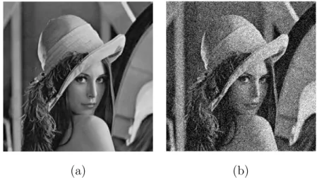
1.1 (a) Original Lena image. (b) Noisy Lena image . . . 2 1.2 (a) Original Image(b) wavelet coefficient at horizontal ,vertical and
diagonal direction. . . 6 1.3 (a) One stage decomposition of the 2-D Wavelet Transform,wavelet
coefficient at horizontal ,vertical and diagonal direction.(b) Inverse 2-D Wavelet Transform of wavelet. coefficient . . . 7
3.1 Illustrated Diagram of proposed method. . . 18 3.2 Neighborhood window selection . . . 21 3.3 Four 256×256 test images taken for experiment purpose(a) Lena.(b)
House.(c) Barbara.(d) Cameraman. . . 24 3.4 (a) Noisy Lena with (σ = 20) (b) Denoised using neighshrink
(28.56db) (c)Denoised using Bivariate (30.50db) (d) Denoised using GIDNWC (29.22db) (e)Denoised using IAWDMBNC (29.56db) (f)Denoised Image using MLMMSE (30.74db) . . . 25 3.5 (a)Cameraman Image with noise level (σ = 20) (b) Denoised
using neighshrink (26.44db) (c)Denoised using Bivariate (30.23db) (d) Denoised using GIDNWC (27.42db) (e)Denoised using IAWDMBNC (27.76db) (f)Denoised using MLMMSE (30.40db) . . . 26 3.6 Denoised Lena images(a) Noisy Lena Image (σ = 10) (c) Noisy
Lena Image (σ = 20) (e) Noisy Lena Image (σ = 30) (b),(d),(f) Denoised Images by Proposed Method. . . 27 3.7 Denoised Lena images (a) Noisy Lena Image (σ = 50) (c) Noisy
(σ= 30) (b),(d),(f) Denoised Images by Proposed Method. . . 29
3.9 Denoised Cameraman images (a) Noisy Cameraman Image (σ = 50) (c) Noisy Cameraman Image (σ= 100) (b),(d) Denoised Images by Proposed Method. . . 30
3.10 Denoised House images (a) Noisy House Image (σ = 10) (c) Noisy House Image (σ = 20) (e) Noisy House Image (σ = 30) (b),(d),(f) Denoised Images by Proposed Method. . . 31
3.11 Denoised House images (a) Noisy House Image (σ = 50) (c) Noisy House Image (σ= 100) (b),(d) Denoised Images by Proposed Method. 32 3.12 Denoised Barbara images (a) Noisy Barbaran Image (σ = 10) (c) Noisy Barbara Image (σ = 20) (e) Noisy Barbaran Image (σ = 30) (b),(d),(f) Denoised Images by Proposed Method. . . 33
3.13 Denoised Barbara images (a) Noisy Barbara Image (σ = 50) (c) Noisy Barbara Image (σ = 100) (b),(d) Denoised Images by Proposed Method. . . 34
3.14 Denoising performance comparison of Lena image . . . 37
3.15 Denoising performance comparison of Barbara image . . . 37
3.16 Denoising performance comparison of Cameraman image . . . 38
3.1 PSNR(dB) Image Denoising Performance Table For Lena, Cameraman, Barbara, and house images . . . 35 3.2 SSIM Image Denoising Performance Table ForLena,Cameraman,
Introduction
The objective of this chapter is to define the problem of image denoising and describes about the condition in which image denoising is important. Also discuss about performance measures to evaluate image denoising results.
1.0.1
What is image denoising?
Image denoising is the problem of restoring a clean image from a noisy image [1]. In most cases, it is assumed that the noisy or corrupted image is the summation of original image and a noise component,as shown in Figure 1.1. Hence denoising is a procedure which removes the existing noise in an image and minimizes the loss of features in a clean image. It involves prior knowledge: One knows something about images and about the noise. Without prior knowledge, image denoising would be impossible.
1.0.2
Why is denoising important?
Image Denoising is the part of preprocessing in Pattern Recognition system.The digital images sensed by sensors are generally corrupted by Gaussian noise during the process of acquisition, transmission, and retrieval from storage media. During the image acquisition process and interference noise may be generated due to improper settings of sensors used in image processing. A noisy image is not
pleasant to view.Therefore, it is very important to get the improved image from the corrupted image without loss of features of the image. In Pattern recognition it need a denoised image to work effectively. Random and uncorrelated noise samples are not compressible.So the motivation behind the denoising algorithm is to remove Gaussian noise. So all these factor give importance of denoising in image processing.
1.0.3
Problem Formulation
The problem of denoising can be mathematically presented as follows,
Y =X+η (1.1)
Let X be a original image with size N ×N, Y be a observed noisy image and η be zero-mean Gaussian noise with variance σ2,whereη ∈N(0, σ2)
The objective is to estimate true image X from given noisy image Y. A best estimate can be written as the conditional mean ˆX =E[X|Y] The difficulty lies in determining the probability density functionρ(x|y) here,the goal is to estimate the true image X from the noisy image Y without loss of features of the original image.
(a) (b)
1.0.4
Image Denoising versus Image Enhancement
Image denoising is different from image enhancement. As Gonzalez and Woods [1] explain, image enhancement is an objective process, whereas image denoising is a subjective process. Image denoising is the problem of restoring a clean image from a noisy that has been corrupted by using prior knowledge of the degradation process. Image enhancement, on the other hand, involves manipulation of the image characteristics to make it more appealing to the human eye. There is some overlap between the two processes.
1.0.5
Noise model
As Gonzalez and Woods [1] explain, A lens focuses the light from regions of interest onto a sensor. The sensor measures the color and light intensity. An analog-to-digital converter (ADC) converts the image to the digital signal. An Image processing block enhances the image and compensates for some of the deficiencies of the other camera blocks. Memory is present to store the image, while a display may be used to preview it. Some blocks exist for the purpose of user control. Noise is added to the image in the lens, sensor, and ADC as well as in the image processing block itself.
The sensor is made of millions of tiny light-sensitive components [1]. They differ in their physical, electrical, and optical properties, which adds a signal-independent noise (termed as dark current shot noise) to the acquired image. Another component of shot noise is the photon shot noise. This occurs because the number of photons detected varies across different parts of the sensor. Amplification of sensor signals adds amplification noise, which is zero mean Gaussian noise. There are many other types of noise exist. Correlated noise with a Guassian distribution is an example. Noise can also have different distributions such as Poisson, Laplacian, or non-additive Salt-and-Pepper noise. It is caused by bit errors in image transmission and retrieval as well as in analog-to-digital converters. A scratch in a picture is also a type of noise. Noise can be signal dependent or signal independent. For example, the process of quantization
(dividing a continuous signal into discrete levels) [1]. It is also focused on zero mean additive Gaussian noise due to its simple nature and generic. For correlated noise with a non-zero mean, the zero mean model can be derived by subtracting the mean after de-correlating the samples.
Gaussian noise [1] is the type of statistical noise which have probability density function same as the normal distribution,given by:
pG(z) = 1 σ√2πexp
−(z−µ)2
/2σ2
(1.2)
whereσ the standard deviation,µthe mean value and z represents the gray level.
1.0.6
Introduction to the Wavelet Transform in Image
Denoising
The wavelet transform is a efficient tool used in image denoising [1]. The main task in denoising is to estimate the true image from the corrupted image by differentiating it from the signal. Advantages of wavelet transform are as follows:
• Energy compactness refers that most of the signal energy is contained in a few large wavelet coefficients, but a small portion of the energy is spread across a large number of small wavelet coefficients. These coefficients represent details as well as high frequency noise in the image. By appropriately thresholding these wavelet coefficients, image denoising is achieved while preserving fine structures in the image.
• Blocking artifacts are not produced in WT but DCT produces.
• Wavelets allow multi-resolution analysis at different scales or resolution.It permits us to describe an image in terms of frequency at a position in the image [1].
Donoho [5] shows that wavelets are near optimal for compression, denoising, and detection of a wide class of signals. Wavelets are discretely sampled in discrete wavelet transform (DWT).It captures both frequency and location information so
temporal resolution is key advantage it has over Fourier transforms. A wave is usually defined as an oscillating function in time or space. Sinusoids are an example. Fourier analysis is a wave analysis. A wavelet is defined as a small wave that has its energy concentrated in time and frequency.It allows simultaneous time and frequency analysis with a flexible mathematical foundation while retaining the oscillating wave-like characteristic.It provides a tool for the analysis of time-varying,non-stationary, and transient phenomena. Instead of considering a continuous signal, if we consider a discrete sequence s(n), defined for n = 0,1,2,3... the resulting coefficients in the series expansion are called the Discrete Wavelet Transforms (DWT) of s(n). The coefficients of series expansions shown in equations (1.3) and (1.4) for discrete signal to obtain the DWT coefficients, given by Wφ(j0, k) = 1 √ M X n s(n)φj0,k(n) (1.3) Wψ(j, k) = √1 M X n s(n)ψj,k(n) (1.4)
where,j ≥ j0 and s(n), φj0,k(n) and ψj,k(n) are functions of discrete variables
n = 0,1,2...M−1. Equation (1.3) computes the approximation coefficients and equation (1.4) computes the detail coefficients. The corresponding Inverse Discrete Wavelet Transform (IDWT) to express the discrete signal in terms of the wavelet coefficients can be written as
s(n) = √1 M X k Wφ(j0, k)φj0,k(n) + ∞ X j=0 X k Wφ(j, k)ψj,k(n) (1.5)
Normally, we let j0 = 0 and select M to be a power of 2(M = 2j) so that the
summations are performed over j=0,1,2...J-1 and k=0,1,2...2j−1.
1.0.7
Computing 2-D DWT and IDWT through subband
analysis and synthesis
The concepts of one-dimensional DWT [1] and its implementation through subband coding can be easily extended to two-dimensional signals for digital
(a) (b)
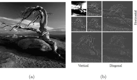
Figure 1.2: (a) Original Image(b) wavelet coefficient at horizontal ,vertical and diagonal direction.
images. In case of subband analysis of images, DWT perform two dimensional wavelet decomposition. It compute approximation coefficient, and detail coefficients in horizontal, vertical, diagonal directions. The analysis of 2-D wavelet signals require the use of 2-D filter functions through the product of separable wavelet and scaling functions in n2(vertical) and n1(horizontal) directions :
φ(n1, n2) =φ(n1)φ(n2) (1.6)
ψH(n1, n2) =ψ(n1)φ(n2) (1.7)
ψV(n1, n2) =φ(n1)ψ(n2) (1.8)
ψD(n1, n2) =ψ(n1)ψ(n2) (1.9)
In the above equations ψD(n
1, n2, ψV(n1, n2), ψH(n1, n2), φ(n1, n2)) represent the
signals with diagonal details, vertical details, horizontal details, and approximated signal respectively.
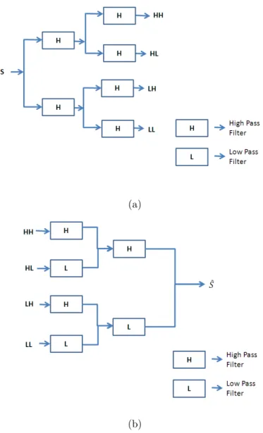
In subband coding the low-pass (L) and high-pass (H) filters along the columns (vertical direction) and along the rows (horizontal direction) are used . The bands ψD(n
1, n2, ψV(n1, n2), ψH(n1, n2), φ(n1, n2)) are also referred to as HH, HL, LH,
(a)
(b)
Figure 1.3: (a) One stage decomposition of the 2-D Wavelet Transform,wavelet coefficient at horizontal ,vertical and diagonal direction.(b) Inverse 2-D Wavelet Transform of wavelet. coefficient
1.1
Performance Measurement
Images are corrupted with Gaussian noise and then denoised using various methods.The random noise added to the image with the different standard deviation. Performance of wavelet based denoising algorithm is measured in terms of following two method:
1.1.1
PSNR comparison
Peak signal to noise ratio(PSNR) is used as quality measurement in decibels between original and noisy image.
To compute PSNR the block first calculate Mean Square Error(MSE) using the following Formula:
MSE = X I,J (A1(i, j)−A2(i, j))2 I×J (1.10) PSNR = 10 log10 r 2 MSE (1.11)
where I×J is the size of the image and r is the most extreme variance in the image data type.
1.1.2
SSIM comparison [30]
Structural similarity(SSIM) index is a technique for measuring the similarity of structural information between two input images. It is a fully reference metric i.e it measure the quality of image based on original noise-free image as reference. [30]. The SSIM metric is measured between two windows p and q of common size M ×M is
SSIM(p, q) = (2µpµq+c1)(2σpq+c2) (σ2
p +σ2q+c2)(µ2p+µ2q+c1)
(1.12)
where µp, µq are average of p and q respectively. σpq = covariance of p and q.
c1 = (x1y)2
c2 = (x2y)2, y is pixel dynamic range (2no. of pixel)−1
1.2
Motivation
Recently the digital image is important for every day life applications. Keeping the research directions a step forward, it has been realized that there exists enough scope to new research work in the area of Image Denoising. The previous work used different Denoising Algorithm to remove White Gaussian Noise. This motivated us to use wavelet transform for Denoising of Image using Statistical Estimation Theory. In this work, an effort has been made to propose modified parameter estimation for linear minimum mean square error estimation based new denoising algorithm. In particular, the objectives are narrowed to
(i) Enhancing the image quality without loss of features and the performance measurement of denoising algorithm.
(ii) The main goal of this algorithm is to optimize the estimation technique to restore the original image, noise removal and achieve the better quality of the image.
1.3
Thesis Layout
Rest of the thesis is organized as follows —
Chapter 2: Literature Review This section describes a brief review on different Image Denoising techniques. All techniques considered Gaussian noise in images.
Chapter 3: Multiscale LMMSE Based Statistical Estimation For Image Denoising In this chapter, we proposed method to denoise the noisy images is discussed. A introduction of LMMSE based statistical estimation of parameter
has been discussed.The signal variance and the noise variance,represents the noisy coefficients is estimated using approximate ML and MAP estimator then applied LMMSE to get Thresholded wavelet coefficient and qualitative and quantitative comparisons of the outputs of proposed technique tested over various image with the other existing methods of image denoising .
Chapter 4: Conclusion and Future Work In this chapter conclusion of the thesis research and some future scope to extend the proposed image denoising technique is presented.
Literature Review
2.1
Image denoising Techniques
In this section a brief review on different Image Denoising techniques are disscused. All techniques considered Gaussian noise in images [10].Generally Wavelet based denoising algorithms contain three steps as follows:
• Forward Wavelet Transform: Forward operator is applied to the noisy image Y to obtain wavelet coefficients. i.e b=W(Y)
• Estimation: Clean coefficients are estimated after applying Denoising operator to wavelet coefficients b.
• Inverse Wavelet Transform: Inverse wavelet transform is applied to reconstruct the image from z.
2.2
Wavelet Thresholding methods
There are two types of thresholding used in wavelet based image denoising first one is hard and second is soft thresholding [2, 3].In hard thresholding equation (2.1) represent,all wavelet coefficient above the selected threshold, λ, will be preserved and those wavelet coefficient less than λ will set to 0.
ˆ
where Y represents the noisy coefficients,λ is the selected threshold, ˆX represents the estimated coefficients.
Hard thresholding causes ringing effect in denoised image so to overcome this ,Donoho [3] introduced the soft thresholding, equation (2.2) represent , If the absolute value of a coefficient greater than ” +λ” will shrunk towards 0 and if less than ”−λ” will increased towards 0. The remaining values of coefficient between ”−λ” and ” +λ” are assumed to be 0. This uproots the brokenness, yet corrupts the various coefficients which has a tendency to blur the image.
ˆ
X =sign(Y).∗((abs(Y)> λ).∗(abs(Y)−λ)) (2.2)
2.3
Denoising using Neighboring Coefficients
[17]
In this paper Chen and Bui [17] suggest an approximation and simple formula for the threshold. The essential inspiration of neighbor thresholding is that if the current coefficient holds some signal, then it is likely that the two neighbor coefficients additionally do. Consequently, at every area we edge each coefficient by utilizing the coefficient at that area and the coefficients of the two neighbors. A local window of length L uses the VisuShrink threshold,S2
i,j denote the sum of square of the wavelet coefficients denoted asd, in the neighboring window D(i, j). In the event thatSi,j2 is short of what or equivalent toλ2then the wavelet coefficient set to 0 and if it is greater then applied given formula:
z =b 1− λ 2 visu S2 ij (2.3) Si,j2 = X (p,q)∈D(i,j) d2(p, q) (2.4)
The Visushrink threshold λvisu is calculated as follows:
λvisu =σp2logM (2.5)
here, σm2is the noise variance estimated with MAD estimator.
σ2m= median|HH1(i, j)| 0.6745 2 (2.6)
2.4
A
generalized
wavelet
based
denoising
technique
using
neighboring
wavelet
coefficients [10]
In this paper Om and Biswas [10] proposed generalized wavelet based image denoising scheme using neighboring coefficients. The author observed that after applying the shrinkage factor [17] to the wavelet coefficients the reconstructed denoised image becomes blurred and some details in the image are lost. In request to beat these problems,the generalized shrinkage factor used to restore the denoised image . Shrink the wavelet coefficients di,j in the neighboring window D(i, j) , by using the following formula, denoting the new coefficients by ˆdi,j,
ˆ
di,j =di,jβi,jG (2.7)
where βG
i,j is the shrinkage factor,Si,j2 defined in equation 2.4
βi,jG = 1− n (n+ 1)2 λ2 G Sij2 + (2.8)
where 0< n <∞ and the threshold λG is defined as λG =σ
q
2logMˆ −J (2.9)
where ˆM = M
2J is image dimension at Jth decomposition level and σ2 is noise
variance. Therefore, this method keeps more wavelet coefficients than the VisuShrink and Neighboring Coefficients method [17].
2.5
An
improved
adaptive
wavelet
based
denoising
technique
using
neighboring
wavelet coefficients [22]
Jiang proposed a new improved adaptive based threshold function. In this paper the distribution and the local characteristics of the image in distinctive
decomposition levels are both considered. This wavelet technique is more adaptive and keep more features of the original image. They used the maximum and the minimum sums of the wavelet coefficients to modify the NeighShrink. windows in the same level are given by:
Sj,max2 =max(S2
j,k) (2.10)
Sj,min2 =min(Sj,k2 ) (2.11) The new adaptive threshold is redefined as:
λj,k =λDonoho S2 j,max−Sj,k2 S2 j,max−Sj,min2 (2.12) where λDonoho =σ√2 lnN [31].
2.6
Bivariate
Shrinkage
scheme
for
image
denoising [11]
Sendur et al. introduced a locally adaptive wavelet denoising technique using the bivariate shrinkage function.This algorithm used both the dual tree complex and orthogonal wavelet transforms.In this paper, the local adaptive estimation of necessary parameters is described for the bivariate shrinkage function using MAP shrinks the wavelet coefficients using the following relation:
ˆ w= ( np (y2 1 +y22)− √ 3σ2 m σs ) o + p (y2 1 +y22) .y1 (2.13) where σ2
y is the marginal variance of j and j+1.
σy2 = 1 L X p,qǫD(i,j) d2p,q (2.14)
The signal variance, σs is calculated by
σs=qσ2
y −σm2
+ (2.15)
This method used the joint statistics of the wavelet coefficients of natural images. It presented an effective and low-complexity image denoising algorithm.
2.7
LMMSE-Based Image Denoising [7]
Lei Zhang et al. introduced a new wavelet image denoising scheme which is based on multiscale linear minimum mean square-error estimation (LMMSE) and also discussed the determination of the optimal wavelet basis. In this denoising scheme the overcomplete wavelet expansion (OWE) is used in noise reduction. It join together the pixels at the same spatial location across scales as a vector which investigate the strong interscale dependencies of OWE and apply LMMSE to the vector.In this paper author proposed two denoising performance measurement criteria,one is the signal information extraction criterion and other is the distribution error criterion. The optimal wavelet that achieves the best tradeoff between the two criteria could be never going to budge from a library of wavelet bases.They have taken eight typical wavelets for consideration and observed that performance of biorthogonal CDF(1,3) is the best.
2.8
MAP Estimation based image denoising
Using the BKF Prior [14]
Boubchir etal. presented image denoising technique wavelet based nonparametric Bayesian estimator. An alternate gathering of Bessel K Form (BKF) densities are planned to fit the observed histograms, to give a probabilistic model to the marginal densities of the wavelet coefficients [14].Major contribution is to design a Bayesian denoiser focused around the Maximum A Posteriori (MAP) estimation under the 0 −1 misfortune capacity. This procedure uses an earlier model of the wavelet coefficients planned to catch the sparseness of the wavelet extension. An alternate hyper-parameters estimator centered around EM calculation is planned to gauge the parameters of the BKF density and, it is contrasted and a cumulants-based estimator.the T-F representation of the indicator is recognized as an image. The results got on biomedical signs indicate that image denoising methods might be connected to denoise motions in the T-F space.
2.9
Image
denoising
using
support
vector
machine(SVM) [15]
Duo Zhang etal. presented a image denoising algorithm using support vector machine(SVM).This method is mostly applied to solve classification problems. SVM is a machine learning based on statistical learning theory.The main task of SVM is selection of the kernel function, selection of proper kernel function give high dimensional space classification function.In SVM theory, different kernel functions will lead to different kinds of SVM algorithm. Results demonstrate that schemes The results shows that the proposed scheme can remove Gaussian noise more effectively, and get a higher PSNR and which additionally has a finer visual impact.
Multiscale LMMSE Based
Statistical Estimations
In this chapter, we introduce a new multiscale LMMSE based image denoising scheme for removing Gaussian noise from digital images using a locally estimated variance. A modification is done in parameter estimation of signal and noise variance corresponding to the LMMSE estimator. Under the assumption of Gaussian noise, LMMSE is an optimal predictor for the clean wavelet coefficient. The work which we have proposed is similar in approach to the LMMSE [21] however it’s approach in terms to statistical estimation model with parameter estimation is different. Input image is decomposed without using downsampling in wavelet domain. All Wavelet coefficients are combined together. Initially for each wavelet coefficient statistical estimation technique (MAP and ML estimation) is applied to estimate signal and noise variance from the local neighborhood window and after that linear minimum mean squared error(LMMSE)estimation is applied.
3.1
Statistical model
In this section we introduce a statistical model to estimate the optimal wavelet coefficient for denoising. Model for corrupted image wavelet coefficient is based on features of its the variance and neighbors of the corrupted wavelet coefficient. Two estimator is used in this work such as maximum likelihood(ML) and maximum a posteriori(MAP) estimator. According to estimation theory if a efficient estimator is used for the data variance it estimate more accurate for the image data.
The signal variance is estimated for the Gaussian Probability Distribution Function using the ML and MAP estimation .The multivariate distributions of the true image can be estimated from set of sample images. The signal variance is estimated using MAP estimator for image denoising.The performance of the LMMSE is fully depends on the accurate value of the estimated signal and noise variance to get noise-free wavelet coefficients. The estimation of variance using shrinkage improve the performance of LMMSE in the process of image denoising.
N ∈(0, σ2) DW T P arameter Estimation(σx, σn) Apply LM M SE IDW T X Y y z Xˆ
Figure 3.1: Illustrated Diagram of proposed method.
3.1.1
LMMSE of Wavelet Coefficients
LMMSE method use locally estimated variance under the assumption of Gaussian noise, an optimal predictor for the clean wavelet coefficient.In this work LMMSE is applied instead of soft thresholding.
equation 1.1
y=x+n (3.1)
after applying Wavelet transform to noisy image Y at scale j and y(i,j) is wavelet coefficient of Y, ˆσ2
n , ˆσ2x is denoted as estimated noise variance and signal variance respectively,the LMMSE of wavelet coefficient of original Image x(i,j) is
ˆ x= ˆ σx2 ˆ σ2 x+ ˆσ2n y (3.2) where M is dimension of X (0< i, j ≤M) Since σ2
n noise variance is Gaussian distributed and not dependent of x(i, j) if it is Gaussian distributed, and equation 3.2 is equivalent to the optimal LMMSE [7]. Referring to Figure 1.2,and equation 1.6,1.7,1.8,1.9 term ψD
j + 1, ψjH + 1, ψjV + 1 is diagonal, vertical and horizontal details of wavelet coefficient at scale j+1 respectively can be written as
ψjD+1 =s∗L0∗L0′∗...∗Lj−1∗Lj−1′∗Hj∗Hj′ (3.3)
ψjH+1 =s∗L0∗L0′∗...∗Lj−1∗Lj−1′∗Hj∗Lj′ (3.4)
ψjV+1 =s∗L0∗L0′∗...∗Lj−1∗Lj−1′∗Lj ∗Hj′ (3.5)
3.1.2
MAP and ML estimations
In this section MAP and ML estimation is discussed. There are two estimator for the estimation of local variance. The first one is MAP and second is ML estimator.The MAP is utilized to acquire a point estimate of a surreptitiously amount on the premise of exact information. MAP estimation can be seen as a regularization of ML because it related to Fisher’s method of ML. [28] Many denoising algorithm have been described a statistical schemes based on MAP estimation in wavelet domain.The selection of threshold function is very important and can be derived based on the MAP estimation. The determination of threshold function is extremely essential and could be inferred focused around the MAP estimation. Let us consider the conditional p.d.f. p(y|x) is indicated for obscure
parameter x on account of added substance Gaussian random noise n. [29] P(y|x) = √ 1 2πσnexp −(y−x)2 2σ2 n (3.6)
For this circumstance the MAP estimation issue may be presented through logarithm maximization of a posterior probability function p(y|x). ˆx is estimated value ofx to maximize P(x|y) using MAP. MAP estimator for ˆx is given below:
ˆ xM AP = arg max x Px|y(x|y) = arg max x (Pn(y−x).Px(x)) = arg max
x (logPn(y−x) + logPx(x)) (3.7) These suggestion gives investigative expression of the MAP estimation regarding pdf of the true wavelet coefficients px and the noise Pn.
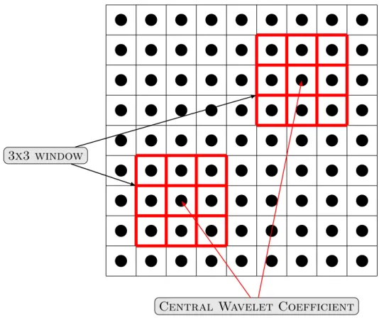
Statistical estimation provides estimates for the model’s parameters when given a statistical model and ML estimation applied to a data set. The distribution parameter σZ is standard deviation. A local adaptive technique gives superior performance if it is used to estimate the parameter in terms of σZ of every coefficient. Local neighborhood is a square window centered at the wavelet coefficient to be estimated. Equation 3.8 show that ML estimator is applied for noisy coefficient: σZ = arg max σ Pb(b) = arg max σ Y i,j∈Z(i,j) Pb(b(i, j)) = arg max σ X i,j∈Z(i,j) logPb(b(i, j)) (3.8)
P indicate the pdf with zero mean and varianceσ2,Z(i,j) is theN×N neighborhood
window in the subband as shown in Figure 3.2 [10]. Statistical estimation model is depend on maximum a posteriori(MAP) estimator to evaluate the signal variance and a LMMSE is applied to compute the true wavelet coefficient for reconstructed denoised image.
New modified denoising algorithm perform in two steps. Initially it perform MAP estimation of the variance for each corrupted coefficient in prior model for
Central Wavelet Coefficient 3x3 window
Figure 3.2: Neighborhood window selection
variance and a local neighborhood. In next step the estimated value of signal variance and noise variance are provided in the equation of the LMMSE for getting the noise free coefficient as it is shown in figure 3.1.
3.2
Denoising Algorithm
Data: Image contaminated with additive Gaussian noise Result: Estimated noiseless image
1 Decompose the noisy image using Discrete wavelet transform(DWT) into
wavelet domain up to Jth decomposition level;
2 for Each subband (i.e.HH, HL, and LH) in decomposition level j do 3 Parameters Estimation signal variance and noise variance σ2
x and σn2 ,respectively;
4 Apply LMMSE estimator to obtain modified noiseless wavelet
coefficients.;
5 up to Jth decomposition levels repeat steps (3) and (4);
6 Restore the denoised data using inverse wavelet transform from the
modified coefficients;
Algorithm 1: Denoising Algorithm
3.3
Parameter Estimation
In this section parameters are estimated for noisy coefficients to extract the noiseless wavelet coefficients. Here signal and noise variance is estimated using MAP and ML estimation and then LMMSE method is applied,instead of thresholding.
This plans focused around the noise variance and size of the image for every subband. It provides better result in terms of PSNR when a more adaptive threshold is taken and local features of the signal are considered. The parameterσn is normally assessed with the scaled Median Absolute Deviation (MAD) estimator [31]. The MAD estimator is widely used in the denoising step. In DWT image is decomposed in different subband. Wavelet details coefficients ψHH1 of the finest
decomposition level are associated only to the noise. The MAD estimator uses the median of absolute value of ψHH1 coefficients to estimate noise variance. MAD
is especially useful for the sparse signals that have a very small amount of signal power in the detail subbands. MAD is defined in equation 3.9.
ˆ
σm = M AD(|ψ HH1|)
0.6745 (3.9)
where MAD is the median absolute deviation.
We introduce weighting factor g(k) to extract more noiseless coefficient of noisy wavelet coefficient for each decomposition levels. Then noise variance and signal variance is estimated as follows:
ˆ
σn2 = g(k)ˆσ2m (3.10) = 22kk+1σˆ2
m (3.11)
where value of k is taken as 2.
The signal variance of noiseless image is estimated as follows:
ˆ σx2 = σ2y −σˆm2 if σy2 >σˆm2 0 otherwise (3.12) σ2y = 1 M.N M X m=1 N X n=1 w2(m, n) (3.13)
wherewis wavelet coefficient in the square neighborhood at each scale,and M×N is the size of test image.
3.4
Experiment and Results
This section discussed the results of the proposed schemes.This technique is applied on various images taken from USC-SIPI image database [32]. This technique is applied on miscellaneous images like Lena, Cameraman, Barbara, and house Figure 3.3 are used for experimental purpose. This section compares the other existing denoising schemes with proposed scheme. Four standard gray scale images (Lena, Cameraman, Barbara, and house) of size 256× 256 are contaminated with zero mean Gaussian noise (σ = 10,20,30,50, and100) and
then denoised using various methods, including the one proposed by us. We have taken local window of size 3×3 using CDF(1,4) wavelet basis function up to 4 decomposition levels.
Two performance table 3.2 and 3.1 shows result of reconstructed image measured and compared here in terms of structural similarity index(SSIM) and peak signal-to -noise ratio (PSNR) respectively.
Four plots 3.14, 3.15, 3.16, 3.17 show the curve drawn between PSNR and Noise Level, and all graph compare the PSNR result of proposed method with existing denoising method . It observed that the Proposed scheme works well
(a) (b)
(c) (d)
Figure 3.3: Four 256×256 test images taken for experiment purpose(a) Lena.(b) House.(c) Barbara.(d) Cameraman.
for all four images in terms of PSNR when noise level is considered as (σ = 10,20,30,50, and100).
(a) (b)
(c) (d)
(e) (f)
Figure 3.4: (a) Noisy Lena with (σ= 20) (b) Denoised using neighshrink (28.56db) (c)Denoised using Bivariate (30.50db) (d) Denoised using GIDNWC (29.22db) (e)Denoised using IAWDMBNC (29.56db) (f)Denoised Image using MLMMSE (30.74db) .
(a) (b)
(c) (d)
(e) (f)
Figure 3.5: (a)Cameraman Image with noise level (σ = 20) (b) Denoised using neighshrink (26.44db) (c)Denoised using Bivariate (30.23db) (d) Denoised using GIDNWC (27.42db) (e)Denoised using IAWDMBNC (27.76db) (f)Denoised using MLMMSE (30.40db) .
(a) (b)
(c) (d)
(e) (f)
Figure 3.6: Denoised Lena images(a) Noisy Lena Image (σ = 10) (c) Noisy Lena Image (σ = 20) (e) Noisy Lena Image (σ = 30) (b),(d),(f) Denoised Images by Proposed Method.
(a) (b)
(c) (d)
Figure 3.7: Denoised Lena images (a) Noisy Lena Image (σ = 50) (c) Noisy Lena Image (σ = 100) (b),(d) Denoised Images by Proposed Method.
(a) (b)
(c) (d)
(e) (f)
Figure 3.8: Denoised Cameraman images (a) Noisy Cameraman Image (σ = 10) (c) Noisy Cameraman Image (σ = 20) (e) Noisy Cameraman Image (σ = 30) (b),(d),(f) Denoised Images by Proposed Method.
(a) (b)
(c) (d)
Figure 3.9: Denoised Cameraman images (a) Noisy Cameraman Image (σ = 50) (c) Noisy Cameraman Image (σ = 100) (b),(d) Denoised Images by Proposed Method.
(a) (b)
(c) (d)
(e) (f)
Figure 3.10: Denoised House images (a) Noisy House Image (σ = 10) (c) Noisy House Image (σ = 20) (e) Noisy House Image (σ = 30) (b),(d),(f) Denoised Images by Proposed Method.
(a) (b)
(c) (d)
Figure 3.11: Denoised House images (a) Noisy House Image (σ = 50) (c) Noisy House Image (σ = 100) (b),(d) Denoised Images by Proposed Method.
(a) (b)
(c) (d)
(e) (f)
Figure 3.12: Denoised Barbara images (a) Noisy Barbaran Image (σ = 10) (c) Noisy Barbara Image (σ = 20) (e) Noisy Barbaran Image (σ = 30) (b),(d),(f) Denoised Images by Proposed Method.
(a) (b)
(c) (d)
Figure 3.13: Denoised Barbara images (a) Noisy Barbara Image (σ = 50) (c) Noisy Barbara Image (σ = 100) (b),(d) Denoised Images by Proposed Method.
Table 3.1: PSNR(dB) Image Denoising Performance Table For Lena, Cameraman, Barbara, and house images
Denoising Algorithms
Images Noise Levels
Neighshrink Bivariate GIDNWC IAWDMBNC MLMMSE
Lena 10 33.21 34.18 33.65 33.83 34.36 20 28.56 30.50 29.22 29.56 30.74 30 26.06 28.33 26.74 27.44 28.83 50 23.10 25.55 24.01 24.33 26.64 100 22.10 21.20 22.30 22.40 23.81 Barbara 10 31.05 32.17 31.76 32.45 32.73 20 25.26 28.09 25.95 27.73 28.57 30 22.57 25.84 23.01 24.59 26.33 50 21.07 23.21 21.10 22.60 24.29 100 20.18 19.17 20.05 20.37 22.44 Cameraman 10 32.23 34.12 33.45 33.67 34.16 20 26.44 30.23 27.42 27.76 30.40 30 24.23 27.89 25.04 25.46 27.33 50 21.44 24.92 22.67 23.55 24.91 100 19.23 20.70 19.67 20.54 22.05 House 10 32.45 34.23 33.43 34.03 35.14 20 30.34 31.14 31.95 31.64 32.08 30 27.12 29.64 28.54 29.34 30.40 50 23.45 26.34 26.54 25.97 27.88 100 20.34 23.04 22.12 22.83 24.96
Table 3.2: SSIM Image Denoising Performance Table For Lena, Cameraman, Barbara, and house
Denoising Algorithms
Images Noise Levels
Neighshrink Bivariate GIDNWC IAWDMBNC MLMMSE
Lena 10 0.87 0.86 0.88 0.89 0.89 20 0.78 0.80 0.80 0.81 0.82 30 0.71 0.73 0.73 0.71 0.72 50 0.64 0.60 0.66 0.67 0.6 100 0.60 0.40 0.62 0.61 0.61 Barbara 10 0.88 0.90 0.89 0.90 0.91 20 0.70 0.83 0.73 0.74 0.80 30 0.56 0.72 0.73 0.63 0.69 50 0.49 0.58 0.52 0.55 0.63 100 0.47 0.38 0.48 0.47 0.50 Cameraman 10 0.90 0.91 0.90 0.91 0.92 20 0.78 0.82 0.84 0.82 0.84 30 0.72 0.73 0.74 0.74 0.72 50 0.66 0.67 0.60 0.68 0.66 100 0.590 0.59 0.58 0.57 0.61 House 10 0.83 0.84 0.85 0.82 0.85 20 0.76 0.77 0.78 0.77 0.80 30 0.71 0.72 0.71 0.71 0.76 50 0.65 0.67 0.65 0.70 0.70 100 0.60 0.60 0.62 0.61 0.63
10 20 30 40 50 60 70 80 90 100 14 16 18 20 22 24 26 28 30 32 34 36 Noise Level P S N R in d b Lena Image MLMMSE Neighshrink Bivariate GIDNWC IAWDMBNC
Figure 3.14: Denoising performance comparison of Lena image
10 20 30 40 50 60 70 80 90 100 14 16 18 20 22 24 26 28 30 32 34 36 Noise Level P S N R in d b Barbara Image MLMMSE Neighshrink Bivariate GIDNWC IAWDMBNC
10 20 30 40 50 60 70 80 90 100 14 16 18 20 22 24 26 28 30 32 34 36 Noise Level P S N R in d b Cameraman Image MLMMSE Neighshrink Bivariate GIDNWC IAWDMBNC
Figure 3.16: Denoising performance comparison of Cameraman image
10 20 30 40 50 60 70 80 90 100 14 16 18 20 22 24 26 28 30 32 34 36 Noise Level P S N R in d b House Image MLMMSE Neighshrink Bivariate GIDNWC IAWDMBNC
Conclusions and Future Scope
This chapter concludes the overall examination about this thesis and recommends some of the future works in the research area of image denoising Section 5.1 gives the conclusion of proposed image denoising technique. Section 4.2 shows the future scope for extending the proposed technique.
4.1
Conclusion
In this thesis, image denoising using discrete wavelet transform has been discussed.In the first part of thesis ,we have introduced some important wavelet transform for image denoising.Then the existing denoising algorithms using various different approaches have been described as a literature review.
In the latter part of the thesis ,we have proposed new parameter estimation for LMMSE estimator for image denoising. Various estimation expression and different experimental results can be obtained by statistical estimation model.This scheme give fairly satisfying results in both PSNR and SSIM comparison aspects and outperform some existing algorithm as listed in the experimental results.
4.2
Future Scope
This thesis has opened several well known algorithms for denoising natural images and their performance was comparatively assessed in the research directions which have scope of further investigation. This proposed can be extended to color image.The LMMSE estimator can be used by optimizing Statistical Modeling.This technique can be extended to video denoising and can be used for color videos.
[1] Rafael C. Gonzalez, Richard E. Woods (2007). Digital Image Processing. Pearson Prenctice Hall. ISBN 0-13-168728-X.
[2] Jansen, Maarten. Noise reduction by wavelet thresholding. Vol. 61. New York: Springer, 2001.
[3] Donoho, David L. ”De-noising by soft-thresholding.” Information Theory, IEEE Transactions on 41.3 (1995): 613-627.
[4] Mallat, Stphane. A wavelet tour of signal processing. Academic press, 1999.
[5] David L. Donoho. ”Unconditional bases are optimal bases for data compression and for statistical estimation.” Applied and Computational Harmonic Analysis, Vol. 1, No. 1, pp. 100-115, Dec. 1993.
[6] Donoho, David L., and Iain M. Johnstone. ”Adapting to unknown smoothness via wavelet shrinkage.” Journal of the american statistical association 90.432 (1995): 1200-1224. [7] Zhang, D., Paul Bao, and Xiaolin Wu. ”Multiscale LMMSE-based image denoising with
optimal wavelet selection.” Circuits and Systems for Video Technology, IEEE Transactions on 15.4 (2005): 469-481.
[8] Coifman, Ronald R., and David L. Donoho. Translation-invariant de-noising. Springer New York, 1995.
[9] Chang, S. Grace, Bin Yu, and Martin Vetterli. ”Adaptive wavelet thresholding for image denoising and compression.” Image Processing, IEEE Transactions on 9.9 (2000): 1532-1546.
[10] Om, Hari, and Mantosh Biswas. ”A generalized image denoising method using neighbouring wavelet coefficients.” Signal, Image and Video Processing (2013): 1-10.
[11] Sendur, Levent, and Ivan W. Selesnick. ”Bivariate shrinkage with local variance estimation.” Signal Processing Letters, IEEE 9.12 (2002): 438-441.
[12] Pizurica, Aleksandra, et al. ”A joint inter-and intrascale statistical model for Bayesian wavelet based image denoising.” Image Processing, IEEE Transactions on 11.5 (2002): 545-557.
[13] Hou, Zujun. ”Adaptive singular value decomposition in wavelet domain for image denoising.” Pattern Recognition 36.8 (2003): 1747-1763.
[14] Boubchir, Larbi, and Boualem Boashash. ”Wavelet denoising based on the MAP estimation using the BKF prior with application to images and EEG signals.” (2013): 1-1.
[15] Zhang, Guo-Duo, et al. ”Image denoising based on support vector machine.” Engineering and Technology (S-CET), 2012 Spring Congress on. IEEE, 2012.
[16] Chen, G. Y., Tien D. Bui, and Adam Krzyzak. ”Image denoising using neighbouring wavelet coefficients.” Integrated Computer-Aided Engineering 12.1 (2005): 99-107.
[17] Chen, G. Y., and T. D. Bui. ”Multiwavelets denoising using neighboring coefficients.” Signal Processing Letters, IEEE 10.7 (2003): 211-214.
[18] Ruikar, Sachin, and D. D. Doye. ”Image denoising using wavelet transform.”Mechanical and Electrical Technology (ICMET), 2010 2nd International Conference on (pp 509-515).IEEE, 2010.
[19] Jain AK. Fundamental of digital image processing.Prentice Hall;Upper Saddle River,NJ;2001.
[20] Liua, Jia, Caicheng Shi, and Meiguo Gao. ”Image denoising based on BEMD and PDE.” Computer Research and Development (ICCRD), 2011 3rd International Conference on. Vol. 3. IEEE, 2011.
[21] Om, Hari, and Mantosh Biswas. ”MMSE based map estimation for image denoising.” Optics Laser Technology 57 (2014): 252-264.
[22] Jiang, Jun, et al. ”An improved adaptive wavelet denoising method based on neighboring coefficients.” Intelligent Control and Automation (WCICA), 2010 8th World Congress on. IEEE, 2010.
[23] Donoho, David L. ”Unconditional bases are optimal bases for data compression and for statistical estimation.” Applied and computational harmonic analysis 1.1 (1993): 100-115. [24] Mallat, Stephane G. ”A theory for multiresolution signal decomposition: the wavelet representation.” Pattern Analysis and Machine Intelligence, IEEE Transactions on 11.7 (1989): 674-693.
[25] Abramovich, Felix, Theofanis Sapatinas, and Bernard W. Silverman. ”Wavelet thresholding via a Bayesian approach.” Journal of the Royal Statistical Society: Series B (Statistical Methodology) 60.4 (1998): 725-749.
[26] Kivanc Mihcak, M., et al. ”Low-complexity image denoising based on statistical modeling of wavelet coefficients.” Signal Processing Letters, IEEE 6.12 (1999): 300-303.
[27] E. W. Karmen and J. K. Su, Introduction to Optimal Estimation.London, U.K.: Springer-Verlag, 1999.
[28] Gauvain, Jean-Luc, and Chin-Hui Lee. ”Maximum a posteriori estimation for multivariate Gaussian mixture observations of Markov chains.” Speech and audio processing, ieee transactions on 2.2 (1994): 291-298.
[29] Synyavskyy, Andriy, Sviatoslav Voloshynovskiy, and Ivan Prudyus. ”Wavelet-based map image denoising using provably better class of stochastic IID image models.” Facta Universitatis 14 (2001).
[30] Wang, Zhou, et al. ”Image quality assessment: from error visibility to structural similarity.” Image Processing, IEEE Transactions on 13.4 (2004): 600-612.
[31] Donoho, David L. and Jain M. Johnstone. ”Ideal spatial adaptation by wavelet shrinkage.” Biometrika 81.3 (1994): 425-455.