Development and optimisation of chemometric techniques for the evaluation of meat freshness

(1)

CRANFIELD UNIVERSITY

Eleni Anthippi Chatzimichali

Development and Optimisation of Chemometric Techniques

for the Evaluation of Meat Freshness

Cranfield Health

PhD Thesis

Supervisor: Professor Conrad Bessant

2013

(2)

CRANFIELD UNIVERSITY

CRANFIELD HEALTH

PHD THESIS

2013

ELENI ANTHIPPI CHATZIMICHALI

Development and Optimisation of Chemometric Techniques

for the Evaluation of Meat Freshness

Supervisor:

Professor Conrad Bessant

(3)

ABSTRACT

Muscle foods such as meat, fish and poultry are an integral part of human diet. Over time, such food succumbs to spoilage, resulting from various intrinsic and extrinsic factors, the most significant of which is microbial activity. Spoilage changes the organoleptic properties of meat, rendering it unacceptable to the consumer, and may ultimate result in the food becoming toxic. Spoilage is therefore of major commercial and public health interest.

This thesis describes the development and application of a novel suite of software tools designed to support novel instrumental approaches for the accurate, rapid and inexpensive evaluation of meat freshness. A pipeline was built for the analysis of highly heterogeneous data obtained by a diverse range of high-throughput techniques across four three-class case studies. As a first step, PCA was applied for dimensionality reduction, feature extraction and exploratory analysis. PLS-DA and SVMs were employed as classifiers, and classification ensembles implemented as a means of improving classification accuracy. Rigorous validation and evaluation methods based on bootstrapping and permutation testing were applied to ensure that the performance metrics are representative of real-world application, and to ascertain the statistical significance of the results. This was made possible by the development of an advanced optimisation approach, which reduced the computational demands of SVM tuning by up to ~ 90× times. The functionality of the pipeline was further enhanced by exploiting GPA and CPCA as data fusion techniques, to evaluate whether better classification accuracy is achieved when integrated as opposed to standalone datasets are used.

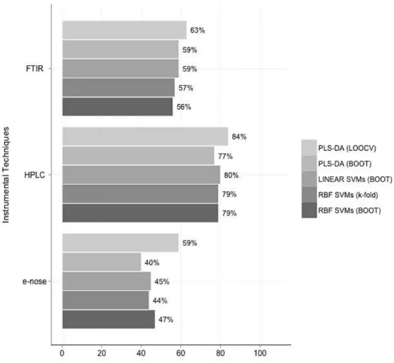
SVM ensembles proved to be the most powerful and accurate classification method since they produced consistently higher prediction rates ( ) than PLS-DA. Among the analytical techniques, HPLC was established as the most diagnostic method for the assessment of meat freshness, with a of 80%. Among the two data fusion techniques, CPCA outperformed GPA. However, CPCA only exceeded standalone HPLC in a minority of cases, presenting an overall of 82%.

(4)

ACKNOWLEDGMENTS

First and foremost, I would like to thank my supervisor Professor Conrad Bessant for his overwhelming contribution and support during this project. Your ever-present advice and guidance are worthy of my lasting gratitude. Thank you for the time and dedication you invest in me.

To my friends and colleagues in Cranfield University I declare my deep indebtedness for their wholehearted support. Thank you for providing me with the necessary impetus to better myself.

My deepest gratitude goes above all to my beloved parents. This project would have not been feasible without your ever-lasting support, trust and encouragement. A huge thank you for always being there for me.

(5)

TABLE OF CONTENTS

ABSTRACT ... iii

ACKNOWLEDGMENTS ... iv

TABLE OF CONTENTS ... v

TABLE OF FIGURES ... viii

TABLE OF TABLES ... xii

TABLE OF EQUATIONS ... xiii

ABBREVIATIONS ... xiv

1 Introduction and Literature Review ... 1

1.1 Introduction ... 1

1.1.1 Overview of Systems Biology ... 1

1.1.2 The ‘omics’ disciplines ... 3

1.1.3 Microbial Spoilage in Meat ... 6

1.2 Multivariate Analyses and Chemometrics ... 7

1.3 Data pre-treatment ... 8

1.3.1 Mean-centering ... 9

1.3.2 Auto-scaling ... 9

1.4 Multivariate Analysis: Unsupervised Methods ... 10

1.4.1 Principal Component Analysis ... 10

1.4.2 Cluster Analysis ... 12

1.5 Multivariate Analysis: Supervised Learning ... 14

1.5.1 Partial Least Squares – Discriminant Analysis... 14

1.5.2 Support Vector Machines ... 15

1.5.3 Ensemble Models ... 22

1.6 Validation ... 23

1.6.1 The holdout method ... 24

1.6.2 k-fold Cross-Validation ... 25

1.6.3 Leave-One-Out Cross-Validation ... 26

1.6.4 Bootstrapping ... 27

1.6.5 Model Selection, complexity and the bias-variance trade-off ... 27

1.7 Permutation Tests ... 29

1.8 Aims and objectives ... 30

2 Development of the multivariate analysis pipeline for the detection of meat spoilage ... 32

2.2 Materials and Methods ... 32

2.2.1 Case study 1: “Shelf life beef fillets stored in air at 0, 5, 10, 15 and 20°C” 32 2.2.2 Data pre-Processing and Dimensionality Reduction ... 37

2.2.3 Standalone Classifiers: PLS-DA models with LOOCV ... 38

2.2.4 Ensemble of Classifiers ... 39

2.2.5 The Architecture ... 42

2.2.6 Implementation in R ... 43

2.3 Results and Discussion ... 44

2.3.1 Principal Component Analysis ... 44

(6)

2.4 Conclusion ... 57

3 Optimisation of the RBF SVM tuning process via bootstrapping ... 59

3.2.1 Parallel Computing ... 59

3.2.2 Approximation Algorithms ... 61

3.2.3 Nelder-Mead Simplex Algorithm ... 63

3.2.4 Box Constrained Simplex Algorithm ... 64

3.3.1 Linear Models ... 66

3.3.2 Nonlinear Models ... 68

4 Integration of Heterogeneous Data ... 80

4.2.1 Data Integration ... 80

4.2.2 Procrustes Analysis ... 82

4.2.3 Generalised Procrustes Analysis ... 83

4.2.4 Multi-block Principal Component Analysis ... 85

4.2.5 Data Integration and Analysis Pipeline ... 88

4.3.1 Exploratory Data Analysis ... 91

4.3.2 Classification Results ... 93

4.3.3 Permutation Tests ... 102

5 Application of the multivariate analysis pipeline on new case studies ... 112

5.2.1 Case study 2: “Shelf life of minced beef stored in air, MAP, and in active packaging at 0, 5, 10 and 15oC” ... 113

5.2.2 Case study 3: “Survey of minced beef” ... 115

5.2.3 Case study 4: “Pork stored in air and MAP” ... 118

5.2.4 The architecture ... 120

5.3.1 Case study 2 ... 121

5.3.2 Case study 3 ... 134

5.3.3 Case study 4 ... 146

5.4 Comparison of the individual case studies ... 166

6 Development of improved visualisation methods for chemometrics applications 170 6.1 Introduction ... 170

6.2.1 The importance of Data Visualisation ... 170

6.2.2 Generating static graphs ... 172

(7)

6.2.4 The iWebPlots package ... 181

6.2.5 Constructing a web interface for demonstrative purposes... 183

7 Conclusion and Recommendations ... 195

7.1 Summary ... 195

7.2 Recommendations for Future Work ... 199

7.2.1 Improved classification of semi-fresh samples ... 199

7.2.2 Improvement of the SVM optimisation algorithm ... 200

7.2.3 Feature extraction ... 201

(8)

TABLE OF FIGURES

Figure 1-1 Evolution from molecular biology to systems biology ... 2

Figure 1-2 Electromagnetic spectrum ... 4

Figure 1-3 Representation of possible correlations and redundancies in high-dimensional data ... 10

Figure 1-4 Extracting the Principal Components ... 11

Figure 1-5 Nonlinear SVM classifier ... 18

Figure 1-6 The effect of the hyperparameter on the SVM boundaries ... 21

Figure 1-7 k-fold Cross-Validation... 25

Figure 1-8 Leave-One-Out Cross Validation (LOOCV) ... 26

Figure 1-9 Model complexity and overfitting; the bias-variance trade-off ... 28

Figure 1-10 Permutation tests and the P-value ... 29

Figure 2-1 Mean FTIR spectra for case study 1 in the fingerprint region (1500-1000 cm-1) ... 35

Figure 2-2 Sampling with Libra e-nose ... 36

Figure 2-3 Data intersection ... 38

Figure 2-4 The process of constructing an ensemble of RBF SVMs optimised via bootstrapping ... 42

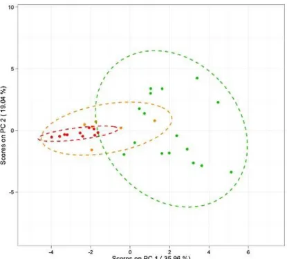
Figure 2-5 PCA score plots with 95% confidence ellipses for case study 1 ... 46

Figure 2-6 Overall accuracies (%CC) for the standalone datasets of case study 1 ... 49

Figure 2-7 Class prediction rates of the standalone (prior to PCA) datasets for case study 1 ... 52

Figure 2-8 Comparison of the optimisation of the hyperparameters of RBF SVMs via bootstrapping, 10-fold cross-validation and LOOCV respectively ... 55

Figure 2-9 Three-dimensional error surface plots for the optimisation of the RBF parameters ... 56

Figure 3-1 Master/Slave architecture ... 60

Figure 3-2 Embarrassingly parallel problems in the analysis pipeline ... 61

Figure 3-3 The steps of the Nelder-Mead algorithm ... 64

Figure 3-4 The relationship between the number of slave processors (master/slave model) and the execution times of an ensemble of PLS-DA with bootstrapping 67 Figure 3-5 Step-by-step representation of the Box complex algorithm towards identifying the optimal hyperparameters and the minimum bootstrapping error (HPLC data) ... 70

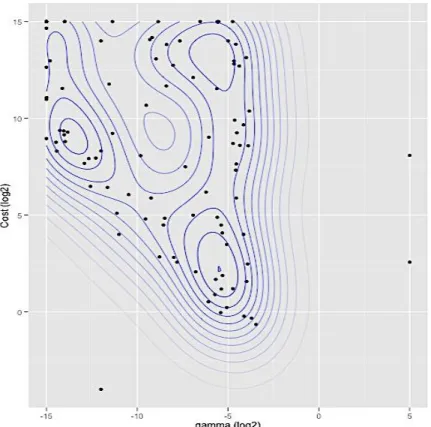
Figure 3-6 Contour plots of the density estimation of the optimal hyperparameters as defined by the Box complex algorithm ... 71

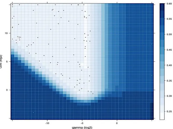
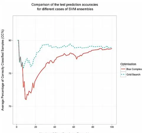
Figure 3-7 Density, filled-contour, grid and contour plots for the HPLC optimisation 72 Figure 3-8 Comparison of the prediction accuracies between the grid-Search and the Box complex algorithm (HPLC data) ... 73

Figure 3-9 Histograms of the number of iterations and function evaluations respectively for an ensemble of nonlinear (RBF) SVMs optimised using the Box complex algorithm. ... 74

Figure 3-10 Comparison of the execution times for the tuning of a single RBF SVM ensemble, when optimised with different techniques, via bootstrapping ... 76

Figure 3-11 Comparison of the execution times of 100 permutation tests for the (RBF) SVMs when optimised with different techniques, via bootstrapping ... 77

(9)

Figure 3-12 Speedup produced by the different optimisation techniques ... 78

Figure 4-1 Procrustes Analysis superimposition ... 82

Figure 4-2 Generalised Procrustes Analysis ... 84

Figure 4-3 Steps of CPCA for the datasets of case study 1 ... 86

Figure 4-4 Data integration workflow ... 90

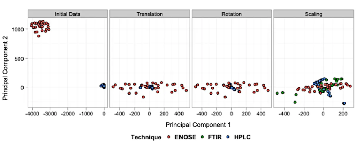
Figure 4-5 The steps of GPA (shown in order from left to right) when applied on the datasets of case study 1 ... 91

Figure 4-6 The consensus of the first two Principal Components based on the fusion of all three experimental techniques of case study 1 using GPA and CPCA respectively ... 92

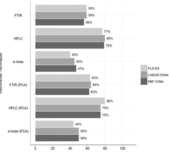
Figure 4-7 Overall accuracies (%CC) for the standalone datasets of case study 1 ... 95

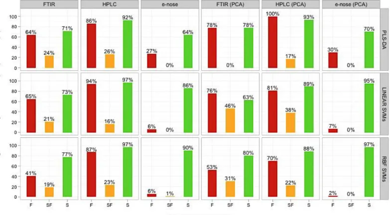
Figure 4-8 Classification Results for the integrated datasets of case study 1... 96

Figure 4-9 Class prediction rates of the standalone (prior and after PCA) datasets for case study 1 ... 100

Figure 4-10 Class prediction rates of the integrated datasets for case study 1 ... 101

Figure 4-11 Distribution plots of the permutation tests on the datasets of case study 1 using nonlinear (RBF) SVMs ... 105

Figure 4-12 Distribution plots of the permutation tests on the data of case study 1 using PLS-DA ... 106

Figure 4-13 Superimposed density plots of the permutation tests on the datasets of case study 1 using PLS-DA and nonlinear (RBF) SVMs ... 107

Figure 4-14 Boxplots representing the outcome of permutation testing when PLS-DA and RBF SVMs are applied on the datasets of case study 1 ... 110

Figure 5-3 Mean Raman spectra for case study 3 in the range 200-3400 cm-1 ... 117

Figure 5-5 PCA scores plots with 95% confidence ellipses for case study 2 ... 123

Figure 5-6 The consensus of the first two Principal Components based on the fusion of the two experimental techniques from case study 2 using GPA and CPCA respectively ... 124

Figure 5-7 Overall accuracies (%CC) for the standalone and integrated datasets of case study 2 ... 126

Figure 5-8 Class prediction rates of the standalone (prior and after PCA) and integrated datasets for case study 2 ... 128

Figure 5-9 Distribution plots of the permutation tests on the datasets of case study 2 using RBF SVMs and PLS-DA respectively ... 130

Figure 5-10 Superimposed density plots of the permutation tests on the datasets of case study 2 using PLS-DA and nonlinear (RBF) SVMs ... 131

Figure 5-11 Boxplots representing the outcome of permutation testing when RBF SVMs and PLS-DA are applied on the datasets of case study 2 ... 133

Figure 5-12 Execution times of the permutation tests on the datasets of case study 2 ... 134

(10)

Figure 5-14 The consensus of the first two Principal Components based on the fusion of the two experimental techniques from case study 3 using GPA and CPCA respectively ... 137 Figure 5-15 Overall accuracies (%CC) for the standalone and integrated datasets of

case study 3 ... 139 Figure 5-16 Class prediction rates of the standalone (prior and after PCA) and

integrated datasets for case study 3 ... 140 Figure 5-17 Distribution plots of the permutation tests on the datasets of case study 3

using RBF SVMs and PLS-DA respectively ... 142 Figure 5-18 Superimposed density plots of the permutation tests on the datasets of

case study 3 using PLS-DA and nonlinear (RBF) SVMs ... 143 Figure 5-19 Boxplots representing the outcome of permutation testing when RBF

SVMs and PLS-DA are applied on the datasets of case study 3 ... 145 Figure 5-20 Execution times of the permutation tests on the datasets of case study 3

... 146 Figure 5-21 PCA scores plots with 95% confidence ellipses for case study 4 ... 149 Figure 5-22 The consensus of the first two Principal Components based on the fusion

of the two experimental techniques of case study 4 using GPA and CPCA

respectively ... 150 Figure 5-23 Overall accuracies (%CC) for the standalone datasets of case study 4 .. 153 Figure 5-24 Classification Results for the integrated datasets of case study 4... 154 Figure 5-25 Class prediction rates of the standalone (prior and after PCA) datasets for

case study 4 ... 156 Figure 5-26 Class prediction rates of the integrated datasets for case study 4 ... 157 Figure 5-27 Distribution plots of the permutation tests on the datasets of case study 4

using RBF SVMs ... 159 Figure 5-28 Distribution plots of the permutation tests on the data of case study 4

using PLS-DA ... 160 Figure 5-29 Superimposed density plots of the permutation tests on the datasets of

case study 4 using PLS-DA and nonlinear (RBF) SVMs ... 161 Figure 5-30 Boxplots representing the outcome of permutation testing when RBF

SVMs and PLS-DA are applied on the datasets of case study 4 ... 164 Figure 5-31 Execution times of the permutation tests on the datasets of case study 4

... 165 Figure 5-32 Investigating the common trends across all four individual case studies168 Figure 6-1 The “designer-reader-data trinity” of data visualisation ... 171 Figure 6-2 Construction process of a ggplot2 graph – the layered grammar approach

... 174 Figure 6-3 The workflow from Sweave to an automatically generated PDF file... 176 Figure 6-4 The progress of web technologies and programming languages over time

... 178 Figure 6-5 Comparison between the classic and the AJAX web application model .. 180 Figure 6-6 Scatterplots produced by the graphics and ggplot2 package respectively 186 Figure 6-7 Scatterplots with density estimation using the KernSmooth and ggplot2

packages... 187 Figure 6-8 Comparison of static data representation and powerful feature-rich

(11)

Figure 6-9 Sweave example for the dynamic construction of a PDF report directly from R ... 191 Figure 6-10 Interactive dendrogram generated by the iWebPlots package representing

the outcome of HCA when applied on the HPLC data of case study 1 ... 192 Figure 6-11 Partial view of the implemented web interface for the FTIR dataset of case

(12)

TABLE OF TABLES

Table 1 The sizes and data composition of standalone datasets from case study 1 prior to analysis ... 37 Table 2 PCA proportion and cumulative variance captured for the datasets of case

study 1 ... 44 Table 3 Descriptive statistics of the permutation distributions obtained by RBF SVMs (case study 1) ... 108 Table 4 Descriptive statistics of the permutation distributions obtained by PLS-DA

(case study 1) ... 109 Table 5 The sizes and data composition of standalone datasets from case study 2 prior

to analysis ... 115 Table 6 The sizes and data composition of standalone datasets from case study 3 prior

to analysis ... 118 Table 7 The sizes and data composition of standalone datasets from case study 4 prior

to analysis ... 120 Table 8 PCA proportion and cumulative variance captured for the datasets of case

study 2 ... 121 Table 9 Descriptive statistics of the permutation distributions obtained by RBF SVMs

(case study 2) ... 132 Table 10 Descriptive statistics of the permutation distributions obtained by PLS-DA

(case study 2) ... 132 Table 11 PCA proportion and cumulative variance captured for the datasets of case

study 3 ... 135 Table 12 Descriptive statistics of the permutation distributions obtained by RBF

SVMs (case study 3) ... 144 Table 13 Descriptive statistics of the permutation distributions obtained by PLS-DA

(case study 3) ... 144 Table 14 PCA proportion and cumulative variance captured for the datasets of case

study 4 ... 147 Table 15 Descriptive statistics of the permutation distributions obtained by RBF

SVMs (case study 4) ... 162 Table 16 Descriptive statistics of the permutation distributions obtained by PLS-DA

(13)

TABLE OF EQUATIONS

Equation 1 Mean-centering formula ... 9

Equation 2 Auto-scaling formula ... 9

Equation 3 PCA scores and loadings ... 11

Equation 4 Euclidean distance algorithm ... 12

Equation 5 Single linkage algorithm ... 13

Equation 6 k-means clustering algorithm ... 13

Equation 7 Partial Least Squares - Discriminant Analysis ... 15

Equation 8 Linear SVM classifier as a decision function ... 15

Equation 9 SVM linear separating hyperplane ... 16

Equation 10 SVM supporting hyperplanes ... 16

Equation 11 SVM optimisation problem – primal form (hard-margin SVMs) ... 16

Equation 12 SVM optimisation problem – primal form (soft-margin SVMs) ... 17

Equation 13 SVM optimisation problem – dual form ... 17

Equation 14 SVM optimisation problem – primal form (kernel trick) ... 19

Equation 15 SVM optimisation problem – dual form (kernel trick) ... 19

Equation 16 Nonlinear SVM kernels ... 19

Equation 17 Percentage of correctly classified samples (%CC) ... 23

Equation 18 Root Mean Square Error ... 23

Equation 19 Box complex algorithm ... 64

Equation 20 Procrustes Analysis rotation criterion ... 83

Equation 21 Procrustes Analysis asymmetric dissimilarities ... 83

Equation 22 Procrustes rotation criterion in GPA ... 83

Equation 23 Generalised Procrustes Analysis criterion using a consensus ... 84

(14)

ABBREVIATIONS

%CC AJAX ATR CPCA CSS CSV DNA DOM E-NOSE FTIR GPA HCA HPLC HTML HTTP LOOCV LV MAP NIPALS OPA PC PCA PCR Perl PLS PLS-DA PNG RBF RIA

Percentages of Correctly Classified Samples Asynchronous JavaScript and XML

Attenuated Total Reflectance

Consensus Principal Component Analysis Cascading Style Sheet

Comma Separated File Deoxyribonucleic Acid Document Object Model Electronic Nose

Fourier Transform infrared (spectroscopy) Generalized Procrustes Analysis

Hierarchical Cluster Analysis

High Performance Liquid Chromatography HyperText Markup Language

HyperText Transfer Protocol Leave-One-Out Cross-Validation Latent Variable

Modified Atmosphere Packaging

Non-linear Iterative Partial Least Squares Ordinary Procrustes Analysis

Principal Component

Principal Component Analysis Polymerase Chain Reaction

Practical Extraction and Reporting Language Partial Least Squares

Partial Least Squares Discriminant Analysis Portable Network Graphics

Radial Basis Function Rich Internet Application

(15)

RMSE RMSECV SSE SVD SVMs SYMBIOSIS-EU XHTML XML WWW

Root Mean Square Error

Root Mean Square Error of Cross-Validation Sum of Squared Errors

Singular Value Decomposition Support Vector Machines

Scientific sYnerganisM of nano-Bio-Info-cOngi Science for an Integrated system to monitor meat quality and Safety during production, storage, and distribution in the European Union

Extensible HyperText Markup Language Extensible Markup Language

(16)

1 Introduction and Literature Review

1.1 Introduction

1.1.1 Overview of Systems Biology

Breakthrough biological discoveries over the past decades, such as the revolutionary discovery of the double helix structure of DNA in 1953 by Watson and Crick, catalysed the blossoming of molecular biology (Watson and Crick, 1953). Acquiring information about the structure and properties of DNA and proteins led to outstanding progress in the years that followed as presented in Figure 1-1. Molecular biology has chiefly focused on identifying and investigating individual biological molecules by studying their properties and functions either as isolated entities or as small sets of components in very simple model systems. However, the reductionist approach adapted by molecular biology was not sufficient to interpret the intrinsic complexity of biological systems.

The Human Genome Project has profoundly altered the practice and view of contemporary biology (Hood, 2003; Venter et al., 2001). In the post-genome era, the massive amount of biological data acquired by the advance of high-throughput technologies led to the rapid shift of interest towards systems biology. The marked increase in the amount of genomic, proteomic and metabolomic data due to the constant improvements in high-throughput tools, has granted the scientific community the opportunity to study complex biological systems as an integrated whole. Thus, systems biology emerged as a necessity helping us understand these complex system dynamics, as these are the key to understanding life. Systems analysis has historically been applied in a plethora of scientific fields such as economics, physics, psychology and most recently biology, covering a multitude of different areas such as developmental biology, ecology and immunology (Westerhoff et al., 2004).

(17)

Figure 1-1 Evolution from molecular biology to systems biology

The line of inquiry represents the way mainstream molecular biology, under the pressure for system-level study, started investigating groups of molecules rather than single macromolecules, while simultaneously investigated their interactions. The figure has been adapted from Westhoff et al. (2004).

A system-level approach aims to generate novel technologies and effective tools based on the collection, integration, analysis, graphical visualisation, and ultimately modelling of biological information (Ideker et al., 2001; Hood, 2003). Mathematical modelling is the backbone of contemporary systems biology. To this day the term “mathematical” is usually hidden behind a “computational approach” (Mesarovic et al., 2005). A model is an effort to represent all the integrated highly heterogeneous information that derives from multiple experimental sources in an abstract manner. Current advances in systems biology and computing science are prompting scientists to use sophisticated mathematical models and powerful in silico simulations. Despite the continuous acquisition of new information as well as the overwhelming progress of computational and experimental methods, the high complexity of biological systems will always constitute an obstacle for the construction of a general, integrated and functionally meaningful model based on complete understanding (Butcher et al., 2004; Filkenstein et al., 2004).

(18)

1.1.2 The ‘omics’ disciplines

Ever since the first automated DNA sequencing machine (See Figure 1-1), there has been a tremendous increase in the development of high-throughput platforms leading to the accumulation of vast amounts of highly heterogeneous biological data. These large-scale sets of data and biological information have inspired several novel fundamental concepts – namely, the ‘omics’ disciplines. These disciplines propel systems-level understanding, having as a chief aim the simultaneous quantification and identification of the building blocks of a biological system such as genes, proteins or metabolites, as well as the investigation of the interactions among them such as protein-protein.

Three of the most important ‘omics’ sources are genomics, proteomics and metabolomics. The term genomics was established to denote the analysis of the entire genome – the complete genetic sequence – of an organism. In all cellular organisms, the genome is composed of deoxyribonucleic acid (DNA). Proteomics can be defined as the scientific field that focuses on the study of the proteome. The proteome is the entire collection of proteins that are expressed by a particular genome. However, even though the genome of a cellular organism is static – it alters only when mutations occur – the proteome changes constantly as a result of internal and external factors. Metabolomics is likewise defined as the comprehensive profiling of the metabolome. The metabolome consists of all the biochemicals and metabolites produced by a cellular organism. Metabolites are substances either required for or produced by biochemical reactions of metabolism that occur within the cells of an organism. Metabolomics allows scientists to study and compare the relationships between an organism’s genotype and phenotype, as well as the relationships between the genotype and the environment (Hassani et al., 2010).

This project will be focusing on the field of metabolomics, and in particular the study of metabolites responsible for meat spoilage. The analytical techniques that will be used in this project are briefly presented as follows.

(19)

1.1.2.1 Fourier Transform Infrared (FTIR) Spectroscopy

Fourier Transform Infrared (FTIR) spectroscopy is a very rapid (running over a few seconds) non-destructive analytical technique used for high-throughput biochemical fingerprinting (Ellis and Goodacre, 2001). In FTIR, a particular bond absorbs light or electromagnetic radiation by an infrared beam at a specific wavelength (Ellis et al., 2004). As a result of FTIR analysis, an infrared absorbance spectrum can be extracted, which may be used as a biochemical or metabolic “fingerprint” of the samples. However, FTIR spectra tend to be quite complex featuring hundreds or thousands of variables, thus necessitating the use of statistical methods for their analysis. FTIR in combination with multivariate statistical techniques has proven to be a very fast and accurate method for food-based analyses and bacterial detection (Nicolaou et al., 2011).

Figure 1-2 Electromagnetic spectrum

(20)

1.1.2.2 High Throughput Liquid Chromatography (HPLC)

High-performance liquid chromatography (HPLC) is a chromatographic technique used to separate a mixture of chemical compounds. It is mainly used in biochemistry and analytical chemistry to identify, quantify as well as purify the individual components in a mixture. The HPLC instrument consists of a solvent reservoir, transfer line with frit, high-pressure pump, sample injection device, column, detector, and data acquisition, usually together with data evaluation (Meyer, 2013)

1.1.2.3 Electronic Nose (e-nose)

An electronic nose (e-nose) is an instrument applied for the rapid non-destructive detection and analysis of microbial volatile compounds. The electronic noses attempt to mimic the human organoleptic olfactory interpretation (Persuad and Dodd, 1982). The instrument consists of an array of chemical gas sensors, which are capable of detecting and recognising simplex or complex odours.

Electronic noses have shown great promise in the field of food analysis as a means of evaluating freshness and investigating shelf life. E-noses have become increasingly popular due to the fact that they resemble human sensory evaluation, but also since they are rapid, low-cost non-destructive techniques. Even so, the repeatability with electronic noses has been questioned since they present instabilities due to severe instrumental drift (Ellis and Goodacre, 2001).

1.1.2.4 Raman Spectroscopy

Raman spectroscopy is also a non-destructive method that can be considered to be complementary to FTIR spectroscopy. Both Raman and FTIR are powerful metabolic fingerprinting methods as they reflect accurately the phenotype of a sample, including changes to its metabolism (Nicolaou et al., 2011). The major advantage of Raman spectroscopy over FTIR is the fact that the contribution from water is very small and thus can be used directly on food without recourse to ATR (Argyri et al., 2013).

(21)

1.1.3 Microbial Spoilage in Meat

Systems biology has gained in importance in food science and the food industry due to an increasing focus on food for better health and the demand for products of consistently high quality (Ellis et al.,2002; Hassani et al., 2010). Out of all foods that are a vital part of human diet, meat has been described as the most perishable of all. Muscle foods such as meat or poultry become unacceptable to the consumer when organoleptic changes occur due to spoilage (Ellis et al., 2002). Spoilage can be defined as “any change in a food product that renders it unacceptable to the consumer from a sensory point of view” (Gram et al., 2002; Ercolini et al., 2006)

Meat spoilage may be the result of a plethora of intrinsic and extrinsic factors, the most significant of which is microbial activity (Gram et al., 2002). Even though changes of food substances during storage may be the result of endogenous enzymatic processes within muscle tissue post-mortem, it is generally accepted that detectable organoleptic spoilage is a result of decomposition and the formation of metabolites caused by the growth of microorganisms (Ellis and Goodacre, 2001; Ellis et al., 2002). These organoleptic characteristics usually include the development of off-odours and off-flavours, the formation of slime in addition to any changes in the appearance such as discoloration; thus, consumers consider the meat as being undesirable. Due to its moist highly nutritious surface, meat stored at between -1 and 25°C favours the growth of a wide range of spoilage bacteria. Under aerobic conditions, spoilage organisms that belong primarily to the genus Pseudomonas attach more rapidly to meat surfaces than other spoilage bacteria (Ellis et al., 2002). The organoleptic changes may vary depending on the microbial association contaminating the meat and the conditions under which it is stored. The development of organoleptic spoilage is related to microbial consumption of meat nutrients such as sugars and free amino acids, and the release of undesired volatile metabolites (Ercolini et al., 2006).

(22)

Fears over microbiological food safety issues have led to the requirement for a rapid and accurate detection system for microbiologically spoiled or contaminated meat. To date, various methods have been proposed to measure and detect bacterial spoilage in meat such as enumeration methods based on microscopy, ATP bioluminescence and the measurement of electrical phenomena as well as detection methods based on immunological procedures (Ellis et al., 2002). However, these techniques are time-consuming, labour-intensive and generate retrospective information; thus, they cannot be used for on- or at-line monitoring (Ellis et al., 2002; Argyri et al., 2011). Polymerase chain reaction (PCR) techniques may also be investigated; however, the main limitation of these techniques is the high equipment cost, the demand for highly trained staff as well as the risk of cross-contamination (Nicolaou et al., 2011).

The research for reliable meat-quality sensors has led to the development of a plethora of rapid, non-invasive, and relatively inexpensive methods based on analytical instrumentation techniques such as Fourier transform infrared (FTIR) spectroscopy and electronic nose technology (Argyri et al., 2010; Panagou et al., 2010). The present study aims to develop an automated, reproducible and quantitative approach that defines the spoilage state of a product objectively. The application of analytical techniques such as the ones presented in Section 1.1.2 in conjunction with multivariate statistical techniques and machine learning algorithms may prove to be an effective, extremely fast and accurate method, which could have practical applications to ensure the quality and safety of meat and meat products.

1.2 Multivariate Analyses and Chemometrics

The vast amount of biological information generated by the advanced analytical instruments such as the omics fields, demand appropriate multivariate statistical tools for data analysis. Multivariate analysis can be defined as “the simultaneous statistical analysis of a collection of random variables” (Izenman, 2008). According to Vermuza and Filzmoser (2009), chemometrics may be defined as the “extraction of chemically relevant information out of analytical chemical data by mathematical and statistical tools”.

(23)

The multivariate techniques applied in the field of chemometrics are conventionally divided into two main categories, namely supervised and unsupervised. Unsupervised methods “attempt to disclose naturally occurring groups and structures within the dataset without previous knowledge of any class assignment” (Alvarez-Ordoñez and Prieto, 2012). They chiefly focus on the discovery of patterns, trends, clusters and/or outliers in the data, and they include techniques such as Principal Component Analysis (PCA) and cluster analysis. On the other hand, supervised learning algorithms “make use of a priori knowledge of classes to guide the characterisation or classification process” (Alvarez-Ordoñez and Prieto, 2012); these algorithms generate prediction models for regression, classification, pattern recognition, or machine learning tasks. Characteristic examples of supervised learning involve Partial Least Squares Discriminant Analysis (PLS-DA) and Support Vector Machines (SVMs), among many others.

1.3 Data pre-treatment

Nowadays, the extraction of relevant information from highly heterogeneous datasets constitutes a major challenge (van den Berg et al., 2006). It is well established that prior to the application of any type of data analysis, proper data pre-treatment is crucial for the outcome and the interpretability of the results. Data pre-treatment can make the difference between a useful model and no model at all. Therefore, biological data under investigation are often scaled, centered and/or transformed. The application of pre-treatment techniques may prove to be extremely fruitful, especially under circumstances where the variables span over wide and different ranges. In addition, pre-treatment techniques aim to minimise the influence of disturbing factors such as measurement noise.

The selection of chemometrics method to be applied, strongly influences the selection of the data pre-treatment methods. Different techniques focus on different aspects of the data. For instance, clustering algorithms focus on revealing similarity and dissimilarity patterns, whereas PCA attempts to explain the maximum variation based on a few meaningful components. Thus, a certain pre-treatment method may enhance the results of one technique and obscure the results of another.

(24)

1.3.1 Mean-centering

Mean-centering is conducted by subtracting the mean of each variable (column). “Centering converts all the concentrations to fluctuations around zero instead of around the mean” (van den Berg et al., 2006). This is step is usually performed so that all the components found by PCA have as their origin the centre (centroid) of the data (Craig et al., 2006). In general, mean-centering enhances the interpretability of a model; it can be useful when different variables have different means.

Equation 1 Mean-centering formula

1.3.2 Auto-scaling

In auto-scaling, also known as unit or unit variance scaling, each variable (column) is scaled to unit variance by using the standard deviation as the scaling factor. As the initial step, mean-centering is performed by subtracting the column mean from every data value. Subsequently, scaling is applied by dividing the centered columns by their standard deviation . Auto-scaling is crucial if different variables are measured over very different ranges or units such as temperature, pressure and concentration (Brereton, 2009). Once scaled, all the variables will have the same weight and will be equally important in the analysis (Wold et al., 2001; van den Berg et al., 2006). If the data are mean-centered, the weighting reflects the covariance of the variables, while in unit variance scaling the weighting reflects their correlation (Craig et al., 2006). The mathematical equation for auto-scaling is

( )

(25)

1.4 Multivariate Analysis: Unsupervised Methods

1.4.1 Principal Component Analysis

As thoroughly described in Section 1.1 scientists attempt via high-throughput platforms to collect as much information as possible from a single experiment. This may result in the generation of a large number of measurements (variables), a subset of which may not be very informative or even related to the study. Datasets with such great number of variables tend to present high dimensionality, correlations and redundancies. The plots of Figure 1-3 demonstrate three distinct cases, where the data illustrate low, medium and high redundancy respectively. The higher the redundancy, the more difficult it becomes to reveal patterns and trends in the original data.

Figure 1-3 Representation of possible correlations and redundancies in high-dimensional data For two random variables r1 and r2, the plot on the left displays no obvious relationship between the

variables. However, the variables of the plots in the centre and the right are highly correlated since one can be used to predict the other. The figure has been extracted from Shlens, 2005.

Principal Component Analysis (PCA) (Jackson, 1991; Wold et al., 1987) is the most commonly used technique for dimensionality reduction, data compression and feature extraction. The PCA algorithm reduces the initial number of possibly correlated variables into a new lower number of uncorrelated variables, known as the Principal Components (PCs). Geometrically, we can imagine the input data as a cloud of points in a high-dimensional space. As illustrated in Figure 1-4, this cloud of points is probably longer in a certain direction of the pattern space; in this direction the data appear to be most different and PCA draws the first axis (PC).

(26)

The first PC places all points the farthest apart from each other, extracting thus the highest variance. Similarly, a perpendicular to the first PC axis is drawn for the second PC, which accounts for the second highest variance. The process is repeated to get multiple orthogonal principal components. Each successive orthogonal axis displays a decreasing amount of the total variance.

Figure 1-4 Extracting the Principal Components

PCA projects the input data into a subspace of reasonable and meaningful dimension by setting new directions in the pattern space. Thus, the projected cloud of points is as dispersed as possible. The figure has been extracted from Kavraki (2007).

In matrix notation, suppose that variables have been observed on instances. The generated multivariate dataset forms an data matrix with rows (observations) and columns (variables). Thus, a cloud of points is created in an

-dimensional space, where a new axis is used per variable. The PCA algorithm reduces the size of possibly correlated variables into new uncorrelated variables (PCs), where . Each PC can be expressed mathematically as an orthogonal linear combination of the original variables . In PCA, the original matrix can be decomposed into the scores matrix , loadings matrix and a residuals matrix . Several algorithms can be used for data decomposition, the most widely applied of which are Singular Value Decomposition (SVD) and the Nonlinear Iterative Partial Least Squares (NIPALS) (Wold, 1975) algorithm. In general, the mathematical equation for PCA can be described by

(27)

1.4.2 Cluster Analysis

Cluster analysis consists of a set of unsupervised methods that are used in numerous data mining tasks. The clustering algorithms attempt to partition a dataset into several subsets – the clusters – so that data belonging to the same cluster are mutually similar, providing a sense of homogeneity.

1.4.2.1 Hierarchical Cluster Analysis (HCA)

Hierarchical clustering (HCA) is based on calculating the distances between elements found in a given matrix of size . The distances represent the degree of similarity/dissimilarity between these objects. The shorter the distance, the more similar the objects are with each other. HCA is based on two important categories of algorithms – distance and linkage algorithms.

Distance algorithms determine how the similarity or “distance measure” between two given objects is calculated. The most widely used distance algorithms include Euclidean and Mahalanobis distance, among others. For instance, for two objects and in , the Euclidean distance in -dimensional space satisfies the equation

√∑

Equation 4 Euclidean distance algorithm

Hierarchical clustering is graphically represented in tree structures, also known as dendrograms. Linkage algorithms determine how the clustering is performed. A bottom-up linkage algorithm includes the following steps:

1. Each object forms and belongs to its own cluster 2. The two closest clusters are linked together

3. The two linked clusters are aggregated into a single new cluster

(28)

Linkage algorithms consist of various different algorithms such as single linkage, complete linkage and Ward’s method. For two given clusters and , a single linkage algorithm calculates the shortest distance between the two clusters as described in Equation 5

‖ ‖ Equation 5 Single linkage algorithm

Where and are elements of the clusters and respectively.

1.4.2.2 -means Clustering

-means clustering is an unsupervised clustering technique that attempts to “minimise the sum of point-to-centroid distances, summed over all clusters” (Arthur and Vassilvitskii, 2007). The objective function for -means clustering is

∑ ∑‖ ‖

Equation 6 k-means clustering algorithm

Where, is the number of clusters, is the th pattern belonging to the th cluster, is the centre of cluster and is the number of data points. The algorithm’s steps can be described as follows:

1. Initially, the number of clusters is selected, for instance 2. Randomly the items are assigned to the clusters

3. A new centroid is calculated for each of the clusters (a distinct set of points belongs to a certain centroid)

4. The distance of each item towards the centroids is calculated 5. The items are subsequently assigned to the closest centroid

6. The algorithm keeps iterating until the assignments to the clusters are stable The algorithm’s simplicity and speed makes it an appealing technique for cluster analysis. However, a major disadvantage of this algorithm is that it is sensitive to the selection of the initial partitions.

(29)

1.5 Multivariate Analysis: Supervised Learning

This research will solely focus on the investigation of multivariate classification techniques. A classifier, also known as predictor, can be defined as “a function that maps an unlabelled instance to a label using internal data structures” (Kohavi, 1995). Supervised classification derives from the concept of learning by experience (Ciosek et al., 2005). A model is trained to distinguish groups of a predefined dataset where the class of each sample is already known. The training dataset is used to establish a mathematical model, which in turn should be capable of predicting the class membership of ideally unseen data (Izenman 2008). Supervised learning algorithms are characterised by a predefined set of parameters, which may have a profound effect on the resulting performance (Chapelle et al., 2002). Therefore, thorough selection of these parameters is a necessity.

1.5.1 Partial Least Squares – Discriminant Analysis

Partial Least Squares-Discriminant Analysis (PLS-DA) (Barker and Rayens, 2003) is a widely used classification technique in the field of chemometrics (Westerhuis et al., 2008). It is a linear model that consists of Partial Least Squares (PLS) (Wold, 1975) dimensionality reduction and Linear Discriminant Analysis (LDA) applied on the PLS components. Unlike PCA, which attempts to capture the maximum variance, PLS-DA aims to maximise the covariance – accomplish both correlation and maximum variance – between the input data and an output class (Wise et al., 2003; Weber et al., 2011).

In matrix notation, suppose that is a predictor matrix, which corresponds to independent variables, and is a class affiliation vector that holds the dependent variables. PLS-DA attempts to model the relationship between dependent and independent variables by projecting the data matrices and into a new subspace. The orthogonal axes in the PLS subspace are also known as Latent Variables (LVs). The output of PLS-DA is the product of two smaller matrices, the scores matrix (PLS-DA scores) and the predicted affiliation matrix. Thus, it satisfies the mathematical equations

(30)

Equation 7 Partial Least Squares - Discriminant Analysis

Where, represents the PLS score matrix, and are the PLS loadings, and and are the PLS residuals. Although the PLS scores (LVs) are orthogonal as in PCA, the loadings are not (Brereton, 2009). LVs are likely to offer a better separation between different observations (samples) when compared to PCs since they take the class labels into account (Rossini et al., 2012).

1.5.2 Support Vector Machines

Support Vector Machines (SVMs) (Boser et al., 1992; Cortes and Vapnik, 1995) are a powerful state-of-the-art machine learning technique applied in data mining cases such as classification, regression and novelty detection. Initially introduced by Cortes and Vapnik (1995) for binary classification (Hsu and Lin, 2002; Glasmachers, 2008), SVMs became increasingly popular in the scientific community over the past decade.

1.5.2.1 Linear SVM Classifiers: Separable Data

“The simplest type of classifier is a linear classifier” (Bottou et al., 1994; Brereton et al., 2009). In a hypothetical binary classification problem, the SVM model is given as input a training dataset , where is the set of input instances and their associated class labels. The chief goal of any SVM algorithm is to determine a classification function that best fits the training dataset. In the case of linearly separable points, the decision function has the form

〈 〉 (∑

) Equation 8 Linear SVM classifier as a decision function

Where is the weight vector, is the th training example with a corresponding label and is the bias. According to Boser et al. (1992), and are the “adjustable parameters” of the SVM decision function.

(31)

In any linearly separable binary dataset, there is an infinite number of possible discriminant hyperplanes that can finely separate the two classes (Bennett et al., 2000; Suykens et al., 2002). All generic planes, including the optimal separating hyperplane, satisfy the equation

Equation 9 SVM linear separating hyperplane

Support vector machines attempt to separate the data by fitting a hyperplane that returns a low generalisation error, while simultaneously aim to maximise the distance or ‘margin’ between the nearest points of the two classes (Bennett et al., 2000; Suykens et al., 2002). Two parallel class hyperplanes define the margin of the SVM classifier. The supporting class planes can be described by

Equation 10 SVM supporting hyperplanes

The margin of the SVMs is expressed by

‖ ‖ (Smola, 1998). According to Boser et al.

(1992), the margin maximises by minimising the norm ‖ ‖ . This convex optimisation problem satisfies the equation

‖ ‖

Equation 11 SVM optimisation problem – primal form (hard-margin SVMs)

The training points that are found on the edge of the margins of each class, which achieve the minimum distance from the optimal decision hyperplane, are termed Support Vectors (SVs). An important concept is that SVMs conduct linear classification based on a different approach than most chemometric methods. The SVM boundary depends solely on the selected support vectors, while the remaining samples have no influence over it (Boser et al., 1992). On the contrary, methods such as PLS-DA use all available samples in order to determine the separating planes between classes (Brereton et al., 2009; Xu et al., 2006).

(32)

1.5.2.2 Linear SVM Classifiers: non-separable Data

The previous section provided an overview of linear SVM classifiers when applied to perfectly separable data. However, most of the real-life applications are complex and thus, separation between different classes is not as straightforward. In such cases, more expressive hypothesis spaces are required to describe non-separable linear and nonlinear cases (Christianini et al., 2000; Suykens et al., 2002).

Cortes and Vapnik (1995) introduced additional slack variables in the implementation of the SVMs in order to address the problem of non-separable data. The slack variables “relax” the hard-margin constraints, leading to softer margins that tolerate misclassifications (Cortes and Vapnik, 1995; Smola, 1998; Christianini et al., 2000). The regularisation parameter , known as the penalty error, determines the trade-off between training error toleration and margin maximisation (Chapelle et al., 2002; Boardman and Trappenberg, 2006). As the values of increase, the misclassifications become more significant. Soft-margin SVMs require the solution of the linearly constrained quadratic minimisation problem:

‖ ‖ ∑

Equation 12 SVM optimisation problem – primal form (soft-margin SVMs)

The constrained optimisation problem of Equation 12, which constitutes the primal objective function, can be solved using standard Lagrangian theory (Burges, 1998; Smola, 1998; Shölkopf and Smola, 2001). Thus, the primal optimisation problem can be expressed in the dual form:

∑ ∑ ∑

∑ Equation 13 SVM optimisation problem – dual form

(33)

Where ( ) are the Lagrange multipliers and their upper bound. Only the support vectors satisfy , whereas the remaining instances (Liu et al., 2006; Xu et al., 2006). Therefore, omitting all the training instances that do not constitute the support vectors will result in exactly the same decision boundary (Belousov et al., 2002).

1.5.2.3 Nonlinear SVM Classifiers

A hypothetical case of nonlinear class separation is displayed in Figure 1-5. The input space under study is too complex to provide an optimal hyperplane that accurately separates the classes of the widely scattered data. Boser, Guyon and Vapnik (1992) extended once more the functionality of the SVMs with the introduction of the most powerful SVM attribute, the “kernel trick” (Smola and Shölkopf, 2004). Instead of forming a boundary in the non-separable input space, a nonlinear feature (kernel) function projects the data into a high – possibly infinite – dimensional feature space as demonstrated in Figure 1-5, where linear separation is theoretically feasible (Chapelle and Vapnik, 2000; Cristianini and Shawe-Taylor, 2000). The back-projection of the optimal separating hyperplane from the new feature space to the original input space generates the nonlinear boundary of given complexity (Xu et al., 2006; Brereton, 2009).

Figure 1-5 Nonlinear SVM classifier

The figure displays an example of feature mapping using the kernel trick. It is obvious that the original data cannot be separated by a linear hyperplane in the two-dimensional input space. The kernel function implicitly maps the data into a new high-dimensional feature space, where linear separation is feasible. The figure has been extracted from Brereton (2009).

(34)

Using the feature function for implicit nonlinear mapping from the input space to a feature space , the primal optimisation problem can be expressed as:

‖ ‖ ∑

Equation 14 SVM optimisation problem – primal form (kernel trick)

Due to the possibly infinite dimensionality of , the primal optimisation problem of Equation 14 using the feature function may be computationally too hard to solve. Thus, the optimisation problem is usually solved in its dual space, where the dimensionality is much lower than the feature space (Boser et al., 1992). By substituting the kernel trick in the dual form yields:

∑ ∑ ∑ ( ) ∑

Equation 15 SVM optimisation problem – dual form (kernel trick)

Where ( ) ( ) is a predefined kernel function that performs the nonlinear mapping. In addition to the linear kernel ( ) , which corresponds to the original linear SVM, the most commonly applied nonlinear kernels include:

Radial Basis Function (RBF): ( ) ( ) ( )

Polynomial: ( )

Sigmoid: ( )

(35)

Every kernel is characterised by a set of parameters – the hyperparameters – that have to be optimised for a particular problem (Chapelle and Vapnik, 2000; Xu et al., 2006). The Gaussian Radial Basis Function (RBF) kernel is particularly popular especially in cases where there is little or no knowledge about the data under study. In RBF SVMs, only one kernel parameter has to be optimised – the value of or – in addition to the regularisation parameter C.

The value determines the degree of nonlinearity or width of the RBF kernel (Boardman and Trappenberg, 2006; Verplancke et al., 2008), and is inversely related to , the spread of the data, where

. Higher values of result in greater

nonlinearity of the decision boundaries. More specifically, very high values of (low values of ) potentially result in sharp peaks, “spiky” functions and boundaries that surround individual samples as illustrated in Figure 1-6 (Valentini and Dietterich, 2004; Brereton, 2009). As the value decreases, the Gaussians become broader with smoother surfaces that fit the data quite well. According to Keerthi and Lin (2003), for small values of the RBF kernel tends towards a linear boundary (Boser et al., 1992; Hsu et al., 2003). Thus, a linear classifier may be considered a special case of the RBF model since “with a suitable combination of hyperparameters

, the testing accuracy of the RBF kernel is at least as good as the linear kernel” (Boser et al., 1992; Keerthi and Lin, 2003; Hsu et al., 2003; Chang et al., 2010).

In addition, as presented in Section 1.5.2.2, the cost parameter controls the complexity of the SVM boundaries. More specifically, according to Xu et al. (2006), the cost parameter controls the optimal trade-off between the two criteria of Equation 14, maximising the margin and minimising the training error. As , the hard margin case is obtained, and thus, lower tolerance of misclassification is allowed (Brereton, 2009). The high values of will force the creation of extremely complex boundaries that misclassify as few training samples as possible. Large values of may often lead to instances of overfitting (Foody and Mathur, 2004). On the contrary, a lower value of creates wider margins, which allows instances close to the boundary to be ignored (Ben-Hur et al., 2010). For very low values of , independent of the value, the SVM models are unable to learn, causing a problem of underfitting (Valentini and Dietterich, 2004).

(36)

Figure 1-6 The effect of the hyperparameter on the SVM boundaries

The figure demonstrates the effect of varying the hyperpameter as the cost parameter is kept constant. For small values of , the SVM boundary tends towards linearity. As increases, the

flexibility and curvature of the decision boundaries increase. For large values of , the “spiky” functions and the plethora of narrow Gaussian “bumps” may result to a high training accuracy but low generalisation ability – a case of overfitting. The figure has been extracted from Ben-Hur et al. (2010).

1.5.2.4 Multi-class SVMs

SVMs were initially introduced for binary classification problems. Over the years, the functionality of SVMs was extended to allow multi-class cases. Several methodologies have been proposed, the most popular of which are “one-against-all” and “one-against-one”. Both methods divide the multi-class problem in a series of binary problems (Duan and Keerthi, 2005).

(37)

The “one-against-all” approach (Bottou et al., 1994) is the earliest and simplest method proposed, which involves determining how well a sample is modelled by each class individually, and subsequently selecting the class it is modelled-by at its best (Foody and Mathur, 2004; Brereton and Lloyd, 2009). Thus, for a class problem, binary classifiers are created and trained, one for each given class (Karatzoglou et al., 2006). The “one-against-all” approach is based on a “winner-takes-all” strategy (Duan and Keerthi, 2005). On the contrary, the most recent “one-against-one” (Kressel, 1999) approach constructs several binary SVM classifiers for each available pairwise combination of classes (Hsu and Lin, 2002). Subsequently, the results of all individual classifiers are aggregated using a voting mechanism such as “majority vote” (Duan and Keerthi, 2005). In this case, SVM models are created, one for each pairwise combination of classes. According to Hsu and Lin (2002), this approach verily generates robust outcome when employed with SVMs.

1.5.3 Ensemble Models

A major problem in multivariate classification is that often standalone classifiers may achieve very high classification accuracies in the training process, however, their generalisation performance (test performance) when applied to new unseen data may greatly vary. Therefore, instead of using only a single final model, the concept of a classification ensemble is based on the fusion of many diverse yet accurate models to obit a range of predictions (Dietterich, 2000; Westerhuis et al., 2008). Thus, this approach aims to improve the overall classification accuracy, and provide more stable and accurate results. An ensemble can be constructed using any type of classifier such as PLS-DA and SVMs.

(38)

1.6 Validation

The most crucial step in supervised learning is the assessment of the performance of a classifier on future unseen data (Wold et al., 2001; Izenman, 2008); this is commonly referred to as the “generalisation performance” of the classifier (German et al., 1992). Two equally important performance metrics may be used to estimate the overall predictive power of a pattern recognition system. The first indicator frequently used in chemometrics is the percentage of correctly classified samples ( ):

Equation 17 Percentage of correctly classified samples (%CC)

Where and are the number of correct and incorrect classifications respectively (Ciosek et al., 2005). The sum of and is equal to the total number of instances in the dataset. The model with the maximum number of correctly classified samples is considered optimal.

As an alternative, the optimal classifier may be selected based on the prediction error (generalisation error). The best classification model attempts to minimise the prediction error, which is equal to the mean of squared prediction errors as provided by

√∑ ̂ Equation 18 Root Mean Square Error

Where ̂ are the predicted values, are the initially observed values (the real classes) and the total number of objects in a dataset.

(39)

Furthermore, metrics such as the bias and the variance are also very powerful tools for the assessment of a machine learning model. The bias of a method can be defined as “the difference between the expected and the estimated value” (Kohavi, 1995). In addition, the variance indicates the variability of a classifier’s predictive power across the different training sets (Bauer and Kohavi, 1999). Ideally, a good classifier presents both low bias and low variance. According to Burges (1998), the generalisation ability of a classifier is highly dependent on the “bias-variance trade-off” (Germal et al., 1992).

1.6.1 The holdout method

The holdout method randomly partitions the entire input dataset into two mutually exclusive subsets (Suykens et al., 2002). The two newly created sets are commonly termed as the training and the test set, or holdout set. A common approach is to randomly designate 1/3 of the initial data as the test set, whereas the remaining 2/3 of the data are used to train the model (Kohavi, 1995; Brereton, 2009). The test set is kept aside during the training process and is only used to evaluate the accuracy or the error rate of the trained classifier. In order to assure strong classifier and optimal prediction rates, there should be exactly a third of the instances for each available class label included in the test set (Kohavi, 1995; Brereton, 2009); this approach is often referred to as the stratified holdout method.

The main drawback of this method is the demand for an adequate amount of samples in the test set. The prediction rate tends to increase as more instances are provided. The more instances included in the test set, the higher the bias of the estimate. However, for datasets that the initial number of samples is quite small, the results tend to present high variance. Thus, alternative algorithms such as cross-validation and bootstrapping are applied.

(40)

1.6.2 k-fold Cross-Validation

Cross-validation (Wold, 1978) is the most popular validation technique. In -fold cross-validation, the entire dataset is randomly split into mutually exclusive subsets – the folds – of approximately equal size (Kohavi, 1995; Duan et al., 2003; Izenman, 2008). The algorithm of -fold cross-validation performs iterations in total. As demonstrated in Figure 1-7, in each iteration, one subset is considered to be the test set, while the remaining folds are used to train the classifier. Therefore, each fold will be used exactly once for testing. As thoroughly described in the previous section, each test set is kept aside and should in no way be used during the development of the model (Brereton, 2006; Westerhuis et al., 2008). The total prediction rate of the classifier is calculated by averaging the individual test results over the iterations.

A great advantage of -fold cross-validation is that all examples in the dataset are eventually used for both training and testing. Thus, the bias of this estimate is reduced compared to the holdout method. In general, the outcome of -fold cross-validation depends highly on the split of the initial dataset into folds. Since this partition is not canonical, it may often lead to instances of high variance, especially for large values of (Glasmachers, 2008); thus, or are most commonly applied for cross-validation (Clarke et al. 2009).

Figure 1-7 k-fold Cross-Validation

In -fold cross-validation, the initial dataset is partitioned into mutually exclusive folds of approximately equal size. In every run, a single fold is omitted and the remaining sets are used in the model’s training process. One can conclude that the split and the allocation of samples into the folds may easily influence the prediction rates. The figure has been extracted from http://research.cs.tamu.edu/prism/lectures/iss/iss_l13.pdf

(41)

1.6.3 Leave-One-Out Cross-Validation

Leave-One-Out Cross-Validation (LOOCV) is the extreme version of -fold cross-validation. In this case, is equal to , which is the total number of samples in the dataset (Duan et al., 2003). Thus, training and testing are repeated times. During each run, a single sample is used as the test set, while all the remaining samples are used in in the model’s training process as illustrated in Figure 1-8.

Even though the LOOCV algorithm produces an almost unbiased estimate of the expected test error, due to its high variance it may often be leading to unreliable estimates (Efron, 1983; Kohavi, 1995; Chapelle and Vapnik, 2000; Duan et al., 2003; Glasmachers, 2008; Clarke et al. 2009). Furhermore, LOOCV is a computationally expensive and time-consuming validation method; thus, it is mainly used in cases where the input data are extremely scarce such that the computational expense is no longer a discouraging factor (Cawley et al., 2007).

Figure 1-8 Leave-One-Out Cross Validation (LOOCV)

The figure graphically represents the steps of leave-one-out cross-validation. In this method, the number of folds is equal to the number of initial observations. Thus, in every run, all samples but one are used for training, whereas the single sample is kept aside for testing. The figure has been extracted from http://research.cs.tamu.edu/prism/lectures/iss/iss_l13.pdf

(42)

1.6.4 Bootstrapping

Bootstrapping is a validation technique initially introduced by Efron et al. (1993). Thorough information about the methodology can be found in Efron and Tibshirani (1993). Bootstrapping has proven to be a powerful technique, especially when dealing with relatively small datasets.

Given an initial dataset with samples, a bootstrap training dataset is created by sampling instances from the original data uniformly with replacement; based on this approach, any given sample could be present multiple times within the same bootstrap training set. The probability for any given instance not being present in the bootstrap training set after selections is approximately 36.8% (Kohavi, 1995; Bauer and Kohavi, 1999). These instances constitute the bootstrap test set. A common approach is to repeat bootstrapping a great number of times in order to construct, for example, 100 or even up to 1000 news bootstraps of the same size. The total number of bootstraps strongly depends on the number of samples in the initial dataset. Bootstrapping generates instances of lower variance and relatively moderate bias compared to the previous techniques. Even though bootstrapping is a fairly straightforward method, it consists a computationally demanding statistical procedure that may lead to extremely long execution times.

1.6.5 Model Selection, complexity and the bias-variance trade-off It is a common approach to use validation techniques such as cross-validation or bootstrapping as a means of optimising the adjustable parameters of a classifier. In order to maximise the performance of a classification model, it is often tempting to repeatedly train the model until a minimum training prediction e