econ
stor
www.econstor.eu
Der Open-Access-Publikationsserver der ZBW – Leibniz-Informationszentrum Wirtschaft
The Open Access Publication Server of the ZBW – Leibniz Information Centre for Economics
Nutzungsbedingungen:
Die ZBW räumt Ihnen als Nutzerin/Nutzer das unentgeltliche, räumlich unbeschränkte und zeitlich auf die Dauer des Schutzrechts beschränkte einfache Recht ein, das ausgewählte Werk im Rahmen der unter
→ http://www.econstor.eu/dspace/Nutzungsbedingungen nachzulesenden vollständigen Nutzungsbedingungen zu vervielfältigen, mit denen die Nutzerin/der Nutzer sich durch die erste Nutzung einverstanden erklärt.
Terms of use:
The ZBW grants you, the user, the non-exclusive right to use the selected work free of charge, territorially unrestricted and within the time limit of the term of the property rights according to the terms specified at
→ http://www.econstor.eu/dspace/Nutzungsbedingungen By the first use of the selected work the user agrees and declares to comply with these terms of use.
Harttgen, Kenneth; Klasen, Stephan
Conference Paper
A household-based Human
Development Index
Proceedings of the German Development Economics Conference, Hannover 2010, No. 30
Provided in cooperation with:
Verein für Socialpolitik
Suggested citation: Harttgen, Kenneth; Klasen, Stephan (2010) : A household-based Human Development Index, Proceedings of the German Development Economics Conference, Hannover 2010, No. 30, http://hdl.handle.net/10419/39994
A household-based Human Development
Index
Kenneth Harttgen and Stephan Klasen∗
University of G¨ottingen, Department of Economics
April 24, 2010
Abstract
One of the most serious weaknesses of the human development index (HDI) is that it considers only average achievements and does not take into account the distribution of human development within a country or by population sub-groups. All previous attempts to capture inequality in the HDI have also used aggregate information and there exists no HDI at the household level. This pa-per provides a method and illustration for calculating the HDI at the household level. This immediately allows the analysis of the HDI by any kind of popula-tion subgroups and by household socioeconomic characteristics. Furthermore, it allows to apply any kind of inequality measure to the HDI across popula-tion subgroups and over time. We illustrate our approach for 15 developing countries. Inequality in the HDI is largest in poorer countries, particularly in Sub-Saharan Africa. We also find large inequalities within countries between population subgroups, particularly by income, location, and education of the household head. We also find considerable inequality when looking at inequal-ity measures like the Theil or the Gini coefficient; within-group inequalinequal-ity is, however, invariably larger than between-group inequality and inequality in the HDI within countries is of similar order of magnitude of inequality in the HDI between countries.
Key words: Human Development Index, Income Inequality, Differential Mor-tality, Inequality in Education.
∗Stephan Klasen (corresponding author) ([email protected]), University of G¨ottingen, Department of Economics, Platz der G¨ottinger Sieben 3, 37073 G¨ottingen, Ger-many. Phone: +49-551-397303; Fax: +49-551-397302.
Kenneth Harttgen ([email protected]), University of G¨ottingen, Depart-ment of Economics, Platz der G¨ottinger Sieben 3, 37073 G¨ottingen, Germany. Phone: +49-551-398175; Fax: +49-551-397302.
1
Introduction
The HDI is a composite index that measures the average achievement in a country in three basic dimensions of human development: a long and healthy life, measured by life expectancy at birth; education, measured by the adult literacy rate and the gross school enrollment, and standard of living, measured by GDP per capita (UNDP, 2006). Today, the HDI is widely used in academia, the media and in policy circles to measure and compare progress in human development between countries and over time.
Despite its popularity, which is among other things due to its transparency and simplicity, the HDI is criticized for several reasons. First, it neglects several other dimensions of human well-being, such as human rights, security and political participation (see e.g. Anand and Sen (1992), Ranis, Stewart and Samman (2006)). Second, it implies unlimited substitution possibilities between the three dimension indices, e.g. a decline in life expectancy can be offset by a rise in GDP per capita1. And related to this point, the HDI uses an arbitrary weighting scheme of the three components (see e.g. Kelley (1991), Srinivasan (1994) and Ravallion (1997)).
Perhaps the most serious weakness is that the HDI only looks at average achievements and, thus, does not take into account the distribution of human development within a country or population subgroup (see e.g., Sagar and Najam (1998)). It is this last issue that we address in this paper.
There are some papers that address the insensitivity of the HDI to in-equality between population subgroups. Anand and Sen (1992) and Hicks (1997) suggested to discount each dimension index by one minus the Gini co-efficient for that dimension before the arithmetic mean over all three is taken. Therefore, high inequality in one dimension lowers the index value for that dimension and, hence its contribution to the HDI. Although the idea of such a discount factor is rather intuitive, the Gini-corrected HDI has not been widely used, largely due to data constraints.
The gender related development index, or GDI, was another attempt in
1Moreover, if poor people face higher mortality, their deaths would increase per capita incomes of the survivors, generating a further distortion, particularly in HDI trends over time.
that direction. Its motivation was the 1995 Human Development Report’s em-phasis on gender inequalities. The GDI adjusts the HDI downward by existing gender inequalities in life-expectancy, education and incomes. The GDI calcu-lates each dimension index separately for men and women and then combines both by taking the harmonic mean, penalizing differences in achievement be-tween men and women. The overall GDI is then calculated by combining the three gender-adjusted dimension indices by taking the arithmetic mean. This concept could of course also be applied using other segmentation variables than gender, such as different ethnic or income groups. This would, however, presume the existence of human development achievement data by groups, which is the topic of our study.2
Grimm et al. (2008, 2009) aggregate the three dimensions of the HDI at income quintile levels. Based on a method and computations described in de-tail in Grimm et al. (2006), the HDR 2006 presented a HDI for all five income quintiles for a sample of 11 OECD countries and 21 developing countries. The results showed that across all countries inequality in human development was very high. It was typically larger in developing countries, and particularly siz-able in Africa. This was not only due to an unequal income distribution, but also to substantial inequalities in education and life expectancy. In some mid-dle income developing countries the highest quintile ranked among the high human development countries, whereas the lowest quintile ranked among the low human development countries. But also in rich countries, the differentials were large. Harttgen and Klasen (2009) calculate the HDI separately for inter-nal migrants versus non-migrants. They found small but significant differences in human development between internal migrants and non-migrants. Internal migrants typically show higher outcomes in the HDI than non-migrants.
Another attempt was undertaken by Foster, L´opez-Calva and Sz´ekely (2005). They chose an axiomatic approach to derive a distribution sensitive HDI and illustrate this approach for Mexico. They suggest a three-step procedure.
2
However for gender in particular, it is not clear how gender related inequality in income can reasonably be measured. Generally, the GDI uses information on earned income of males and females, based on sex-specific labor force participation rates and earnings differentials (UNDP, 2006). In most cases men and women pool incomes in households. Usually not much information is available how the pooled income is then allocated among household members. That and other critical issues related to the GDI are discussed in detail by Klasen (2006).
First, each dimension index is calculated on the lowest possible aggregation level, given data availability, for instance, income at the level of households and life-expectancy at the level of municipalities (taken from census data). Second, for each dimension an overall index is computed by taking the gen-eralized mean, thereby allowing for an option to penalize inequality in that dimension. Third, the overall HDI is computed by taking again the general-ized mean instead of the simple arithmetic mean, again allowing for the option to penalize inequality between the three dimension indices.3 The advantage of this approach is its axiomatic foundation, for example its decomposability by subgroups. However, the life expectancy index is aggregated at the mu-nicipalities level which suppresses variation in that sub-index. Furthermore, regarding the enrolment index the analysis is restricted to households with children resulting in a loss of data.
In short, all previous attempts to capture inequality in the HDI have also used aggregate information at some level and there exists no HDI at the house-hold level based only on information coming from the househouse-hold level. This paper provides a method and an illustration for calculating the HDI at the household level. This will allow a large range of previously unavailable analysis to yield new insights with respect to levels and changes of human development. It immediately allows comparisons across population subgroups (e.g. urban, rural), by income and other population groups like the mentioned papers. Furthermore, it provides a completely new opportunity to analyze differences in the HDI between household specific characteristics. 4 In addition, having calculated an HDI at the household level, one could calculate any kind of in-equality measure of the HDI, compare it across space and time and decompose it within and between groups. Also, one could apply the method of the gener-alized means to this index and thus explicitly incorporate inequality between dimensions and between people in this way.
When constructing distribution-sensitive measures of human development,
3
The method is not path dependent. One could also first take the generalized mean for the three components at the household level and then compute the generalized mean across households. This would lead to the same results.
4
Although the HDI will be calculated at the household level, we can extend this analysis to the person-level by imputing the HDI of a household to each member. Of course this would ignore intra-household inequality in the HDI which is quite hard to tackle give our approach.
data availability on the distribution of human development achievements se-riously constrains the analysis. Today household income surveys are widely undertaken and provide data on income distribution. However, it is much more difficult to get data on inequality in life expectancy, educational achievements and literacy. Thus, the main challenge of calculating a household based HDI is to overcome the data constraints which we face using household survey data. First, there is virtually no survey that includes information on income, edu-cation and mortality simultaneously. Second, life expectancy is an aggregate indicator summarizing current mortality conditions that cannot be estimated directly at the household level. At the same time, mortality information at the household level at the household level can be used in an imputation or simu-lation techniques to generate life expectancies at the household level. Third, no information on educational enrolment data exists for households without children.
The objective of this paper is first of all illustrative to demonstrate the feasibility of such an approach. But clearly all presented results should be interpreted with caution and in the light of our assumptions. The reminder of this paper is organized as follows. Section 2 presents our methodology. Section 3 presents the sample of countries for which we illustrate it and presents the results. Section 4 concludes.
2
Methodology
2.1 Calculating the GDP index
For our analysis we rely on DHS data where information on education and mortality is available. We start with the calculation of the GDP component of the HDI. Since we do not have information on income or expenditure in the DHS data sets that can be used for our analysis, we consider an alternative approach to determine the socio-economic status of a household, which we use as a proxy for income or expenditure. In particular, we combine an asset index approach in defining well-being proposed by Filmer and Pritchett (2001) and Sahn and Stifel (2001) with an income simulation approach proposed by Harttgen and Vollmer (2009). We thereby simulate income levels for each household in the DHS data sets to overcome the problem that the DHS do not
contain information on income or expenditure .
We proceed as follows. In a first step, we calculate an asset index (see Filmer and Pritchett, 2001; Sahn and Stifel, 2001). The main idea of this ap-proach is to construct an aggregated uni-dimensional index over the range of different dichotomous variables of household assets capturing housing durables and information on the housing quality that indicate the material status (wel-fare) of the household:
Ai= ˆγ1ai1+...+ ˆγnain (1)
where Ai is the asset index, the ain’s refer to the respective asset of the
household i recorded as dichotomous variables in the DHS data sets and the ˆ
γ are the respective weights for each asset that are to be estimated.
For the estimation of the weights and for the aggregation of the index, we use a principal component analysis proposed by Filmer and Pritchett (2001), relying on the first principal component as our asset index.5 In particular, as components for the asset index we include dichotomous variables whether the following assets in a household exist or not: radio, TV, refrigerator, bike, motorized transport, capturing household durables and type of floor material, type of wall material, type of toilet, and type drinking water capturing the housing quality and we calculate the asset indices separately for each country and period.6
A large body of literature exists using an asset index to explain inequalities in educational outcomes (e.g. Ainsworth and Filmer, 2006; Bicego et al, 2003), health outcomes (e.g. Bollen et al., 2002; Schellenberg et al, 2003), child malnutrition (e.g. Sahn and Stifel, 2003; Tarozzi and Mahajan, 2005), child mortality (e.g. Sastry 2004) when data on income or expenditure is missing. In addition, asset indices are used to analyze changes and determinants of
5An alternative way to estimate the weights for the assets to derive the aggregated index is a factor analysis employed, for example, by Sahn and Stifel (2001). However, the two estimation methods show very similar results.
6
The asset index is calculated for each individual, weighted by the household size. By also using DHS data, Houweling et al. (2003) analyze how the choice of indicators to be included in the asset index leads makes a difference in the ranking of households. The authors find significant but very small differences in the rankings of households depending on different sets of indicators.
poverty (Harttgen and Misselhorn, 2007; Sahn and Stifel, 2000; Stifel and Christiaensen 2007; World Bank, 2006).
The use of the asset index approach to derive a welfare distribution has some shortcomings that should be mentioned when using this approach. First, the asset index might not correctly reveal differences between urban and rural areas. The asset index can be biased due to usually huge differences in prices and the supply of such assets as well as differences in preferences for assets between both areas. For example, urban households typically own more (and other) assets than rural households.
Second, the main critical issue of using the asset index is whether it can serve as an appropriate proxy for income or expenditure. Another strand of literature validates the use of an asset index as a proxy of welfare when data on income or expenditure are not available. For example, Stewart and Simelane (2005) validate the use of the asset index as a proxy for income to predict child mortality in South Africa. They find a very close relationship between income and the asset index. The recent paper by Filmer and Scott (2008) provides an excellent validation of the use of various asset index methods by comparing how asset index outcomes match to results using per capita expenditures with respect to the ranking of households and with respect to inequality analysis outcomes in education, health care use, fertility,and child mortality. They show that inferences about inequalities in education and health are robust to the use of the asset index. The gradient of the outcomes of the asset index closely follows the outcome using per capita expenditures. However, although they do find an overlap, they also show some differences in the ranking of households between the asset index and per capita expenditures in the lowest population quintile. The reason for the differences in the ranking of households results is that asset indices are less suitable to capture transitory shocks, because assets are a measure of stocks whereas income or expenditure are flow measures. In addition, assets indices are typically derived from public goods at the household level, while expenditures prominently captures the consumption of food.
Filmer and Scott (2008) argue that targeting of social program to the lowest population quintile on the basis of the asset index would therefore only
partly reach the same households. They found that the assets index identifies especially the more rural and smaller households as deprived, compared to per capita expenditure. They conclude that because the gradient of the economic status is similar to that of per capita expenditure using the asset index would not lead to a misleading targeting and that using the asset index even allows to identify the most deprived households in terms education, health, and labor force participation.
Thus, the welfare rankings based on an asset index do not lead to the exact welfare ranking based on per capita expenditure but the gradient of both measures are similar. Similar results were also found by Harttgen and Volmer (2010) who validate the use of the asst index as a proxy for per capita income using LSMS data for several developing countries and compare the household ranking and outcomes of social indicators of human development. They also find some differences in the ranking of households while also here the gradient of the asset index and household per capita income are similar.
In fact, one may argue that the asset index even allows to identify the most deprived households better than incomes since assets may be a better proxy for long-term income than annual income. One advantage of using the asset index as an indicator for the long term capacity of households to purchase goods and services and to cope with different kinds of negative shocks is that the asset index is less vulnerable to fluctuations over time than income or expenditure. Therefore, using the asset index provides a good indicator of long term well-being, which is in line with the basic idea of the HDI. And the scaling of the assets values with corresponding income values based on the GINI makes our results comparable across time and space and across related studies which examine income inequality.
In a second step, we derive a log normal distribution (LN) based on the respective country specific mean income per capita and the respective Gini coefficient obtained from PovcalNet. Formally, the log-normal distribution
LN(µ, σ) is defined as the distribution of the random variable Y = exp(X), where X ∼ N(µ, σ) has a normal distribution with mean µ and standard
deviation σ. It can be shown that the density ofLN(µ, σ) is
f(x;µ, σ) = 1
xσ√2π ·e
−(log(x)−µi)2/2σ2, x >0, (2)
and its mean and variance are given respectively by
E(Y) =eµ+σ2/2, V ar(Y) = (eσ2 −1)e2µ+σ2. (3)
We should briefly discuss the interpretation of the parametersµandσ, which is different from that of the normal distribution. In fact, from (3) one sees that
eµis proportional to the expectation and (eµ)2 is proportional to the variance, and in fact, eµ is the scale parameter of the log-normal distribution, whereas
σ is a shape parameter. Since the Gini coefficient is invariant under changes of scale (it does not matter whether income is measured in Euro or in Dollar), it should be independent of µand only depend onσ. This is indeed the case: The Gini coefficient GofLN(µ, σ) is given byG= 2Φ(σ/√2)−1, where Φ is the distribution function of the standard normal distribution. Therefore, the parameters µ and σ of LN(µ, σ) can be determined from the average income
E(Y) and the Gini coefficient Gas follows.
σ =√2 Φ−1 ( G+ 1 2 ) , µ= log(E(Y))−σ2/2.
Hence, with the two parameters, the mean income per capita and the Gini, we are able to estimateµandσof the density function of the log normal distribution for each country.
In a third step, the asset index distribution will also be modeled by a log-normal distribution.7 In doing so, we now have two log normal distributions, one from the asset index and one national income distribution based on the country specific mean income and the country specific Gini coefficient. It can be possible that the assumption of the log normal distribution may not be the best way to derive the income distribution of a country.when only average income, Gini and mean data from the distribution are available. In particular, nonparametric kernel density estimation requires the actual income
7The estimation of the distribution is based on a maximum likelihood estimation tech-nique.
data, and not only some few parameters.8 However, since the average income, the Gini and the means for each national income distribution are estimated from huge samples, they are likely to be very close to the true parameters of the underlying distribution. A log normal model then only uses two of these parameters, namely the average income and the Gini.
While likely to provide only an approximation, the assumption of the log normal distribution of the income distribution is often used in the empirical literature to estimate income distributions (see, e.g. Chotikapanich et al., 1997; Schultz, 1998; and Milanovic, 2002, 2006). Holzmann et al. (2007) esti-mate the global income distribution based on the assumption of the log normal distribution using also the Gini and the mean income as two paramters.When testing for log-normality from the quintiles or even from the deciles, we can reject the hypothesis of log-normality for only less than 0.5% of all countries, and never for one of the population heavy weights China, India, the U.S., In-donesia and Brazil. Clearly, this does not imply that we accept the log-normal as the true distribution for income data, it rather means that the data at hand do not contain enough information to fit a more sophisticated model.
In a fourth step, we can then simulate household income per capita based on the asset index distribution. In particular, we can attach to each quantum of the asset index distribution the respective income value from the income distribution and derive to each asset index value the respective simulated income value. To illustrate this approach, Figure 1 shows the asset index distribution (left) and also the obtained income distribution following our approach (right) for several countries in our sample. We can see that the assumption that the asset index follows a log normal distribution holds and that the estimated income distribution closely follows that of the asset index distribution.
[please insert Figure 1 here]
Then, in a fifth step, we can easily calculate the household specific GDP
8For example, McDonald and Mantrala (1995) show that even more sophisticated para-metric models than the simple log-normal distribution can be rejected by appropriate goodness-of-fit tests and nonparametric modeling is the method of choice (for example, gen-eralized Exponential and Beta distributions (see, e.g. Singh and Maddala, 1976; McDonald, 1984; and McDanald and Ransom, 1979)).
component of the HDI. To eliminate differences in price levels across countries we express household income per capita yh calculated from the HIS, in USD
PPP using the conversion factors based on price data from the latest Interna-tional Comparison Program surveys provided by the World Bank (2005):
yhP P P =yh×P P P. (4)
Then, we rescaleyhP P P using the ratio between ¯yP P P and GDP per capita expressed in PPP (taken from the general HDI):
ryP P Ph =yhP P P × [ GDP P CP P P ¯ yP P P ] .9 (5)
Once these adjustments are done, it is straightforward to calculate the household specific GDP index, using the usual minimum and maximum values of the HDI:
Yh= log ¯ry
h,P P P −log(100)
log(40,000)−log(100) ∀h= 1,2, . . . , K, (6) where ¯ryh,P P P is the household specific arithmetic mean of the rescaled house-hold income per capita.
It should be noted that in richer countries the GDP per capita measure for the richest households could easily exceed 40,000 USD PPP and, hence, the index could take a value greater than 1.10
There are two ways to deal with this issue. The first is capping income to the maximum of 40,000 USDPPP or, equivalently, to cap the GDP index to one. To avoid the right-truncation of the income distribution which is needed for the assessment of inequality in human development, we do not take this route. Instead we only only cap the overall HDI to 1, but allow the income (and the life expectancy components) to exceed 1.11
There is also the question of how the log transformation affects inequality in the income component. Below we provide some sensitivity analysis of how
9
It is not clear that the income sources not captured by the household survey are dis-tributed in the same way as the observed income sources (see e.g. Ravallion, 2003). However, we think it would be very difficult to come up with any reasonable alternative rule to cor-rect this bias across all countries without at the same time complicating extensively our methodology.
10
In the last Human Development Report (UNDP, 2009) such index numbers are set to 1. In this study we do not follow this rule.
11
This means that the scaling of income to match the country GDP will be done using the uncapped income.
the capping and the log transformation of the income affects the outcome of inequality measures.
2.2 Calculating the education index
In the next step, we calculate the education index of the HDI at the household level. For this, we need to calculate rates of adult literacy and gross school enrollment at the household level.
For the adult literacy rates, we can directly use the information on literacy in the DHS. For some DHS, the information on literacy is missing. Here, we define an adult household member as being literate if she has at least five years of schooling completed. The data constraint we face when calculating the education index is that enrolment information is only available for house-holds that have school-age children. The main challenge that arises here is the question of how to compare the value for the education component of house-holds where we just have information on literacy with those where we have information on literacy and enrolment. We provide two possible solutions.
First, we drop the enrolment component and rely only on literacy. Here, no assumptions of replacing missing values have to be made. But, on the other hand, this approach could bias the education component in the HDI because literacy rates are sometimes much higher, and sometimes much lower, than enrolment rates. Indeed literacy and enrolment rates can differ a great deal.12
In addition we would lose one sub-component of the HDI. In principle, one could also simply drop the observations for which we do not have information on enrolment, i.e. the households without children in that particular age range. Simply, deleting the missing values might lead to biased results if the remaining cases are not representative for the entire sample (e.g. Schaefer and Graham 2002). The second approach is to use an imputation-based approach to fill the missing values of enrolment. Imputation using a regression-based approach involves the employment of a deterministic or stochastic regression method to impute the missing values (Landerman et al. 1997). This means that the missing value is replaced by a regression predicted score, where one uses the existing values of the respective variables and regress them on a set of
covariates. In particular, we regress the enrolment status on a set of household and community characteristics and then we use the obtained coefficients to predict the enrolment rate for all households (and not only for those without children. This means we are not filling any observations but rather imputing household-based enrolment rates for all households):
ˆ
xh =a+Xhb+uh, ∀h= 1,2, . . . , K, (7)
where ˆxh is the value of imputed value (enrolment rate) of household h,
Xh is a vector of socioeconomic characteristics, b is the vector of regression
coefficients. To account for the error term in the regression (and thus to avoid the unwarranted precision of the point estimate of our imputation), we add a random term uh drawn from a normal distribution and where its variance
is estimated from the sample (stochastic approach). Without including a random term (deterministic approach), the imputation would likely result in an underestimated variance of the variable.
Since both enrolment and literacy are expressed in rates at the household level we rely on a simple OLS regression approach, controlling for typical in-dividual and household socioeconomic characteristics such as the education of the household head or the structure of the household as well as for cluster-means and interaction effects. Using such a prediction for education (and health, see below) we are no longer calculating a household-specific HDI for each particular household in our data set but an HDI for a household with the set of characteristics captured in the regression. But knowing the HDI condi-tional on a large set of household and community characteristics is precisely what is of interest to policy-makers who want to know the inequality in the HDI or the HDI by certain subgroups.
Of course the outcome of the prediction and the goodness of fit of the imputed enrolment rates heavily depends on the quality of the regression. The covariates in the regressions show the expected signs and in nearly all regressions, we obtained a R2 between 0.4 and 0.6.13
There is a broad literature on the application of imputation (e.g., Graham
13
The results for the regression of enrolment is exemplarily shown for Burkina Faso in Table A1.
and Hofer, 2000; Rubin, 2004; Stern and Russel, 2001; Schaefer, 1997; Graham et al. 2003; Schaefer and Graham 2002; Allison 2007). However, there is also criticism on mean substitution and regression-based single imputation (e.g. Graham et al (2003); Landerman et al. (1997)). The major shortcoming of this approach (besides depending on the quality of the regression - at the current state of the paper we did not take into account a possible selection bias) is that the variance is still underestimated and thus standard errors and significance test can still be biased. However, in this paper we do not want to use the fitted values for an econometric analysis of the determinants of education. Since the proposal here is to impute enrolment rates for descriptive purposes, we think that this approach is a reliable method to obtain education estimates for all households (those with and without children but otherwise equal characteristics).14
After obtaining an enrolment rate and literacy rate for each household in the data set, we can calculate the household specific education index of the HDI. We calculate the household specific specific adult literacy index Ah and gross school enrolment indexGhusing again the corresponding usual minimum and maximum values employed in the HDI
Ah = a h−0 1−0 ∀h= 1,2, . . . , K, (8) Gh = g h−0 1−0 ∀h= 1,2, . . . , K., (9)
whereah refers to the household specific adult literacy andgh to the imputed
household specific gross school enrolment rate. The household specific educa-tion index Eh is calculated using the same weighted average as done with the
HDI:
Eh = (2/3)×Ah+ (1/3)×Gh ∀h= 1,2, . . . , K. (10)
14
The solution to deal with this issue would be to rely on multiple imputation (Rubin, 1977 and 1987; Schfer, 1997). The idea is to repeat the imputation process, producing mul-tiple ”complete” data sets. The values are drawn from the Bayesian posterior distribution of the parameters. Because of the random term, the estimates of the parameters will slightly differ and this variability can then be used to adjust the standard errors upwards (Allison 2007).These analysis results are then combined to one overall analysis resulting in the pre-diction of the missing values (Wayman 2003). It has been shown that multiple imputation performs favorably (see, e.g. Schaefer and Graham, 2002; Schaefer, 1997; Wayman 2003). Multiple imputation allows to produce estimates that are consistent, efficient, and asymptot-ically norm when the assumption of missing and random (MAR) is fulfilled (Allison, 2007). However, since multiple imputation is very time consuming we leave this for further research.
In addition, we also calculate the education component of the HDI based on another indicator of educational attainment to deal with the issue that adult literacy may not be a very good indicator of educational attainment because it does not take into account higher levels of achievements in education. In particular, we introduce the indicator of the mean years of schooling of adults aged 25 and older into the education component by dropping the adult literacy rate and leaving the weights to calculate the education index unchanged. This way we can illustrate how the choice of the educational indicator influences the outcome of the education index and of the overall HDI. The main challenge that arises using years of education is to normalize the subindex between 0 and 1, because we need to decide on a minimum and maximum amount of years of education. In this paper, we define the minimum years of education to be zero and the maximum to be 16 years of schooling.15
2.3 Calculating the life expectancy index
To calculate the life expectancy index, we combine information on child mor-tality with model life tables and use again a regression based approach to calculate mortality rates at the household level. The reason for this imputa-tion is twofold. First, we need to overcome the problem of households without children resulting in a loss of data. Second, we need to obtain an estimate of child mortality that has a more continuous character, because otherwise we would have only limited variation in the data since in most household either none, one or two children died resulting in a household specific mortality rates clustered around 0 (for which no life expectancy is computable), and values such as 0.25, 0.33, or 0.5.
First, as already done in the previous section to obtain school enrollment at the household level, we regress child mortality on a set of basic household and community socioeconomic characteristics using a using a discrete time proportional hazard model with a peace-wise constant baseline hazard function
15
In particular, this yields to Sh= s16h−−00 ∀h= 1,2, . . . , K.,whereshrefers to the mean years of schooling per household. Of course the choice of the upper and lower limits of the education to calculate the educational sub-index will affect the results on the outcome of the index. As already discussed in the previous section, capping the years of education results in a loss of potential inequality. However, in this case, the limits for inequality are inherent in the respective school system and not artificially defined for purposes of calculation.
to control for censored data.16 Then, we use the prediction of child mortality for all households (and not only on those without children). Again, this means we are not filling any observations but rather imputing household-based child mortality rates for all households. And again, one should be very clear that since we are imputing child mortality to households, the HDI we are calculating for each household is not the ’true’ HDI of that household (which is unknowable until we know the actual life expectancy of the household members which we only know for sure once they have all died). But it is the HDI for this ’type’ of household (with the particular characteristics that affected the imputation).
The results of the estimated household-based HDI have to be treated with caution in the sense that the imputing, which is based partly on the same characteristics, can lead to an in-built correlation for health and education due to common covariates in both regressions. However, given the strong correlation of the two components in the regular HDI, it is unclear and an empirical question whether our approach artificially raises this correlation. To investigate this issue, we provide in Table A4 in the Appendix the correlation coefficients between the indicators that enter the index. We see that although there is a correlation, the correlation coefficient between indicators are not very high, leaving enough scope for heterogeneity between the three dimensions.
Second, after having estimated the household specific mortality rate, we apply the recently provided modified logit life table systems by Murray et al. (2003) to estimate the household specific life expectancy at birth. This model is based on a Brass logit approach:
Logit(lxh) =αh+βh∗Logit(lsx)+ γx [ 1− ( Logit(lh5) Logit(ls5) )] +θx [ 1− ( Logit(lh60) Logit(ls60) )] (11)
∀ h = 1,2, . . . , K.,, where x is the age, γx and θx are parameters of the
16Table A2 shows the regression results exemplarily for Burkina Faso. All covariates show the expected sign. We also tries various other specification and included other covariates, but the results of the predicted outcomes did not change if we add further variables.
age specific Standard Life Table, αh and βh are country specific parameters,
and γ the survival probability from zero to x, 5, and 60. To any value of l5,
the corresponding value for the life expectancy at birth e0 can be estimated
through in iterative procedure.
The advantages of the modified logit life tables by Murray et al. (2003) compared, for example to Princeton Model Life Tables (Coale and Demeny, 1983) or the older Ledermann model life tables (Ledermann, 1969), are that they are very flexible and rely on more than 1800 recently available life tables.17 Third, after having estimated life expectancy for each household in the DHS data, we can then calculate the household specific life expectancy index of the HDI.
Hh = eˆ
h
0 −25
85−25 ∀h= 1,2, . . . , K., (12) An alternative approach to estimate the life expectancy at birth at the household or individual level is provided by the WHO (2001). In principle, this approach follows the same assumption to estimate the life expectancy. Also here, the modified Brass logit system is used to estimate a whole life table for all countries. Since we have life tables for all countries (which reflects the age-specific life expectancies for one representative household), we can then easily get the age specific life expectancy ex, i.e. the expected years to live at
any given age in a particular country. By adding this value to the respective age of the household member, we then get a value for e0 for every person.
However, two issues arise when using the WHO (2001) approach. The first problem with the WHO approach is that it calculates only ’one’ age-specific life expectancy for each country and thereby precisely ignores the within-country inequality in life chances that we want to explore with the household-based HDI.
The second problem is related to the way the HDI employs life expectancy at birth. In particular, this figure is a synthetic number that is an answer
17We also compare the results with the outcome based on the Ledermann life tables and also with the outcome of a sample. In fact, we find a considerable overestimation of life expectancy using the older Ledermann approach, which especially is driven that the older model life tables do do not allow to capture any effects of the HIV/AIDS epidemic, partic-ularly in Sub-Saharan African countries.
to the following question: If a person was born today and then lived through the age-sex specific mortality rates that currently prevail all at once, how long would the life of the person be? Now this figure is not relevant to any individual for two reasons: a) you obviously cannot live through your entire life in one year and b) anyone who has lived to a certain age can no longer die from the mortality rates that afflict people younger than they are. So their expected length of life will necessarily be larger than life expectancy at birth. Hence, the life expectancy component in the HDI is exactly what we want to measure, which is a snapshot of mortality conditions in a country at a certain point in time as an indicator of current life chances. If one actually calculated the expected lengths of life of those people currently alive, that number would be strongly influenced by the age structure of the population.18 It would also have the consequence of ignoring high infant mortality rates as one only cares about the surviving infants and calculate their life chances and ignore the ones that just died. Therefore we think the life expectancy component as currently conceived in the HDI is just right and, consequently, the life expectancy component we calculate for the HDI at the household level is also favorable to the WHO approach. It measures current mortality conditions for that (type of) household and the impact this has on life chances for people.
We illustrate the difference between the approaches for two countries. Ta-ble A3 shows the outcomes of the estimated life expectancy (based on the regression approach and based on the WHO approach) for Armenia and Bo-livia. The difference between the two approaches is larger for Bolivia than for Armenia but both are sizable. This is translated into the life expectancy index, which is for Bolivia 0.68 based on the regression and 0.79 for the WHO approach. What is very interesting that the standard deviation for the WHO approach is very low. This is because the minimum life expectancy is already at a very high level (69), whereas we get lower values for the regression based approach.19 Hence, the variation in the life expectancy index is relatively low compared to the regression based approach. This has also consequences for an
18
For example if you have few young people and correspondingly a high share of old people, your expected life lengths would be much higher than in a country with many young people; but this is due to mortality conditions of the past, not the present
inequality analysis. In fact, the WHO approach reduces possible inequality. Based on UN mortality statistics, Hicks (1997) provides Gini coefficients for life expectancy for 20 countries. The Gini coefficients are higher than those we found in our samples which is due to the fact that Hicks considers data on actual life lengths from 1983-1991 (and thus largely reflecting mortality conditions of people born in the 1930s to the 1980s) and that he (implicitly) imputes a life different expectancy value to all household members while we calculate an average life expectancy for all household members.20 However, if we would have used the WHO approach to estimate life expectancy, the Gini coefficient would have been even smaller.21
2.4 Calculating the household-based HDI
Once the three dimension indices are calculated, we simply calculate the house-hold specific HDI, by taking the arithmetic mean of the three dimension in-dices. We use µ(y) to denote the arithmetic mean22 of a given distributiony,
i.e. household income per capita, and apply this definition also to the edu-cation (e) and health (h) component of the HDI. All three dimensions of the HDI can be represented in a 3 xk matrixD, where the first row is the vectory, followed byeandh. The household based human development indexH(where
k refers to the number of households in the data) can then be defined as a function F :D → R from the set of D matrices to the real numbers R and formally expressed as the mean of the means:23
H(D)household =µ[µ(y), µ(e), µ(h)], (13)
which corresponds to the mean achievement in each dimension of the HDI which is than is averaged across dimensions. To get person-based values, this value is assigned to each household member and the descriptive analysis below
20
This is not so much an issue of accounting for intra-household inequality in life chances but more of a question of whether and how to adequately account for stochastic inequality in life chances. For example, a 5 person household with an average life expectancy of 50 will likely have some people who die young and others who die much later. We are currently investigating whether there are plausible ways of incorporating this stochastic inequality in life expectancy
21For example, whereas for the estimated life expectancy for Armenia, the Gini is 0.15, it is only 0.02 when applying the WHO approach.
22the formula for the arithmetic mean isµ(y) = (y
1+y2+...+yk+)/k.
23
is based on this person-level analysis. To be sure, assigning the same HDI to all household members assumes that there is no intrahousehold inequality in human development which is unlikely to be the case. But with the exception of education which we could measure directly at the individual level, we have no way to study intrahousehold inequality in health or incomes with the data at hand so that this assumption is the only one we can make. In this sense, it is an underestimate of inequality in human development.24
In addition to the traditional HDI, we also apply two inequality adjusted HDI proposed by Foster et al. (2005) and Seth (2009). In particular, the authors extend the traditional HDI by an inequality measure to take into account the distribution of the three dimensions within a population. The Foster et al. (2005) approach is based on the idea to use a general mean instead of the arithmetic mean to average each dimension of the HDI, namely
µα(y), µα(e), and µα(h), where α ̸= 0.25 General means are sensitive to the
distribution in the sense that we introduce an inequality aversion parameter
α. α less than zero gives a greater weight to the achievements of the lower end of the distribution, i.e. the poorer households. The higher the inequality, the higher is the importance of the achievements of the poor. For α = 1, the general mean is the arithmetic mean, which is indifferent to inequality. In particular, Foster et al. (2005) extend the Atkinson class of inequality measures (Atkinson, 1970) to multinational HDI.26Hence, for each dimension an overall index is computed by taking the generalized mean µα:
Hα(D)household=µα[µα(y), µα(e), µα(h)], f or α̸= 0, (14)
which we in the following define as FLS. Forα= 1,µyields the arithmetic mean, but for negative values for α,µ gives more emphasis on the lower end of the distribution of each dimension. Now the HDI is expressed as a general
24For a further discussion of these issues, see Klasen (2006) and Haddad and Kanbur (1990).
25
The formula for the general means isµα(y) = [(y1α+y
α 2 +...+y α k+)/k] 1/α . 26The formula for the Atkinson family of inequality measures is I
1−ϵ(y) = 1−
[µ1−ϵ(y)/µ(y)] forϵ >0. This means, the Atkinson inequality measure subtracts one minus
the ration of the general mean and the arithmetic mean, whereϵcan be interpreted as an inequality aversion parameter (α= 1−ϵ) Forα= 1→ϵ= 0, the general mean is the arith-metic mean. Greater inequality is reflected in a higher ratio between the general’distribution sensitive’ mean and the ’neutral’ arithmetic mean.
mean of the general means. This means that we do not only take into account inequality across dimension (which corresponds to the term in brackets of equation 14) but also inequality between individuals, by taking the generalized means across individuals of the generalized mean across dimensions. This way, one can also study to what extent inequality between dimensions and across people affects overall human development.
The results of the FLS measure is comparable to the outcomes of the tra-ditional HDI. We provide results for several values of the inequality aversion parameter α (α = 1, α = 0, α = −1, and α = −2). This allows us to iden-tify penalization of the HDI due to the introduction of different degrees of inequality aversion.
In addition to the FLS measure, we apply another distribution sensitive HDI proposed by Seth (2009), i.e. the so-called association sensitive welfare index. Also here, the measure uses a proximate Atkinson measure of inequality to adjust the traditional HDI. In addition to the inequality aversion parameter
α, the Seth (2009) also takes into account the substitution possibilities between the dimensions of the HDI and introduces another parameter β to the index. The parameter β describes the substitution possibilities between the dimen-sions of the HDI and defines the aversion towards ’overlapping deprivation’.
β = 1 means that all three dimensions of the HDI are perfect substitutes.
β =−1 means that the elasticity of substitution between dimensions is equal to 0.5. The Seth (2009) measure has the form:
Hα,β(D)household =µα[µβ(y), µβ(e), µβ(h)]α, (15)
f or α, β ≤1and α=beta̸= 1.27
We provide results for various combinations of Seth (2009) association sensitive measure in order to to show how the outcomes change not only by in increase in inequality aversion but also by different forms of substitution possibilities between the components of the HDI. We choose the following combinations ofαandβ: α=−2, β=−1;α=−2, β=−1.5;α=−3, β=−1.
27
whereµβ(y) has the functional form: µβ(y) = [(y1β+y
β 2 +...+y β k+)/k] α/β .
3
Results
3.1 Results using alternative approaches to calculate the HDI
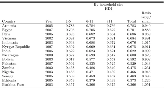
In this section, we present the results of the household-based HDI for our 15 countries. Table 1 shows the mean household-based HDI and its sub-components by country and also the outcomes for different approaches to cal-culate the household-based education index.28 HDI 1 refers to the approach where we simply drop the enrolment component and only rely on adult literacy, HDI 2 refers to the regression based approach to impute literacy and enrol-ment, and HDI 3 refers to the approach where we use the imputed gross school enrolment and years of education as the indicator of educational attainment.
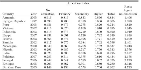
With respect to the different approaches to calculate the education index, the differences are shown in the last three columns of Table 1. We see small but significant differences between the regression based approach to impute literacy and enrolment and simply using the adult literacy rate to calculate the education index. Relying only on literacy and, thus, taking only one indicator of educational attainment into account, we potentially either underestimate or overestimate the education component compared to the approach where enrollment is also used, because the adult literacy rate is often either consid-erably lower or higher than the enrolment rates. This is illustrated in Table 2, which shows the descriptive statistics for all indicators. For example, in Ar-menia and Bolivia, literacy rates are much larger than enrolment rates which translates into a mich higher value for the education index relying only on literacy. Conversely, in the poorest African countries, including enrolment ra-tios leads to higher HDIs as they are higher than literacy levels. We find even larger level differences in the education index when we use years of education as the indicator of educational outcome instead of literacy. The education index based on years of schooling of adults aged 25 and older shows much lower outcomes than the other two approaches (see the last column of Table 1). This is because the mean values are considerably lower than the maximum of assumed 16 years of education achievable (see Table 2. These differences
28For all the results presented in this section, we do not provide any confidence intervals or significance tests between differences in the outcomes because of space limitations. Standard errors confidence intervals and significance test can be provided on request.
are than translated into an overall HDI which is significantly lower.29 This has an important implication considering a possible change in the calculation of the HDI for future Human Development Reports. The main question that arise here, is how one would compare the results of previous reports, because the values of the HDI are expected to be much higher. This would lead to a misleading interpretation of a decline in outcomes of human development.
However, besides differences in the level of the education index, the alter-native approaches to calculate the education index have almost no impact on the ranking of countries. Regardless of what approach chosen, the ranking between countries of the total HDI remains almost unchanged. This means for example, that Burkina Faso remains the country with the lowest value whereas Armenia remains the country with the highest outcome of the HDI. Only for the countries that are very close together in HDI values such as Viet-nam, Kyrgyz republic and India, the rankings change between these countries with respect to the underlying HDI alternative.
3.2 Overall results of the household based HDI, FLS, and Seth
measure
Table 1 reveals that Armenia shows the highest level in human development in our sample of countries with an HDI 2 value of 0.783 followed by Egypt (0.693), whereas the lowest value is found for two African countries, namely Burkina Faso (0.370) and Ethiopia (0.380). The high value of the HDI for Armenia is mainly driven by the high outcome in the life expectancy component (0.891) and the high outcome in the education component (0.835), both are also the highest in the sample. Although the GDP index is also high (0.623) it is not the highest value. Concerning levels in income, Egypt even shows a higher GDP index of 0.639. But since both the education index and the life expectancy index are considerably lower (0.802 and 0.639 respectively), the overall HDI is lower than for Armenia. This nicely illustrates the substitution possibilities between the three sub-components of the HDI. The higher education and life expectancy indices offset the relatively lower level of the GDP index. The same holds for Burkina Faso and Ethiopia, whereas the GDP index for Ethiopia is
29
Figures A2 and A3 provide the differences in the distribution between the alternative education indices and the alternative HDI outcomes.
slightly lower (0.356 compared to 0.367), Burkina Faso performs considerably lower in terms of education and life expectancy.
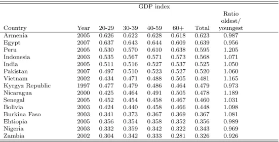
With respect to the question of what determines the variations in the overall outcomes, we find that variations in life expectancy outcomes are rela-tively low compared to the outcomes in education and the GDP component.30 Whereas the life expectancy index ranges from 0.507 (Nigeria) to 0.891 (Ar-menia), the GDP index ranges from 0.344 (Nigeria to 0.632 (Egypt) and the education index ranges from 0.204 (Burkina Faso) to 0.835 (Armenia), which is almost 4 times higher.
Table 3 provides the results for the household based HDI, the FLS and the Seth measure for several combinations of α and β; Table 4 provides the same information at the level of components of the HDI. We clearly see that as higher the inequality aversion parameter is as lower are the outcomes of the inequality adjusted FLS measure as well as its components. The percentage declines in the HDI (see 5) are particularly large for the low HDI countries suggesting that these countries are also the ones with the largest inequality across dimensions and across people (as we also see below). As shown in the tables, the rankings also change for some countries, particularly when inequality aversion is increased.31
We now turn to the analysis of outcomes of the HDI by different popu-lation subgroups and by household characteristics as well as to an analysis of inequality in human development. All results in the following section for the HDI are based on the regression based approach to estimate literacy and enrolment32.
3.3 Results by population subgroups and household
charac-teristics
In this subsection we provide the results of the outcome of the household-based HDI by different population subgroups and household characteristics. Table
30The same results are observable when looking at the official Human Development Re-ports.
31One should treat the higher levels of inequality aversion with some caution though. They are very sensitive to low values in the HDI components at the household level. Any measurement error in the imputation process leading to these low values for the components will have a large influence on the results.
32
6-11 present the HDI by HDI deciles, by income deciles, by education of the household head, by age of the household head, by the sex of the household head, and rural and urban areas. The respective tables for the subcomponents are found in the in the Appendix (Tables A5-A19).
Table 6 decompose the outcomes in human development by HDI quintiles itself. This provides us with a first sense of inequality in the outcome of human development. Table 6 shows large inequalities between the lowest and the highest HDI decile within countries. For example, in Nigeria the ratio of the highest to the lowest decile is 4.542. The ratio of the median to the highest and the lowest decile respectively further illustrates the inequality in human development.
The results of Table 6 suggest that inequality tend to be higher in settings where the level of human development is relatively low. The lower the values of the HDI (Table 1, the higher are the differences between the lowest and the highest HDI decile. This is plausible and reflects both the substance as well as construction of the HDI. An increase in the HDI is due to increases in the three components. As average education and life expectancy increases, the inequality within these components is declining due to the natural upper limits on achievements in these two dimensions. While there is no upper limit on incomes, due to the log transformation of incomes, inequality in incomes also falls as average incomes increase. This reflects the notion that there is a declining marginal impact of rising incomes on human development achieve-ments that are related to incomes (such as nutrition, housing, clothing, etc); as average incomes rise the disparity in these human development achieve-ments is correspondingly also held to fall.33 Despite this general trend, is it interesting to note that for similar levels of the overall HDI, the 10:1 decile ratio is quite different. For example, Peru has much higher HDI inequality than Egypt, Indonesia, or Vietnam; Nicaragua and Bolivia have much higher HDI inequality than Pakistan; and Nigeria has much higher HDI inequality than Senegal, Ethiopia, or Zambia.
This holds also when looking at the distribution of the HDI by income
33This is plausible to the extent that differences in nutritional status, essential access to housing and clothing are smaller in high HDI countries than in low HDI countries. See also Grimm et al. (2008) for further discussion.
decile, which is shown in Table 7. Also here, we observe a large inequality be-tween the lowest and the highest income quintile and also that this inequality is associated with lower levels of human development. Of course, the results for the income decile are not unexpected as the income component is inherent in the HDI. But this clear distributional pattern is also observed when the life expectancy index and especially the education index is analyzed by income decile (see Table A8-A10). In particular, we find the largest inequality be-tween the poorest and the richest income decile in the education component
34 Similar results for the outcomes of the HDI and its subcomponent by
in-come quintiles for some of the same countries (Indonesia, Vietnam, Bolivia, Zambia, and Burkina Faso) were also found in previous studies by Grimm et al. (2008, 2009), suggesting the use of slightly different methodological ap-proaches in that study does not seriously affect the results on inequality in human development.
The difference in distributions over the income quintiles and over the HDI quintiles needs a bit of discussion. When you look at the q10/q1 ratio for the HDI, it is larger than the same ratio for income deciles systematically for all countries (compare Tables 5 and 6). Note also that Table 13 shows that the Gini for the GDP index is in 8 (out of 13) cases larger than the Gini for the HDI. This suggests that the other components of the HDI are more equally distributed and that this distribution is not perfectly correlated with incomes. In this sense, the unconditional distribution of the HDI really shows something different than the HDI by income groups investigated in Grimm et al. (2008, 2009).
The same clear distributional pattern is found for education of the house-hold head. Househouse-holds, where the head has no education are considerably worse off in terms of the HDI than better educated households (Table 8. For example, Zambia shows a HDI that is almost twice as high for households where the household head has achieved higher education compared to house-holds where the head has no educational attainment at all (0.355 compared to 0.634). Again, the differentials are particularly large in Africa. A similar
34For example, in Burkina Faso the richest income decile show an education component that is more than 5 times higher than the poorest decile (Table A9).
pattern, but to lesser extent is found when looking at the outcomes in the HDI by the age of the household head. Although the inequality, is much lower than for other household characteristics, households with older household heads ex-perience, on average, a higher HDI than households with younger household heads.35
Quite surprisingly, no clear distributional pattern is found between be-tween male and female headed households (Tables 10). First, the differences are not very large, and, second, for some countries outcomes are higher for female headed households than for male headed households (e.g. Ethiopia) whereas the opposite is found for other countries (e.g. Egypt). It appears that female-headed households are a rather heterogeneous group that are not systematically worse off in terms of human development achievements than male-headed households (see also Chant 2008 and Marcoux, 1998 for related findings). Also for different household sizes no clear distributional pattern in the outcome of the HDI is found (Table 11). In some countries, smaller households show higher HDI outcomes than larger households, in some coun-tries again the opposite finds is found. However, in 10 from 15 councoun-tries larger households (more than 11 household members) show a lower HDI than smaller households (size 1-5).36
Table 12 shows the HDI by urban and rural areas. Also here, we find a clear trend. As expected, rural areas are worse off than urban areas with respect to human development. The differences are not as large compared to income deciles but they are always sizable. For example, in Nicaragua, the ratio between rural and urban areas in the HDI is 0.718. The differences tend to be larger in poorer countries, particularly in Africa and are smallest in Armenia, again driven to an important extent by low differentials in education and health there. And again, similar findings are also found for the sub-components of the HDI.37 The same differences are also found when looking at the alternative inequality adjusted HDI measure. In particular, Table 12
35
However, these results should be treated with caution, because they are also be driven by differences in the shares of households of the respective age ranges and thus the calculation are based in very different numbers of observation, For example, there are many more households with a household head aged between 20 and 29 than aged 60 years or older. See also Table A14-A16 for the results for the components of the HDI by the age of the household head.
36
See Table A18 for the results of the sub-components. 37See Table A19.
shows the results for the FLS and the Seth measure separately by urban and rural areas. We find that once a higher inequality aversion is introduced, the ratio between rural and urban outcomes also rises.
In Table 12, we extend this result and use the FLS approach to penalize for inequality within areas. In most places higher inequality in human devel-opment in rural areas generates a greater penalty for inequality there. But for extreme levels of inequality aversion, the finding can reverse. In Zambia, In-dia, and Egypt, the inequality-adjusted HDI for urban areas is lower than that for rural areas when alpha is set to -2, suggesting that there are some groups of urban residents with extremely low human development achievements.
To summarize the foregoing results, we identified significant differences between three alternatives ways to calculate education index. We found large differences in human development across HDI quintiles and income quintiles. The highest HDI quintile shows much higher outcomes in human development than the lowest HDI quintile for the HDI and with respect to all three sub-components of the HDI; the differential by income are somewhat smaller but still very large. Of the other population partitions, the largest differences are found for the education component. Furthermore, we found that human development in urban areas is considerably higher than in rural areas, revealing substantial differences in Africa. We also find that the age and education of the household head matters, but to a much smaller degree. Older households and households where the head has higher education achieve higher outcomes in the HDI. However, no clear picture for headship and household size emerges.
3.4 Inequality Measures and Decompositions
In addition to the household specific HDI, we also calculate standard inequal-ity measures. In particular, we calculated the Gini coefficient for the HDI and its subcomponents. In addition , we provide also the Theil index and Atkin-son index for the HDI and decompose the measure by within and between inequality for several household characteristics.
Table 13 shows the Gini coefficient, the Theil index and Atkinson index by countries for the HDI and its subcomponents. Although it is hard to interpret the absolute value of the Gini (see also below), we can compare the
outcome across countries and groups. Table 13 shows that higher values of inequality is found for those countries whose already have shown low levels of human development. For example, Burkina Faso is the country with the second highest Gini in the HDI (0.202) and at the same time is shows the lowest value of the HDI in our sample (see Table 1). On the other hand, Armenia (0.053) has the lowest value of the Gini coefficient for the HDI while at the same time it shows the second highest value of the HDI (see Table 1).
Why are the Gini coefficients relatively low compared to usual income Gini coefficients? Overall, the Gini coefficients for the HDI are considerably lower compared to the typical findings for income Gini coefficients. The reason for this relatively low inequality outcome is twofold. First, the main factor con-tributing to this low value is driven by the low level of inequality in the GDP index. The low values of the Gini coefficient for the GDP index nicely illus-trates how the log transformation of the GDP component reduces inequality. Table 13 provides also the Gini coefficient for the income, the GDP index with-out the log transformation of income and for the GDP index where the incomes were capped to the value of 40000. We can see that the Gini coefficients for the household per capita income show the expected values that nearly correspond to the official values of the countries taken from PovcalNet.38 The same holds for the GDP index without the log transformation and for the GDP index based on the capped household income per capita.39 This means, once we do the log transformation of the income component, we reduce artificially the potential inequality. This means, by using the log transformation, we face a trade-off between taking into account the diminishing rates of return of higher income on human development on the one hand and the focus of assessing the degree of inequality within a country or population subgroup on the other.
The second reason for relatively lower Gini coefficients in the HDI stems
38
The reason for these small differences is that the asset index distribution is less continu-ous than the income distribution. This means, for the imputation of the hcontinu-ousehold per capita income we do not take the whole income distribution, but rather draw from the distribution for the values of the asset index distribution.
39There is virtually no difference between the GDP index based in the capped and the uncapped income in our sample, because all these countries are relatively poor countries compared to OECD countries for which some countries like Norway exceeds a value of 40,000. In our case, only very few household show higher income values than the threshold resulting an similar values of the GDP index.