Optimal time of annuitization in the decumulation phase of a defined contribution pension scheme

(1)

ISSN: 2038-6087

Working Paper

Dipartimento di

Scienze Economiche

Università di Cassino

8/2010

Marina Di Giacinto

(1)

Bjarne Højgaard

(2)

Elena Vigna

(3)

(1) Università degli studi di Cassino - Italy

(2) Spar Nord Bank, Aalborg - Denmark

(3) Università degli studi di Torino, CeRP and Collegio Carlo Alberto - Italy

Optimal time of annuitization in the decumulation phase

of a defined contribution pension scheme

(2)

Dipartimento di Scienze Economiche

Università degli Studi di Cassino

Via S.Angelo Località Folcara, Cassino (FR) Tel. +39 0776 2994734 Email dipse@eco.unicas.it

(3)

Optimal time of annuitization in the decumulation

phase of a defined contribution pension scheme

∗

Marina Di Giacinto† Bjarne Højgaard‡ Elena Vigna§

Abstract

In this paper, we consider the problem of finding the optimal time of annuitization for a retiree of a defined contribution pension scheme having the possibility of choosing her own investment and consumption strategy. We exploit the model introduced by [7], who formulate the problem as a combined stochastic control and optimal stopping problem. They select a quadratic loss function that penalizes both the deviance of the running consumption rate from a desired consumption rate and the deviance of the final wealth at the time of annuitization from a desired target.

We make extensive numerical investigations to address relevant issues such as opti-mal annuitization time, size of final annuity upon annuitization, extent of improvement when annuitization is not immediate and comparison between optimal annuitization and immediate annuitization. We find that the optimal annuitization time depends on personal factors such as the retiree’s risk aversion and her subjective perception of remaining lifetime. It also depends on the financial market, via the Sharpe ratio of the risky asset. Optimal annuitization should occur a few years after retirement with high risk aversion, low Sharpe ratio and/or short remaining lifetime, and many years after retirement with low risk aversion, high Sharpe ratio and/or long remaining lifetime.

Moreover, we show rigorously that with typical values of the model’s parameters, a pension system where immediate annuitization is compulsory for all individuals is sub-optimal within this model. We measure the cost of sub-optimality in terms of loss of expected present value of consumption from retirement to death, and we find that the cost of sub-optimality, in relative terms, varies between 6% and 40%, depending on the risk aversion. This result gives an idea about the extent of loss in wealth suffered by a retiree who cannot choose programmed withdrawals, but is obliged to annuitize immediately on retirement all her wealth.

J.E.L. classification: D91, G11, G23, J26.

Keywords: Defined contribution pension scheme, decumulation phase, optimal an-nuitization time, cost of sub-optimality.

∗

The authors gratefully acknowledge financial support from Carefin - Bocconi Centre for Applied Re-search in Finance. We are also grateful to the anonymous referee for useful comments.

†

Dipartimento di Scienze Economiche, Universit`a degli studi di Cassino, Italy. Email: digiacinto at unicas.it

‡

Spar Nord Bank, Aalborg, Denmark. Email: bjh@sparnord.dk §

Dipartimento di Statistica e Matematica Applicata, Universit`a degli studi di Torino, CeRP and Collegio Carlo Alberto, Italy. Email: elena.vigna at econ.unito.it

(4)

1 Introduction

In defined contribution (DC) pension schemes, the financial risk is borne by the member: contributions are fixed in advance and the benefits provided by the scheme depend on the investment performance experienced during the active membership and on the price of the annuity at retirement, in the case that the benefits are given in the form of an annuity. Therefore, the financial risk can be split into two parts: investment risk, during the accumulation phase, and annuity risk, focused at retirement. In order to limit the annuity risk – which is the risk that high annuity prices (driven by low bond yields) at retirement can lead to a lower than expected pension income – in many schemes the member has the possibility of deferring the annuitization of the accumulated fund. This possibility consists of leaving the fund invested in financial assets as in the accumulation phase, and allows for periodic withdrawals by the pensioner, until annuitization occurs (if ever). In UK this option is named “income drawdown option”, in US the periodic withdrawals are called “phased withdrawals” or “programmed withdrawals”. There are a number of countries where programmed withdrawals are an option to retirees of DC schemes. These include Argentina, Australia, Brazil, Canada, Chile, Denmark, El Salvador, Japan, Peru,

(5)

UK. To the best of our knowledge, there are even substantially more countries where this option is not available. These include Austria, Bulgaria, Colombia, Germany, Hong Kong, India, Ireland, Italy, Luxembourg, Netherlands, Poland, Portugal, South Africa, Sweden, Switzerland. An exhaustive recent survey regarding the list of several forms of payment offered by pension schemes can be found in [2]. A pensioner who takes this option has three degrees of freedom:

1. she can decide what investment strategy to adopt in investing the fund at her dis-posal;

2. she can decide how much of the fund to withdraw at any time between retirement and ultimate annuitization (if any);

3. she can decide when to annuitize (if ever).

The first two choices represent a classical inter-temporal decision making problem, which can be dealt with using optimal control techniques in the typical [10] framework, whereas the third choice can be tackled by defining an optimal stopping time problem.

Examples of works dealing with these three choices via the formulation of a combined stochastic control and optimal stopping problem are [12], [15], [14] and [7].

Differently from the other mentioned papers, [7] solve the problem of optimal annu-itization in the presence of quadratic, target-depending loss functions. By so doing, the authors extend [5] and [6], where the optimal couple investment-consumption is found in the presence of quadratic loss function. Moreover, the authors leave scope for further re-search in many directions, both on the applicative side and on the theoretical one. In this paper, we address some of them, with particular emphasis on applications. Our extensions are twofold. Firstly, we carry out a broad sensitivity analysis of the results found by [7]. The main aim we have in mind is to provide a wide range of results regarding optimal annuitization time and consequent size of annuity in most common situations. Secondly, since optimality or not-optimality of immediate annuitization is shown to depend on the combination of the model parameters (i.e. risk aversion, market and mortality assump-tions), we show that in most cases a pension system where the only option available is immediate annuitization is sub-optimal. Moreover, we measure the cost of sub-optimality in terms of expected present value of consumption stream from retirement until death.

The reminder of the paper is organized as follows. Section 2 presents a review of the actuarial literature on the decumulation phase of DC pension funds. Section 3 presents the model exploited. Section 4 presents the performance analysis of results of the model. Section 5 shows the sub-optimality of immediate annuitization and measures its cost from the point of view of the member. Section 6 concludes.

2 Review of actuarial literature on decumulation phase

In the countries where the possibility of deferring ultimate annuitization is an option, the pensioner who takes this option can decide what investment strategy to adopt in investing the fund at her disposal, how much of the fund to withdraw at any time between retire-ment and ultimate annuitization, and when to annuitize. The evidence that the option

(6)

is actually taken by many pensioners is in apparent contrast with [17] fundamental work, according to which retirees should annuitize immediately at retirement. By addressing the three choices outlined above, the actuarial literature tries also to extend Yaari’s theorem and to give convincing explanations to the so-called “annuity puzzle”. Whereas the income drawdown option adds flexibility in the choices of the pensioner, and gives her the hope of being able to buy later on a better annuity than the one purchasable at retirement, the main drawback is that with self-annuitization the member bears the longevity risk, i.e. the risk of outliving her own assets. Therefore, another relevant issue that arises when the income drawdown option is chosen is the ruin probability, i.e. the probability that the pensioner runs out of money when she is still alive.

A number of authors have dealt with the problem of managing the financial resources of a pensioner after retirement and have investigated the alternatives available to a retiree other than immediate annuitization. It is not an easy task to classify properly the many papers that approach some or all of the four important issues outlined above, namely, investment and consumption strategies, optimal annuitization time, ruin probability, also because different methodologies have been adopted. Thus, we will first group them ac-cording to the topic addressed, then acac-cording to the methodology. Papers that address mainly the ruin probability are, e.g., [13] and [1]. Papers that explore different investment strategies and/or different consumption paths, possibly analyzing also the ruin issue are, e.g., [9], [16], [4], [5], [6]. Papers that add to their analysis also investigations on the optimal annuitization time are, e.g., [11], [8], [3], [12], [15] and [14]. An approach based on extensive simulations has been used by [9], [11], [1] and [3]. Stochastic optimal control has been applied by [5], [6], [12], [15] and [14].

In this paper we focus on the optimal time of annuitization. It is then important to review briefly the other contributions to this relevant topic. In [11] and [8], the basic idea is that since the annuity price is calculated with the riskfree rate, in the first years after retirement the equity risk premium pays more than the mortality credits (due to annuitants who die earlier than average); therefore in the first years after retirement the individual should invest and consume, and should annuitize when the mortality credits become so large that it becomes worthwhile annuitize (“do-it-yourself-and-then-switch” strategy). According to their simulations, in UK the maximum annuitization age of 75 (which is even 10 years greater than NRA1) is at least 5 years too low, and a Canadian female aged 65 has 90% probability of beating the interest rate return until the age of 80. [3] find that the optimal annuitization age is sensitive to the degree of risk aversion and varies from NRA (for very high risk aversion) to 79–80 (for very low risk aversion). [5] and [6] find that income drawdown option has to be preferred to immediate annuitization when risk aversion is not too high and the risky asset is sufficiently good compared to the riskfree one. [14] solve an optimization problem and find optimal investment/consumption strategies and optimal annuitization time using logarithmic utility function. They find that optimal annuitization age, which depends on the relative risk aversion and on the wealth status, is typically higher than 70. [7] solve a similar problem with quadratic loss functions. They find that optimal annuitization is mainly driven by risk profile of the retiree, level of the fund and market conditions and in some typical situations should occur 6–7 years

(7)

after retirement, but may occur also 10–15 years after it.

It is our opinion that the problem of finding optimal investment and consumption strategies and optimal annuitization time should be rigorously formulated as a combined stochastic control and optimal stopping problem. Up to our knowledge, in the literature this has been done only by [12], [15], [14], and [7]. While [12] minimize the probability of financial ruin, [15] finds optimal choices in a very general expected utility setting, dis-tinguishing between utility pre-annuitization and utility post-annuitization and selecting as a special case the power utility function, and [14] maximize expected utility of life-time consumption and bequest, with age-dependent force of mortality and power utility function. Differently from these papers, [7] solve the problem of optimal investment and consumption strategies as well as optimal annuitization time by selecting a quadratic loss function. We briefly present their model in the next section.

3 The model

A pensioner has a lump sum of size which can be invested either in a riskless asset paying interest at fixed rate or in a risky asset, whose price evolves randomly following a log-normal process. We assume that the remaining lifetime of the pensioner is exponentially distributed with constant force of mortality. The pensioner can choose the proportion of the fund to be invested in the risky asset and the withdrawal from the fund until to the time of annuitization. She is also able to select the time of eventual annuitization. The size of the annuity purchasable with sumxiskx, where k > r. If the amount of money in the fund is ever exhausted, no further investment or withdrawal is permitted, that means that occurrence of ruin is prevented by the model’s design.

We use this notation:

• y(t) is the proportion of the fund invested in the risky asset at timet;

• b(t)dt is the income withdrawn from the fund between time tand timet+dt.

• T is the time of annuitization;

• T0 is the time when the fund goes below 0;

• TD is the pensioner’s time of death, as measured from the time when the lump sum is received;

• x(t) is the size of the fund at time t(where t <min(T, TD, T0));

This model investigates the problem using y(·) and b(·) as control variables, and T as stopping time. The proportion invested in the fund, the income withdrawn, and the annuitization time are chosen in such a way as to minimize the following quadratic cost criterion Jb,y,T(x) =Ex " v Z τ 0 e−(ρ+δ)t(b0−b(t))2 dt+ we−(ρ+δ)τ ρ+δ (b1−kx(τ)) 2 # , (1) where:

(8)

• Ex(·) = E(·|x(0) = x), i.e. the expectation value is conditioned to the current size of the fund;

• τ = min(T, T0);

• v and w are positive weights which determine the relative importance in the cost criterion of the payment before and after annuitization, respectively;

• ρ is a subjective discount factor;

• δ is the force of mortality which is assumed to be constant;

• b0 is the income target before purchasing the annuity;

• b1 is the amount that represents the targeted income after eventual annuitization; • kis the amount of annuity which can be purchased with one unit of money. The intertemporal budget equation x is

dx(t) =

x(t) y(t)(λ−r) +r

−b(t)

dt+σx(t)y(t)dB(t),

where r is the instantaneous rate of return from the riskless investment and λ is the instantaneous rate of return from the risky investment with volatility σ. The standard Brownian motionB(·) is the source of uncertainty that represents market risk.

The amount b0, the income target until the annuity is purchased, will in many cases be equal tokx0, the size of the annuity which could have been purchased if the retiree had annuitized immediately on retirement. The processxevolves until either it is advantageous to annuitize or the fund falls to a negative value, in which case no further trading is permitted. The loss associated with annuitization when the level of the fund isx≥0, so that the annuity payskx per unit time, is

K(x) = w

ρ+δ(b1−kx)

2_. ₍₂₎

The ratio η = b1_b0 is a measure of risk propensity: the higher η, the higher the target, the lower the risk aversion and vice versa. Obviously the targeted annuity b1 is always assumed grater than income withdrawn b0, henceη >1.

Should the fund hit b1_k, the pensioner would be able to buy a lifetime annuity with income rate b1 and the penalty from that moment on would be null, which is what we expect to be.

Clearly, if the fund is equal to b1_k the optimal decision is to annuitize. However, the main novelty of the model is that optimal annuitization occurs also with a fund size x∗ lower than b1_k (see Section A.2). The intuition behind that is the following. When one reaches a certain level close enough to the desired target, it is better to stop the self-annuitization strategy and accept the low penalty given by (2), rather than keeping on investing and facing the risk of departing even more from the desired level.

The region where it is optimal the self annuitization strategy turns out to be U = (0, x∗)∪

b1 ,+∞

(9)

that in the optimal stopping theory terminology is called “continuation region”. The name of the region U is intuitive: if the wealth x is in the continuation region, then the loss paid in case of annuitization is higher than that paid in case of continuation of the optimization program, so that it is optimal to keep playing the game; vice versa, if one’s wealth is outside that region, then the loss paid in case of annuitization is lower than that paid playing the game, thus the game is over and the member annuitizes.

Quite remarkably, a complete solution of this optimal control model is given in [7]. While for a complete analysis of the mathematical model we refer to the original paper, for the reader’s convenience we provide a synthetic description of the optimal solution in appendix A.

4 The optimal annuitization time: performance analysis

In this section we carry out extensive simulations and scenario analysis in order to test the performance of the optimal exercise policies calibrating the model with realistic market parameters and mortality assumptions, and testing for different levels of risk aversion, i.e. subjective preferences.

4.1 Basic assumptions and scenario generation

We consider a male retiree aged 60 and time horizon equal toT = 30. In fact, accordingly to the existing actuarial literature (see section 2), ages of optimal annuitization range typically between 70 and 80, and only rarely up to 85-90. It is therefore reasonable to assume that if the pensioner has not annuitized at the age of 90, he will not do it later. His initial wealth is x0 = 100. The riskfree asset in each scenario will be chosen at 3%. For the annuity calculation, we make use of an Italian projected mortality table (RG48). This set of assumptions corresponds to an immediate annuity value equal to b0 = 6.22. The parameters of the problem are

r, λ, σ, δ, k, v, w, b1, ρ. (3)

In a realistic setting r,λ,σ characterize the investment opportunities and depend on the financial market,δ depends on the demographic assumptions, and kdepends on both the financial and demographic hypotheses.

Parameters that can be chosen are the weights given to penalty for running consump-tion, v, and to penalty for final annuitization, w, although it turns out that the relevant quantity is the ratio of these weights, w_v.Another parameter chosen by the retiree is the targeted level of annuity,b1, while it is reasonable to assume that the level of interim con-sumption b0 is given and depends on the size of the fund at retirement. A typical choice for b0 is the size of annuity purchasable at retirement with the initial fund x0. Thus, typically b1 is multiple ofb0, and the relevant quantity isη = b1_b0 >1.

A parameter that is somehow arbitrary and somehow given is ρ, the intertemporal discount factor: although subjective by its own nature, in typical situations cannot differ too much from the riskfree rate of returnr and in all our simulations it will be assumed

(10)

In this way the relevant quantity measuring the patience of the retiree for future events, the value of time, is given by the sum ρ+δ.

[7] show that, expectedly, what really counts in the applications, are some relevant ratios of these values, that are

β, b1

b0

, w

v, ρ+δ. (4)

This allows us in the following to fix some of the values (3) and change some others to get different values of the relevant quantities (4). In fact, they find that equal sign variations of the first three quantities and opposite sign variation of the fourth one produce equal qualitative variations to some relevant features of the problem solution (not reported here because too technical and not useful in this context). In particular, they find that everything else being equal, the ratio ₍_b1/kx∗ ₎, i.e. the width of the continuation region:

1. increases by increasingβ; 2. increases by increasing b1_b0; 3. increases by increasing w_v;

4. generally slightly decreases by increasingρ+δ.

Indeed, it is reasonable to accept that a high Sharpe ratio can well be coupled with low risk aversion, and also with high penalty in case of annuitization w.r.t. that paid in case of running consumption. Moreover, it is natural to expect that a low ρ+δ is consistent with a high w_v, because these choices are both led by high tolerance toward future income. And vice versa.

In a first set of simulations, here not reported, we let all the relevant quantities vary accordingly to the description. We have found out that the result do not differ very much when the ratio w_v increases. For this reason, we have finally fixed the ratio w_v equal to 1. Results have turned out to be more sensible to the choice ofr+δ that, as mentioned, measures the weight given to future and present flows, i.e. the time value of money for the retiree.

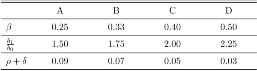
We fix four different scenarios, by starting with low values of the first two relevant quantities and high value of the third one, and then progressively augmenting the first two of them and reducing the third one, at the same time. The values of the relevant quantities of the four scenarios, which we call A, B, C, and D, are reported in Table 1.

Table 1: Value of parameters in scenarios A, B, C, D.

A B C D

β 0.25 0.33 0.40 0.50

b1

b0 1.50 1.75 2.00 2.25

(11)

Although, clearly, the set of combinations of different values of the relevant ratios is potentially unlimited, and the model can be run with different combinations, here we focus on these four scenarios, which we find representative for four different kinds of individuals:

• Scenario A would be suitable for individuals quite risk averse, who desire a pension target only 50% higher thanb0. They do not expose themselves too much to financial risk, and gain a small value of β on the market. These individuals strongly prefer current income to future income, probably due to a high estimate of the subjective mortality rate.

• Scenario B reports preferences for individuals moderately risk averse, who target a final pension 75% higher than b0. They find a β = 0.33 on the market, and give more weight to the present rather than the future.

• Scenario C would be suitable for individuals with low risk aversion, who aim to double their final annuity via programmed withdrawals. They are able to gain β = 40% on the financial market and give approximately the same importance to future and present income, taking into account also the mortality rate.

• Scenario D would be suitable to risk lovers, who aim to more than double the imme-diate annuityb0, and get a very high value ofβ on the market. They put substantial weight to future income, compared to present one, either due to low estimate of their own mortality rate or due to strict preference for the future.

4.2 Simulations results

For each scenario, we run 1000 Monte Carlo simulations for the risky asset. Across the four scenarios, we have fixed the 1000 trajectories of the Brownian motion. For each scenario, we provide the following:

• histogram with the distribution of the optimal annuitization time T∗, measured in years from retirement (Figures 1(a), 2(a), 3(a), 4(a));

• histogram with the distribution of the final annuityA∗achieved upon optimal annu-itization; the final annuityA∗ has been calculated each time through the actuarial fairness principle, using the RG48 mortality table and the interest rate r = 0.03; each time, the actual age of annuitization has been used, consistently with what would happen in the practice;

• distribution of optimal fund wealth evolution (via some percentiles);

• distribution of optimal consumption streamb∗, i.e. the optimal income withdrawal, between retirement and annuitization time (via some percentiles);

• distribution of optimal investment strategy y∗, i.e. portfolio quote invested in the risky asset, between retirement and annuitization time (via some percentiles);

• statistics of the optimal annuitization timeT∗ and of the size of annuityA∗ upon op-timal annuitization, with consequent comparison with that achievable on immediate annuitization (Tables 2, 4, 6, and 8);

(12)

• some relevant information relative to extreme cases, such as:

– probability of optimal annuitization within one year from retirement, Prob(T∗<1),

– probability of optimal annuitization after the time-frame considered, Prob(T∗ > 30),

– probability that the final annuityA∗ is lower or equal thanb1, Prob(A∗ ≤b1); – probability of negative optimal consumption, Prob(b∗ <0), and average time of negative consumption, given that there is negative consumption (Tables 3, 5, 7 and 9).

Here by Prob(E) we mean the frequency over the 1000 simulations of the event E. Summarizing, Figures 1(a), 1(b), 1(c), 1(d), 1(e) and Tables 2, 3 report results relative to scenario A; Figures 2(a), 2(b), 2(c), 2(d), 2(e) and Tables 4, 5 those relative to scenario B; Figures 3(a), 3(b), 3(c), 3(d), 3(e) and Tables 6, 7 those relative to scenario C; Figures 4(a), 4(b), 4(c), 4(d), 4(e) and Tables 8, 9 those relative to scenario D.

Remark 4.1 The statistics of optimal annuitization time and final annuity reported in Tables 2, 4, 6, and 8 are conditional on T∗ ≤30. When optimal annuitization does not occur within the 30-years time-frame,T∗ is set equal to 0, but its statistics is not reported into the mentioned Tables, and the same for the statistics of the final annuity. In a similar way, in Figures (a) and (b) of each scenario, that report the histograms of distribution of T∗ and final annuity A∗, the cases when optimal annuitization does not occur have not been reported. On the contrary, all other Figures (i.e. Figures (c), (d) and (e) for each scenario) report percentiles of optimal fund wealth and optimal policies over the 1000 scenarios. For this reason, there is no consistency in general between Tables 2, 4, 6, and 8 and Figures (c), (d) and (e).

Remark 4.2 Scenarios B, C and D are characterized by the same scale in all Figures, whereas scenario A differs from the others relatively to Figures 1(a) and 1(b). This is due to the much higher concentration of values around the mode of the distribution in scenario A than in the other scenarios.

4.2.1 Scenario A

The whole parameters’ value for this scenarios are the following

r= 0.03, λ= 0.06, σ = 0.12, δ = 0.06, k= 0.085, w= 1, v= 1, ρ= 0.03, b0= 6.22, b1= 9.33, x∗ = 104.24, that imply β = 0.25, b1 b0 = 1.50, ρ+δ= 0.09.

(13)

0 5 10 15 20 25 30 0 100 200 300 400 500 600 700 800

YEARS FROM RETIREMENT

FREQUENCY

ANNUITIZATION TIME

(a) Optimal annuitization time.

0 5 10 15 20 25 30 35 40 45 50 55 0 100 200 300 400 500 600 700 800 900 ANNUITY SIZE FREQUENCY FINAL ANNUITY (b) Annuity. 0 5 10 15 20 25 30 0 20 40 60 80 100 120 140 160 180 TIME OPTIMAL WEALTH

OPTIMAL FUND WEALTH

5° perc. 25° perc. 50° perc. 75° perc. 95° perc. x*

(c) Optimal fund wealth.

0 5 10 15 20 25 30 0 5 10 15 TIME b* OPTIMAL CONSUMPTION b₀ b₁ 5° perc 25° perc 50° perc 75° perc 95° perc (d) Optimal consumption. 0 5 10 15 20 25 30 0 0.2 0.4 0.6 0.8 1 1.2 1.4 1.6 1.8 TIME y*

OPTIMAL INVESTMENT STRATEGY

5° perc. 50° perc. 50° perc. 75° perc. 95° perc.

(e) Optimal amount invested in the risky asset.

(14)

Table 2: Statistics of the optimal annuitization time and the size of annuity in scenario A. annuitization time size of annuity mean 1.0312 6.8397 standard deviation 2.8087 1.2638 minimum 0.1923 6.4814 maximum 26.3077 25.9459 5th percentile 0.0192 6.4889 25th percentile 0.0769 6.5303 50th percentile 0.1731 6.5989 75th percentile 0.5962 6.7185 95th percentile 5.2173 7.5747

Table 3: Relevant information on extreme cases in scenario A.

Prob(T∗ <1) 77.00%

Prob(T∗ >30) 6.30%

Prob(A∗ ≥b1) 2.24%

Prob(b∗<0) 2.40%

Mean time of b∗ <0 (given b∗ <0) 4.40 yrs

From Figures 1(a), 1(b), 1(c), 1(d), 1(e) and from Tables 2 and 3 (recalling also Remark 4.1), we can gather the following information:

• the most striking feature that can be observed is the timing of optimal annuitization, T∗: in most of the cases,T∗ occurs only 1-2 years after retirement. In particular, in 77 cases out of 100 optimal annuitization occurs within one year from retirement;

• in 63 cases out of 1000 optimal annuitization does not occur within the time-frame of 30 years after retirement;

• the size of final annuity A∗ upon optimal annuitization is always higher than the pension achievable on immediate annuitization b0; however, the improvement does not seem to be particularly significant, since in 75% of the cases the final annuityA∗ lies between 6.48 and 6.71, vs b0 = 6.22. This is due to the fact that annuitization occurs too early and the price of annuity at that age is still too high, compared to the value ofkchosen, and this results into a low pension rate;

(15)

• in 98% of the cases the annuity value turns out to be lower thanb1. On the contrary, in very few cases (2.24%) the annuity value turns out to be higher than b1 = 9.33: this is due to annuitization occurring 20-25 years after retirement, when the old age of the pensioner pushes downwards the price of the annuity, leading to a high annuity value to be purchased with the wealth x∗;

• the results illustrated above are confirmed also by Figure 1(c), reporting the evolution of optimal fund wealth: the fund reaches the upper barrierx∗ in more than 95% of the cases immediately after retirement;

• the optimal consumption lies in most of the cases aboveb0, that is due to the fact that, as mentioned, after annuitization the optimal consumption is always (slightly) higher than b0; in 5% of the cases it lies always below b0, that is due to the cases in which optimal annuitization occurs later, coupled with the fact that optimal consumption is bound by the model to be lower thanb0;

• the optimal investment strategy is 0 after optimal annuitization, that explains why in Figure 1(e) most of the percentiles collapse to 0 a few years after retirement. The trajectories that survive after 5 years post retirement seem to be very risky, with approximately 150% of the wealth invested in the risky asset for the whole time-frame of 30 years;

• optimal negative consumption occurs in 24 cases out of 1000, and on average con-sumption remain negative for 4 years.

4.2.2 Scenario B

r= 0.03, λ= 0.08, σ = 0.15, δ = 0.04, k= 0.085, w= 1, v= 1, ρ= 0.03, b0= 6.22, b1= 10.89, x∗ = 126.78, that imply β = 0.33, b1 b0 = 1.75, ρ+δ= 0.07.

(16)

0 5 10 15 20 25 30 0 20 40 60 80 100 120 140 160 180 200

FREQUENCY

ANNUITIZATION TIME

0 5 10 15 20 25 30 35 40 45 50 55 0 50 100 150 200 250 300 350 ANNUITY SIZE FREQUENCY FINAL ANNUITY (b) Annuity. 0 5 10 15 20 25 30 0 20 40 60 80 100 120 140 160 180 TIME OPTIMAL WEALTH

OPTIMAL FUND WEALTH

5° perc. 25° perc. 50° perc. 75° perc. 95° perc. x* (c) Optimal wealth. 0 5 10 15 20 25 30 0 5 10 15 TIME b* OPTIMAL CONSUMPTION b₀ b₁ 5° perc 25° perc 50° perc 75° perc 95° perc (d) Optimal consumption. 0 5 10 15 20 25 30 0 0.2 0.4 0.6 0.8 1 1.2 1.4 1.6 1.8 TIME y*

(17)

Table 4: Statistics of the optimal annuitization time, size of annuity deriving from scenario B. annuitization time size of annuity mean 8.1532 11.6771 standard deviation 7.2171 5.9555 minimum 0.5385 7.8838 maximum 29.9231 39.3369 5th percentile 1.2500 8.1209 25th percentile 2.6346 8.4399 50th percentile 5.4423 9.2200 75th percentile 11.6539 11.7757 95th percentile 24.3798 25.7227

Table 5: Relevant information on extreme cases in scenario B.

Prob(T∗ <1) 2.20%

Prob(T∗ >30) 25.30%

Prob(A∗ ≥b1) 29.58%

Prob(b∗<0) 5.30%

From Figures 2(a), 2(b), 2(c), 2(d), 2(e) and from Tables 4 and 5 (recalling Remark 4.1) we can gather the following information:

• the timing of optimal annuitization, T∗ is much more spread out than in scenario A: on average,T∗ occurs 8 years after retirement, and in 50% of the cases it occurs after 5 years. In only 2 cases out of 100 optimal annuitization occurs within one year from retirement and in 25% of the cases it occurs at a date later than 11 years after retirement;

• in 253 cases out of 1000 optimal annuitization does not occur within the time-frame of 30 years after retirement;

• the size of final annuity A∗ upon optimal annuitization is always higher than the pension achievable on immediate annuitization b0; this time, the improvement is more significant than in scenario A, since in 75% of the cases the final annuity A∗ lies between 7.88 and 11.77, vs b0 = 6.22. This is due to the fact that now optimal

(18)

annuitization occurs at a later age than in scenario A and the price of annuity at that age is sufficiently low to guarantee a mode than adequate improvement in the pension rate;

• in 30% of the cases the annuity value turns out to be higher than b1 = 10.89: as before, this is due to annuitization occurring 15-25 years after retirement, when the relatively old age of the pensioner pushes downwards the price of the annuity, leading to a high annuity value to be purchased with the wealth x∗;

• Figure 2(c) shows that the fund does not reach the upper barrier x∗ in slightly more than 25% of the cases, whereas in 500 cases out of 1000 x∗ is reached within approximately 8 years;

• clearly the optimal consumption lies below b0 in slightly more than 250 cases out of 1000, due to the fact that optimal annuitization does not occur. However, when optimal annuitization does occur the pension rate is sensibly higher thanb0 and in slightly less than 250 cases out of 1000 it is higher than b1;

• the optimal investment strategy is bounded between 0 and 1 in slightly more than 75% of the cases; short-selling occurs in less than 20% of the cases, but in 50 cases out of 1000 strategies can be very risky, with riskiness increasing with time and reaching in 5% of the cases 300% of the fund invested in the risky asset;

• optimal negative consumption occurs in 53 cases out of 1000, and on average con-sumption remains negative for 2.8 years.

4.2.3 Scenario C

r= 0.03, λ= 0.102 σ= 0.18, δ= 0.02, k= 0.085, w= 1, v= 1, ρ= 0.03, b0= 6.22, b1= 12.44, x∗ = 146.12, that imply β= 0.40, b1 b0 = 2, ρ+δ= 0.05.

(19)

0 5 10 15 20 25 30 0 20 40 60 80 100 120 140 160 180 200

FREQUENCY

ANNUITIZATION TIME

OPTIMAL FUND WEALTH

(20)

Table 6: Statistics of the optimal annuitization time, size of annuity in scenario C. annuitization time size of annuity mean 14.1807 18.0114 standard deviation 7.3754 28.8639 minimum 2.0000 9.6208 maximum 30.0000 49.1624 5th percentile 4.3933 10.2426 25th percentile 7.8798 11.4980 50th percentile 12.7885 14.1752 75th percentile 19.7067 20.8759 95th percentile 27.5106 38.0239

Table 7: Relevant information on extreme cases in scenario C.

Prob(T∗ <1) 0.00%

Prob(T∗ >30) 34.10%

Prob(A∗ ≥b1) 63.13%

Prob(b∗<0) 3.20%

From Figures 3(a), 3(b), 3(c), 3(d), 3(e) and from Tables 6 and 7 (recalling Remark 4.1we can gather the following information:

• the distribution of optimal annuitization, T∗, has more or less the same dispersion than in scenario B, but the mean is much higher: on averageT∗occurs 14 years after retirement, and in 50% of the cases it occurs after 13 years. Optimal annuitization never occurs within one year from retirement and the minimum T∗ is equal to 2 years. In 25% of the cases it occurs at a date later than 20 years after retirement;

• in 341 cases out of 1000 optimal annuitization does not occur within the time-frame of 30 years after retirement; this too high percentage of individuals not annuitizing before age 90 is the price to be paid when the target aimed is chosen to be very high;

• the size of final annuityA∗ upon optimal annuitization is always significantly higher than the pension achievable on immediate annuitization b0; the improvement with respect tob0is now remarkable: in 75% of the cases the final annuityA∗ lies between

(21)

higher than before and that optimal annuitization occurs at a much later age, with consequent very low price of the annuity;

• in 63% of the cases the annuity value turns out to be higher than b1 = 12.44: as before, this is due to annuitization occurring 15-25 years after retirement, when the relatively old age of the pensioner pushes downwards the price of the annuity, leading to a high annuity value to be purchased with the wealth x∗;

• Figure 3(c) shows that the fund does not reach the upper barrier x∗ in more than 25% of the cases, whereas in 500 cases out of 1000x∗ is reached within approximately 20 years;

• the optimal consumption lies below b0 in approximately 250 cases out of 1000, due to the fact that optimal annuitization does not occur. However, when optimal annu-itization does occur the pension rate is sensibly higher thanb0, being almost always higher than 10, and in slightly less than 500 cases out of 1000 it is higher thanb1; • the optimal investment strategy is bounded between 0 and 1 in slightly more than

75% of the cases; short-selling occurs in less than 20% of the cases, but in 50 cases out of 1000 strategies can be risky, reaching in 5% of the cases 150% of the fund invested in the risky asset; therefore, strategies seem to be less risky than in scenario B;

• optimal negative consumption occurs in 32 cases out of 1000, and on average con-sumption remains negative for 2 years.

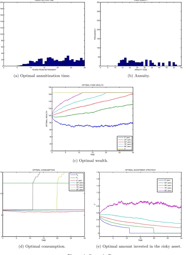
4.2.4 Scenario D

r= 0.03, λ= 0.13 σ= 0.20, δ = 0.005, k= 0.085, w= 1, v= 1, ρ= 0.03, b0= 6.22, b1= 14.00, x∗ = 164.70, that imply β = 0.50, b1 b0 = 2.25, ρ+δ= 0.035.

(22)

0 5 10 15 20 25 30 0 20 40 60 80 100 120 140 160 180 200

FREQUENCY

ANNUITIZATION TIME

OPTIMAL FUND WEALTH

(23)

Table 8: Statistics of the optimal annuitization time, size of annuity in scenario D. annuitization time size of annuity mean 19.6263 26.8969 standard deviation 6.1493 10.9322 minimum 5.3462 11.9479 maximum 30.0000 54.8383 5th percentile 9.6769 13.8827 25th percentile 14.1923 17.5521 50th percentile 19.5962 23.5142 75th percentile 24.6250 33.4876 95th percentile 29.0558 50.3146

Table 9: Relevant information on extreme cases in scenario D.

Prob(T∗ <1) 0.00%

Prob(T∗ >30) 50.09%

Prob(A∗ ≥b1) 93.48%

Prob(b∗<0) 1.10%

From Figures 4(a), 4(b), 4(c), 4(d), 4(e) and from Tables 8 and 9 (recalling Remark 4.1) we can gather the following information:

• the most striking feature is the probability that optimal annuitization does not occur in the 30 years time-frame: indeed, it is as high as 50.90%. In section 5 we will argue that with such a high probability of failure to annuitizing in a reasonable time horizon, this model should not be used.

• whenT∗ <30, it occurs on average after 19 years from retirement, with a moderately high dispersion; in 70% of the cases it occurs between 10 and 25 years from retire-ment. Moreover, optimal annuitization never occurs within 5 years from retireretire-ment. In 25% of the cases it occurs at a date later than 25 years after retirement;

• the size of final annuity A∗ upon optimal annuitization is dramatically higher than the pension achievable on immediate annuitization b0: in case of optimal annuiti-zation the minimum pension rate achieved is 11.94, that is almost the double than b0= 6.22, and the size of annuity between the fifth and the seventy-fifth percentiles

(24)

ranges between 14 and 33, while in 25% of the cases it ranges between 33 and 50. This is mainly due to the too high selected b1, that leads to an extremely high value ofx∗: in the most favorable scenarios, when x∗ is reached, the annuity size is extremely high;

• the results on the size of annuity are confirmed also by the fact that in 93% of the cases the annuity value turns out to be higher thanb1 = 14;

• as expected, Figure 3(c) shows that the fund does not reach the upper barrierx∗ in slightly more than 50% of the cases, whereas in 250 cases out of 1000x∗ is reached within approximately 20 years and in 50 cases out of 1000 x∗ is reached within approximately 12 years;

• Figure 4(e) shows that the optimal consumption in 50% of the cases lies always below b0: in the remaining 50% of the cases percentiles increase sharply due to optimal annuitization that leads to optimal consumption in most cases well aboveb1; • a somewhat unexpected feature is that the optimal investment strategy in 95% of

the cases is always bounded between 0 and 1; therefore, strategies seem to be more stable than in the other scenarios;

• optimal negative consumption occurs in 11 cases out of 1000, and on average con-sumption remains negative for 2 years.

4.3 Sensitivity analysis with different k

A relevant feature of the model is that the conversion coefficientkis fixed over time. This is mainly due to the much harder nature of the problem, from the mathematical point of view, if a more appropriate time-dependent k were to be chosen. The individual is then bound to choose her ownk at retirement. Different considerations affect this choice. Typically,k should be linked to the sum of the two factorsδs+ρ.

In fact,kshould be somehow linked to the expected subjective remaining lifetime, that is driven byδs: the lowerδs, the longer the individual expects to live, the lowerk, that in turn leads to a higher wealth target b1_k. This is consistent with the fact that the individual can wait until she obtains the desired annuity, because she thinks she will live long enough to enjoy it. On the other hand, individuals with short subjective remaining lifetime (i.e. high δs) would not find convenient to aim to a too high annuity target, because they would face the risk of dying before having the possibility of receiving it. So, they will choose a high k, leading to a low wealth target b1_k, that triggers optimal annuitization in a reasonable time-frame.

A similar relationship linkskand the tolerance towards future income, that is linked to ρ: the smaller ρ, the higher the tolerance towards future, the more willing the individual is to wait until the desired annuity can be achieved, so the lower the choice ofk. And vice versa.

It is therefore useful to make a sensitivity analysis also with respect to the factor k. We have selected the scenario B and run the simulations with the two additional values k= 0.08 and k= 0.09. We would like to remark that all the parameters of the model are

(25)

equal across scenarios, exceptk. This seems to be relevant because it allows for consistent comparisons in the presence of the same financial market conditions.

For brevity of exposition, we report here only a comparative table (Table 10) that summarizes some statistics of optimal annuitization time and final annuity and reports relevant information on extreme cases for the 3 scenarios, and the histograms reporting the distribution of optimal annuitization time and the final annuity. All other Figures (relative to optimal policies and optimal wealth) as well as the Table reporting the percentiles of these distributions, available from the authors upon request, are not reported because they do not add valuable information. Figures 5(a), 5(c), 5(e) report the histograms of the optimal annuitization time, Figures 5(b), 5(d), 5(f) report the histograms of the size of final annuity upon optimal annuitization.

(26)

0 5 10 15 20 25 30 0 20 40 60 80 100 120 140 160 180 200

FREQUENCY

ANNUITIZATION TIME

(a) Scenario B withk= 0.080.

0 5 10 15 20 25 30 35 40 45 50 55 0 50 100 150 200 250 300 350 400 450 500 550 ANNUITY SIZE FREQUENCY FINAL ANNUITY (b) Scenario B withk= 0.080. 0 5 10 15 20 25 30 0 20 40 60 80 100 120 140 160 180 200

FREQUENCY ANNUITIZATION TIME (c) Scenario B withk= 0.085. 0 5 10 15 20 25 30 35 40 45 50 55 0 50 100 150 200 250 300 350 400 450 500 550 ANNUITY SIZE FREQUENCY FINAL ANNUITY (d) Scenario B withk= 0.085. 0 5 10 15 20 25 30 0 20 40 60 80 100 120 140 160 180 200

FREQUENCY

ANNUITIZATION TIME

(e) Scenario B withk= 0.090.

0 5 10 15 20 25 30 35 40 45 50 55 0 50 100 150 200 250 300 350 400 450 500 550 ANNUITY SIZE FREQUENCY FINAL ANNUITY (f) Scenario B withk= 0.090.

Figure 5: The optimal annuitization time and final annuity in scenarios B with k = 0.080,0.085,0.090.

(27)

Table 10: Relevant information in scenario B, withk= 0.080,0.085,0.090. k= 0.080 k= 0.085 k= 0.090 meanT∗ 11.0091 8.1532 5.7240 standard deviationT∗ 7.6160 7.2171 6.4095 meanA∗ 14.3330 11.6771 9.6840 standard deviationA∗ 7.4077 5.9556 4.2089 Prob(T∗<1) 0.00% 2.20% 13.20% Prob(T∗>30) 37.10% 25.30% 16.50% Prob(A∗ ≥b1) 52.30% 29.58% 17.00% Prob(b∗ <0) 5.50% 5.30% 4.60%

Mean time of b∗<0 (givenb∗ <0) 2.69 yrs 2.84 yrs 3.10 yrs

From Figures 5(a), 5(b), 5(c), 5(d), 5(e) and Table 10 we can gather the following information:

• clearly, in all cases, results f the case k= 0.085 fall between those for k= 0.08 and k= 0.09, so we will focus on commenting the extreme values only;

• as expected, the annuitization time is longer when k is smaller, reflecting the fact that small k leads to high targeted wealth, and therefore longer achievement time, also considering the feature that here all parameters of the model (included the financial market) are equal across scenarios;

• in particular, with k= 0.09 it turns out optimal to annuitize within one year from retirement in 13.20% of the cases, never with k= 0.08;

• on the other hand optimal annuitization does not occur within the 30 years’ time-frame in 371 cases out of 1000 when k = 0.08, in only 165 cases out of 1000 when k= 0.09;

• expectedly, mean and standard deviation of the final annuity are low withk= 0.09: this is the effect of more cautious optimal investment strategies (here not reported) that are the caused by a lower targeted wealth;

• on the contrary, there is high dispersion of the final annuity when k = 0.08, that produces on the one side a fairly high probability of exceeding b1, on the other side a high probability of not annuitization within 30 years;

• curiously, the dispersion of the optimal annuitization time does not vary very much across scenarios.

(28)

5 Sub-optimality of immediate annuitization

In this section, we show that in the majority of cases, a pension system where full or partial annuitization is compulsory immediately at retirement is sub-optimal. The extent and the cost of sub-optimality is measured by the comparison between expected present value (EP V) of consumption stream from retirement up to death in the two cases of immediate annuitization (EP VIA) and optimal annuitization (EP VOA). The ambitious aim behind this evidence would be to suggest appropriate adjustments to the existing legislation in order to increase flexibility in choosing benefits after retirement, and allow optimal choices for pensioners.

5.1 A rigorous criterion for optimality of immediate annuitization

In the model outline above, the sub-optimality of immediate annuitization turns out to be easy to check. An easy and efficient criterion to this aim is provided by the following theorem.

Theorem 5.1 In the model outlined in Section 3, for any initial wealth x∈h0,b1_ki, it is optimal to annuitize immediately at retirement if and only if

φ≤2rDk b1 , (5) where D= b0_r −b1_k and φ=ρ+δ+β2−2r+k2_v₍_ρw₊_δ₎. Proof (⇐) See [7], Lemma 7. (⇒) If T∗ = 0 for all x ∈ h0,b1_k i

, then V(x) = K(x), where V and K respectively are given by (6) and (2). Therefore,

LK(x) = inf b,y v(b0−b)2−(ρ+δ)K+ [−b+ (λ+r)yx+rx]K0+ 1 2σ 2_y2_x2_K00 ≥0,

for all x∈h0,b1_ki. This, in turn implies that given the set U0 defined as

U0 ={x∈R : LK(x)<0}, we have U0∩ 0,b1 k =∅.

On the other hand, it is easy to show (see [7]) that ifφ >2rD_b1k, thenU0∩

h 0,b1_k i 6 =∅. Then, necessarily φ≤2rDk b1 .

(29)

We believe that the practical implications of Theorem 5.1 are really worth exploring. In a pension system where immediate full or partial annuitization is the only option, which is the current situation in Italy for instance, the lack of flexibility in choosing timing of annuitization can be shown to be sub-optimal in a relatively immediate way.

We will show practical implications of the Theorem in two ways:

1. we check sub-optimality in the four scenarios fixed in the previous section. These scenarios clearly do not exhaust all possible existing situations, but are by no means representative of many typical ones;

2. in the six scenarios chosen, we calculate the cost of being sub-optimal. We do this by calculating and comparing the expected present value of consumption stream from retirement up to death in the two cases of immediate annuitization and optimal annuitization.

5.2 Sub-optimality of immediate annuitization: application of the crite-rion

Straight application of the definitions allows us to check that, as expected, in the four scenarios chosen the criterion (5) is not satisfied. Therefore, Theorem 5.1 indicates that it is not true thatfor each initial fund x(0) the optimal annuitization time is T∗ = 0. This does not mean that T∗ = 0 is never optimal, for there are cases in which φ > 2krD/b1 and x(0) stays in the stopping region, leading to T∗ = 0. This happens, for instance, if one chooses a too low value of b1_b0: results of simulations not reported here indicate that this ratio cannot be too low, if the potentialities of programmed withdrawals want to be completely exploited. For this reason, in the most conservative scenario (scenario A) we have selected b1_b0 = 1.5. With lower values of b1_b0 it either happens that the initial wealth lies in the stopping region betweenx∗ and b1_k that implies that immediate annuitization is indeed optimal or, even worse from the modeling point of view, is higher than b1_k, rendering the problem not interesting.

Thus, based on Theorem 5.1 and on current realistic values for the model’s parameters, we argue that if the preferences and needs of pensioners can be represented by the model exploited, then a system where immediate annuitization is compulsory and programmed withdrawals are not an option is bound to be sub-optimal. Clearly, accordingly to the Theorem and to the results not shown here, immediate annuitization turns out to be optimal within this model for retirees with high risk aversion and ratio b1_b0 lower than 1.50. However, taken as a whole a pension system that imposes compulsory immediate annuitization and lack of flexibility for the entire universe of retirees turns out to be sub-optimal. It is indeed clear from the analysis performed in the previous section, that programmed withdrawals allow the pensioner to exploit the potentialities of the financial market and to succeed most of the times in achieving a final annuity higher than that purchasable at retirement. The extent of improvement clearly depends on the risk aversion and therefore on the scenario selected. In scenario A, the pensioner is better off in almost all cases, but the improvement in pension rate is modest in entity. On the contrary, in scenarios C and D, characterized by low risk aversion, the increase in the pension rate is significantly higher, but the frequency of failure to annuitize within 30 years is high.

(30)

The next section is devoted to measuring the extent of sub-optimality for the single individual in the four scenarios selected previously.

5.3 Sub-optimality of immediate annuitization: cost of sub-optimality

In this section, we measure the cost of sub-optimality in terms of loss of expected present value (EP V) of consumption stream from retirement up to death. In particular, we calcu-lateEP V in the two cases of optimal annuitization (EP VOA) and immediate annuitization (EP VIA) and make the difference. Henceforth, we will call the differenceEP VOA−EP VIA

cost of sub-optimality,orsub-optimality cost (SC). In other words, SC =EP VOA−EP VOA= cost of sub-optimality.

It is important to underline that we focus only on those trajectories for which optimal annuitization has actually occurred between retirement and the time-horizon of 30 years. The trajectories where the optimal fund fails to reach x∗ within the time-frame of 30 years have been assigned a 0 value to the SC, because the model does not require a finite time-horizon and, more importantly, because optimal annuitization at a later age would produce different results in terms of SC. Assignment ofSC = 0 to all trajectories where optimal annuitization does not occur is the explanation for a bar around 0 in the histograms. However, in the statistics of SC (Table 11) we will not consider the zeroes and will present the statistics only for the relevant cases in whichT∗ <30.

In each scenario and for each trajectory, the EP V of consumption stream has been calculated according to actuarial principles with the interest rater for the financial basis, and with the mortality table RG48 for the demographic basis. For the immediate annu-itization option the flow to be discounted is equal to b0 at any time from retirement up until age 110. For the optimal annuitization case, the flow to be discounted is equal to the optimal consumption from retirement until age of optimal annuitizationT∗, to the actual pension rate achieved from that time up to age 110.

To better give an idea of the improvement that can be achieved in case of optimal annuitization, we define a new quantity, called the ”Relative SC”. this is defined as the ratio between the average cost of sub-optimality and theEP V of immediate annuitization:

Relative SC= Average(SC) EP VIA

.

This quantity indicates by how much on average and in percentage the pensioner can increase her reward (measured in terms ofEP V of consumption) by adopting programmed withdrawals with respect to immediate annuitization.

Figures 6(a), 6(b), 6(c), 6(d) report the histograms of the distribution of SC in sce-narios A, B, C and D, respectively. Figures 7(a), 7(b), 7(c) report the histograms of the distribution of SC in scenarios B (k=0.08), B(k=0.085) and B(k=0.09), respectively.

(31)

−10000 −500 0 500 1000 1500 2000 2500 3000 3500 50 100 150 200 250 300 350 400 450 500 550 EPVOA − EPVIA FREQUENCY

COST OF SUBOPTIMALITY GIVEN T* ≤ 30

(a) Scenario A. −10000 −500 0 500 1000 1500 2000 2500 3000 3500 50 100 150 200 250 300 350 400 450 500 550 EPVOA − EPVIA FREQUENCY

(b) Scenario B. −10000 −500 0 500 1000 1500 2000 2500 3000 3500 50 100 150 200 250 300 350 400 450 500 550 EPV_OA − EPV_IA FREQUENCY

(c) Scenario C. −10000 −500 0 500 1000 1500 2000 2500 3000 3500 50 100 150 200 250 300 350 400 450 500 550 EPV_OA − EPV_IA FREQUENCY

(d) Scenario D.

Figure 6: The sub-optimality cost deriving from scenarios A, B withk= 0.085, C and D respectively.

(32)

−10000 −500 0 500 1000 1500 2000 2500 3000 3500 50 100 150 200 250 300 350 400 450 500 550 EPV_OA − EPV_IA FREQUENCY

(a) Scenario B withk= 0.080.

−10000 −500 0 500 1000 1500 2000 2500 3000 3500 50 100 150 200 250 300 350 400 450 500 550 EPV_OA − EPV_IA FREQUENCY

(b) Scenario B withk= 0.085. −10000 −500 0 500 1000 1500 2000 2500 3000 3500 50 100 150 200 250 300 350 400 450 500 550 EPV_OA − EPV_IA FREQUENCY

(c) Scenario B withk= 0.090.

(33)

Table 11 reports for each scenario:

• as a reminder, the probability that optimal annuitization occurs in the time-frame (i.e. the number of trajectories considered in this analysis for each scenario divided by 1000);

• some statistic of the cost of sub-optimality across the six scenarios generated so far;

• the probability that the cost of sub-optimality is positive;

(34)

T able 11: Statistics of the cost of sub-optimalit y deriving from all scenarios. Scenario A Scenario B k = 0 . 085 Scenario B k = 0 . 080 Scenario B k = 0 . 090 Scenario C Scenario D Prob( T ∗ > 30) 6 . 30% 25 . 30% 37 . 10% 16 . 50% 34 . 10% 50 . 90% Prob( S C > 0) 93 . 60% 73 . 50% 61 . 80% 82 . 90% 65 . 00% 49 . 00% Relativ e S C 6.62% 28.91% 34.23% 22.68% 38.80% 38.82% mean 338.9556 1,479.9263 1,752.2192 1,160.7481 1,985.7943 1,987.0308 standard deviation 134.4206 378.5419 521.0240 254.1689 700.8871 935.0963 minim um -514.0536 -726.6107 -452.7231 -462.7413 -499.4168 -16.5548 maxim um 938.7281 1, 988.1095 2,252.7074 1,653.1588 2,697.1238 3,340.5489 5th p ercen tile 214.8806 603.5453 350.8363 842.9542 352.3035 301.9541 25th p ercen tile 248.7041 1,451.6475 1,791.7037 1,058.2206 1,724.5226 1,254.0524 50th p ercen tile 303.6802 1,568.8207 1,947.4271 1,177.7094 2,350.9992 2,200.6371 75th p ercen tile 383.6738 1,675.8389 2,040.0014 1,317.1619 2,458.8257 2,841.1091 95th p ercen tile 642.5026 1,789.9402 2,128.3859 1,465.6558 2,561.7912 3,183.1867

(35)

From Figures 6(a), 6(b), 6(c), 6(d), Figures 7(a), 7(b), 7(c), 7(d) and Table 11 we can gather the following information:

• considering that the sum of the number of cases in which optimal annuitization does not occur and number of cases characterized by SC >0 (sum of the first two lines of table 11) is almost approximately 99%, for each scenario we find that in all but 10 cases in which optimal annuitization occurs, the sub-optimality cost is positive, meaning that the pensioner is better off when programmed withdrawals are adopted;

• the few cases when optimal annuitization does occur butSC <0 are motivated by the fact that the dynamic programming approach minimizes the expected loss (or maximizes expected utility) and fails to capture very rare unfavorable scenarios (e.g. extreme events);

• the extent of improvement withOA (or the extent of loss with IA) is measured by the Relative SC, in the third line of the Table: it amounts to only 7% for scenario A, to 29% for scenario B, 39% for scenarios C and D. As expected, the margin of improvement increases when risk aversion of the individual decreases. This is highlighted also by the comparison of the Relative SC with different k: higher k produces smaller Relative SC, that increases whenk reduces;

• the probability of failure in achievingx∗, as was already observed elsewhere, sharply increases when aiming to higher targeted pension rate.

Table 12 below summarizes all relevant results for the six scenarios considered in this analysis.

(36)

T able 12: Statistics of all relev an t quan tities in all sce n arios. Scenario A Scenario B k = 0 . 085 Scenario B k = 0 . 080 Scenario B k = 0 . 090 Scenario C Scenario D mean S C 338.9556 1,479.9263 1,752.2192 1,160.7481 1,985.7943 1,987.0308 standard deviation S C 134.4206 378.5419 521.0240 254.1689 700.8871 935.0963 Prob( S C > 0) 93.60% 73.50% 61.80% 82. 90% 65.00% 49.00% Relativ e S C 6.62% 28.91% 34.23% 22.68% 38.80% 38.82% mean T ∗ 1.031237 8.153151 11.009111 5.723975 14.180664 19.626312 standard deviation T ∗ 2.808690 7.217116 7.6160384 6.409536 7.375429 6.1492750 Prob( T ∗ < 1) 77.00% 2.20% 0.00% 13.20% 0.00% 0.00% Prob( T ∗ > 30) 6.30% 25.30% 37.10% 16.50% 34.10% 50.90% mean 6.839652 11.677057 14.332950 9.684013 18.011367 26.896878 standard deviation A ∗ 1.263751 5.955538 7.407654 4.208856 28.863906 10.932189 Prob( A ∗ ≥ b1 ) 0.022412 0.295850 0.523052 0.170060 0.631259 0.934827

(37)

Table 12 allows a broad comparison among all scenarios regarding all types of quantities analyzed throughout the paper. Let us recall that the scenarios A, B, C and D are descriptive of different risk aversion attitudes, with the A scenario representing the highest and the D scenario reporting the lowest. The scenarios B with differentkindicate different ways of discounting future income and considering one own’s remaining lifetime: a high k is characteristics of low tolerance towards the future and short remaining lifetime, and vice versa. From the Table, we can gather the following intuitive results:

• in almost all cases in which programmed withdrawals are adopted successfully, mean-ing that optimal annuitization occurs within the considered time-frame of 30 years from retirement, the pensioner is better off with optimal annuitization than with immediate annuitization;

• the extent of improvement in terms of expected present value of consumption stream from retirement until death, measured by the Relative SC, increases when risk aversion decreases;

• the optimal annuitization time increases when decreasing the risk aversion ;

• the probability of unsuccessful use of this model, meaning absence of annuitization within 30 years from retirement, also increases when decreasing the risk aversion;

• the size of annuity achieved upon optimal annuitization also increases on average when decreasing the risk aversion;

• reducing the value ofk, due to higher expected remaining lifetime and high tolerance towards the future has the same result as decreasing the risk aversion.

6 Conclusions

In this paper, we have investigated the optimal annuitization time post retirement by application of the model introduced by [7].

In a first part of the paper, we have run extensive simulations to find the optimal annuitization time in different representative scenarios. We have found the intuitive result that the optimal annuitization time decreases with the risk aversion. In particular, we find that it should occur on average 1-2 years after retirement when risk aversion of the retiree is very high, 8-9 years after retirement with medium risk aversion, 14-15 years after retirement when risk aversion is very low and should occur after 20 years or may not happen at all if the individual is strongly risk lover. The optimal annuitization time depends also on the subjective mortality rate, i.e. on the idea that the individual has about her own remaining lifetime. With medium risk aversion, if the individual believes she will live long, we find that she should annuitize on average after 11 years from retirement, while she will annuitize after 5-6 years from retirement if she thinks her remaining lifetime is short. We find this a reasonable result. Finally, we find the quite obvious result that the size of final annuity upon optimal annuitization is always higher than that obtainable on immediate annuitization. Expectedly, the size of annuity on average increases when

(38)

the optimal annuitization time increases: in other words, it is seemingly worth to wait in order to obtain a higher reward.

In a second part of the paper, we have made a thorough comparison between a system with optimal annuitization time and one with compulsory immediate annuitization. We have performed the comparison in two ways. Firstly, we have proved a theorem that gives a necessary and sufficient condition for optimality of immediate annuitization. We have used this theorem to state that if the preferences and needs of pensioners can be represented by the model exploited, then a system where immediate annuitization is compulsory and programmed withdrawals are not an option is sub-optimal. Secondly, we have measured the extent of sub-optimality, in terms of loss of expected present value of consumption. We have calculated the cost of sub-optimality as the difference betweenEP V of consumption from retirement to death in the case of optimal annuitization and in the case of immediate annuitization. With a very few exceptions, the cost of sub-optimality turns out to be positive in all cases in which optimal annuitization occurs in the time-frame of 30 years from retirement considered. In relative terms, the improvement in EP V of consumption stream varies from 6% with high risk aversion up to 20−30% with medium risk aversion, and can be as high as 40% with low risk aversion. This clearly indicates by how much a pensioner gives up part of her future wealth when she annuitizes immediately, with respect to undertaking programmed withdrawals followed by optimal annuitization.

We regard this model as a decision-making tool sufficiently flexible to allow for the majority of personal situations. Regarding its applicability by pension fund advisors –in countries where programmed withdrawals are an option– we would like to mention two things.

First, in order to help retirees to make conscious and optimal choices, pension fund advisors should not forget to show them clearly the strict correspondence between the choice of the model’s parameters and the statistics of the final outcome. One could be tempted to conclude that the higher the propensity towards risk, the higher the reward by adopting programmed withdrawals. This is partially true. In fact, one should not forget that the probability of failure in achieving the wealth level that triggers annuitization (x∗) increases remarkably when risk aversion decreases, that is somehow expected. Indeed, the probability of failing to achieve the wealth level before age 90 is 34% with low risk aversion, but can be as high as 50% with very low risk aversion.

Second, it seems particularly important to be able to control the probability of success of adoption of this model, for three main reasons:

1. the improvement in EP V turns out to be positive only in those cases in which optimal annuitization occurs; for the other cases there is evidence suggesting that it would be negative;

2. it is likely that after a certain maximum age (here set equal to 90, but could be even lower) the pensioner would not be willing to keep on adopting the ”do-it-yourself” strategy, and would prefer to pass financial and longevity risk to an insurance com-pany;

3. the legislation may ask a pensioner to annuitize her remaining wealth at a certain limit age (as in UK, where annuitization is compulsory at the age of 75).

(39)

Therefore, we think that the model should be used to help a pensioner deciding about her post-retirement optimal decisions only when the probability of success is high enough, according to her needs and, possibly, to legislation constraints. However, we believe that the great flexibility of this model allows several attractive combinations of the parameters, characterized by high enough probability of success within a reasonable time horizon.

References

[1] , Albrecht P., Maurer R., “Self-Annuitization, Consumption Shortfall in Retirement and Asset Allocation: The Annuity Benchmark”,Journal of Pension Economics and Finance 1, 269–288, 2002.

[2] , Antolin, Pugh C., Stewart F., “Forms of Benefit Payment at Retirement”

OECD Working Paper on Insurance and Private Pensions No.26, OECD publish-ing, doi:10.1787/238013082545, 2008.

[3] , Blake D., Cairns A. J. G., Dowd K., “PensionMetrics 2: Stochastic pension plan design during the distribution phase”, Insurance: Mathematics and Economics, 33, 29–47, 2003.

[4] , Charupat N., Milevsky M. A., “Optimal asset allocation in life annuities: a note”,

Insurance: Mathematics and Economics,30, 2002.

[5] Gerrard R., Haberman S., Vigna E., “Optimal Investment Choices Post Retirement in a Defined Contribution Pension Scheme”,Insurance: Mathematics and Economics, 35, 321–342, 2004.

[6] Gerrard R., Haberman S., Vigna E., “The Management of De-cumulation Risks in a Defined Contribution Pension Scheme”,North American Actuarial Journal,10, (1), 84–110, 2006.

[7] Gerrard R., Højgaard B., Vigna E.,“Choosing the optimal annuitization time post retirement”, to appear inQuantitative Finance, 2010.

[8] Kapur S., Orszag J. M., “A portfolio approach to investment and annuitization during retirement”, Proceedings of the Third International Congress on Insurance: Mathe-matics and Economics, London, 1999.

[9] Khorasanee M. Z., “Annuity Choices for Pensioners”, Journal of Actuarial Practice, 4, 229–255, 1996.

[10] Merton R.C., “Optimum Consumption and Portfolio Rules in a Continuous Time Model”,Journal of Economic Theory,3, 373–413, 1971.

[11] Milevsky M.A., “Optimal Asset Allocation towards the End of the Life Cycle: To Annuitize or Not to Annuitize?”,Journal of Risk and Insurance,65, 401–426, 1998.