Increasing Inequality in Transition Economies:
Is There More to Come?
Pradeep Mitra Chief Economist
Europe and Central Asia Region World Bank
Ruslan Yemtsov Senior Economist
Poverty Reduction and Economic Management Unit Europe and Central Asia Region
World Bank [email protected]
World Bank
World Bank Policy Research Working Paper 4007, September 2006
The Policy Research Working Paper Series disseminates the findings of work in progress to encourage the exchange of ideas about development issues. An objective of the series is to get the findings out quickly, even if the presentations are less than fully polished. The papers carry the names of the authors and should be cited accordingly. The findings, interpretations, and conclusions expressed in this paper are entirely those of the authors. They do not
necessarily represent the view of the World Bank, its Executive Directors, or the countries they represent. Policy Research Working Papers are available online at
http://econ.worldbank.org.
An earlier version of this paper was presented at the Annual Bank Conference on Development Economics (ABCDE) Beyond Transition in St. Petersburg, Russia on January 18 and 19, 2006. We thank Jan Svejnar who was the discussant at the conference and two anonymous referees for useful comments.
WPS4007
Public Disclosure Authorized
Public Disclosure Authorized
Public Disclosure Authorized
ABSTRACT
This paper decomposes changes in inequality, which has in general been increasing in the transition economies of Eastern Europe and the former Soviet Union, both by income source and socio-economic group, with a view to understanding the determinants of inequality and assessing how it might evolve in the future. The empirical analysis relies on a set of inequality statistics that, unlike “official data”, are consistent and comparable across countries and are based on primary records from household surveys recently put together for the World Bank study “Growth, Poverty and Inequality in Eastern Europe and the Former Soviet Union: 1998-2003” [World Bank (2005b)].
The increase in inequality in transition, as predicted by a number of theoretical models, in practice differed substantially across countries, with the size and speed of its evolution depending on the relative importance of its key determinants, viz., changes in the wage distribution, employment, entrepreneurial incomes and social safety nets. Its evolution was also influenced by policy. This diversity of outcomes is exemplified on the one hand for Central Europe by Poland, where the increase in inequality has been steady but gradual and reflects, inter alia, larger changes in employment and compensating adjustments in social safety nets and, on the other for the Commonwealth of Independent States by Russia, where an explosive overshooting of inequality peaked in the mid-1990s before being moderated through the extinguishing of wage arrears during its post-1998 recovery.
The paper argues that the process of transition to a market economy is not complete and that further evolution of inequality will depend both on (i) transition-related factors, such as the evolution of the education premium, a bias in the investment climate against new private sector firms which are important vehicles of job creation and regional impediments to mobility of goods and labor, as well as increasingly (ii) other factors, such as technological change and globalization. The paper also contrasts key features of inequality in Russia in the context of other transition economies with trends in inequality observed in China where rapid economic growth has been accompanied by a steep increase in inequality. It argues that the latter’s experience is, to a large extent, a developmental, rather than a transition-related phenomenon deriving from the rural-urban divide and is, therefore, of limited relevance for predicting changes in inequality in Russia.
TABLE OF CONTENTS
I. Introduction ______________________________________________________________ 4 II. Increasing inequality in transition: what do we actually know?____________________ 6 III. Towards Comparable Data on Inequality in Transition ________________________ 8 IV. Main Drivers of Inequality in Transition ___________________________________ 11
Driver 1. Wage decompression and growth of the private sector _______________________________12 Driver 2: Restructuring and unemployment _______________________________________________14 Driver 3. Changes in government expenditure and taxation ___________________________________14 Driver 4. Price liberalization, inflation and arrears__________________________________________14 Driver 5. Asset transfer and growth of property income______________________________________15 Driver 6. Technological change and globalization __________________________________________15 Models of restructuring _______________________________________________________________16
V. Decomposing inequality change in transition __________________________________ 18
V.1. Decomposition of inequality by income sources________________________________________18 V.2. Decomposition of inequality by groups ______________________________________________23 Urban-Rural (Location) (Table 7 A) ___________________________________________________23 Education (Table 7 B) ______________________________________________________________28 Labor market (Table 7 C) ___________________________________________________________29 Summing Up _____________________________________________________________________32
VI. Changing Inequality in China ____________________________________________ 33 VII. Conclusions and policy implications._______________________________________ 36 Bibliography _________________________________________________________________ 39
I. INTRODUCTION
Consider the evolution of GDP per capita and inequality in per capita consumption in Poland and Russia, the two largest transition economies of Eastern Europe and the former Soviet Union respectively. Poland, shown in the left panel of Figure 1 experienced a relatively shallow transitional recession and a decline in inequality, after which there was a more gradual increase in inequality with some temporary reversals, a pattern which exemplifies developments in Central Europe more generally. This was however followed by a sharper increase during the late 1990s and early 2000s to the point where the Gini coefficient of inequality was more than 25 percent higher in 2003 compared to 1989. In contrast, Russia, shown in the right panel of Figure 1, which broadly exemplifies developments in the CIS countries, experienced a wrenching transitional recession accompanied by an explosive increase in inequality which peaked in the mid-1990s. However, this was moderated to some extent during the very rapid growth that occurred after the 1998 financial crisis, so that the Gini coefficient was 10 to 15 percent higher in 2003 compared to 1991. Indeed, since 1999, the transition economies of the former Soviet Union have grown at rates approximating China’s extraordinary performance and, together with the transition economies of Eastern Europe, surpassed the pre-transition levels of GDP per capita for the region in 2004. While these developments are encouraging, they have occurred in the shadow of the realization that rapid growth in China, shown in Figure 2, has been accompanied by a steep increase in the Gini coefficient of income inequality by 2 percentage points a year between 1990 and 2001, to the point where the Gini coefficient was nearly 50 percent higher in 2003 compared to 1981. For countries in Eastern Europe and the former Soviet Union which share a socialist legacy with China, this could be seen as a harbinger of things to come.
Figure 1 Poland and Russia: Real per capita GDP and Gini index, 1990-2003
Poland Russia 75 100 125 150 175 1985 1987 1989 1991 1993 1995 1997 1999 2001 In dex, 198 1=100
Real GDP Per Capita Gini index
50 75 100 125 150 175 1990 1991 1992 1993 1994 1995 1996 1997 1998 1999 2000 2001 2002 2003 In dex, 19 90=100
GDP Per Capita Gini Index
Source: For Poland: Keane and Prasad (2002a) for 1985-1997 (Gini for consumption per capita without durables), own estimates for Gini based on regional data archive, Russia: simulations based on published expenditure distributions for 1990-1996 and own estimates for consumption Gini based on regional data archive.
Figure 2 China: Real per capita income and Gini index, 1981-2001 50 100 150 200 250 300 350 1981 1983 1985 1987 1989 1991 1993 1995 1997 1999 2001 Index, 198 1=10 0
Real Mean Per Capita Income Gini index
Source: Ravallion and Chen (2004)
Will improved economic performance in Russia and other transition countries in Eastern Europe and the former Soviet Union come at the expense of a further widening of income disparities? Has the transition to a market economy moved these countries irreversibly to a higher inequality path, on which other factors not related to transition, such as globalization, will be superimposed, generating possibly even more unequal distributions? And is economic policy capable of influencing these processes? These are the key questions addressed in this paper. In attempting to provide answers, the paper, which is predominantly about inequality in the countries of Eastern Europe and the former Soviet Union
• reviews the extensive literature on the determinants of inequality in transition, focusing on the stylized facts on inequality in transition;
• creates a consistent and comparable consumption aggregate for the transition economies of Eastern Europe and the former Soviet Union which aims to overcome deficiencies in existing data and provide a firmer foundation for those stylized facts; and
• decomposes inequality by sources of income and household groups, with a view to understanding the role of key determinants of inequality in different countries. The paper is organized in seven sections. Section II, following this introduction, raises the question of what is really known about inequality in the transition countries by examining the quality of available data. Section III summarizes the construction of and presents a data set more amenable to within and across country comparisons. Section IV reviews the guidance available from theoretical models of transition on the key determinants of inequality. Section V presents the decomposition of inequality by income source and by household groups, which constitutes the key contribution of the paper and assesses the outlook for inequality in the future. Section VI compares the experience of the countries of Eastern Europe and the former Soviet Union with regard to growth and inequality with what is known from
published sources about China in order to assess whether rising inequality in the latter portends the future of the former set of countries. Section VII concludes with implications for policy and areas for further research.
II. INCREASING INEQUALITY IN TRANSITION: WHAT DO WE ACTUALLY KNOW?
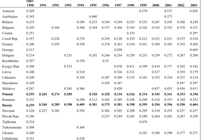
Table 1, based on most widely used published data, suggests that all the countries in Eastern Europe and the former Soviet Union experienced an increase in inequality. However, despite an apparently common legacy, countries witnessed very different degrees of increased inequality. On the one hand, as already seen in the example of Russia, a rapid increase in inequality occurred in the middle-income and low-income CIS countries, followed by some moderation. On the other hand, as the example of Poland at least till the middle of the 1990s illustrates, the new member states of the European Union (the EU-8), appear to have experienced a more gradual but steady increase in inequality. Table 1 makes clear that, by the early 2000s, the region exhibited the full spectrum of inequality outcomes, ranging from fairly unequal to fairly equal distributions of income.
Table 1. Gini indices for per capita incomes from “official” sources
1987-1990 1991 1992 1993 1994 1995 1996 1997 1998 1999 2000 2001 2002 2003 Armenia 0.269 0.570 0.537 0.428 Azerbaijan 0.345 0.440 0.373 Belarus 0.233 0.280 0.253 0.244 0.249 0.253 0.235 0.247 0.245 0.246 0.249 Bulgaria 0.245 0.344 0.340 0.384 0.357 0.366 0.345 0.326 0.332 0.333 0.370 0.351 Croatia 0.251 0.333 0.29* Czech Rep 0.197 0.228 0.270 0.258 0.230 0.239 0.212 0.232 0.231 0.237 0.234 Estonia 0.240 0.395 0.350 0.370 0.361 0.354 0.361 0.389 0.385 0.393 0.402 Georgia 0.313 0.430 0.469 Hungary 0.214 0.231 0.242 0.246 0.254 0.250 0.253 0.259 0.272 0.267 0.268 Kazakhstan 0.297 0.330 0.35 Kyrgyz Rep. 0.308 0.353 0.470 0.411 0.399 0.414 0.377 0.382 0.342 Latvia 0.240 0.310 0.326 0.321 0.327 0.358 0.379 Lithuania 0.248 0.350 0.347 0.309 0.332 0.343 0.355 0.354 0.357 0.318 Macedonia 0.349 0.369 0.367 0.34* 0.34* Moldova 0.267 0.365 0.360 0.420 0.437 0.435 0.436 0.411 Poland 0.255 0.265 0.274 0.285 0.320 0.328 0.334 0.326 0.334 0.345 0.341 0.353 0.356 Romania 0.232 0.290 0.312 0.302 0.305 0.298 0.299 0.310 0.353 0.349 0.352 Russia 0.259 0.260 0.289 0.398 0.409 0.381 0.375 0.381 0.398 0.399 0.394 0.396 0.398 0.404 Slovenia 0.220 0.227 0.282 0.250 0.302 0.305 0.298 0.299 0.310 0.353 0.22* 0.22* Slovak Rep. 0.186 0.237 0.249 0.262 0.249 0.264 0.263 0.267 0.299 Tajikistan 0.334 0.470 Turkmenistan 0.308 0.360 Ukraine 0.240 0.282 0.288 0.290 0.277 0.271 Uzbekistan 0.351 0.330
Source: Data from UNICEF TRANSMONEE 2005 edition [www.unicef-icdc.org/research], except for selected countries and years form ECAPOV I, Milanovic (1997), Poverty Assessments for Aremnia, Georgia, Uzbekistan, Ukraine, Tajikistan, and Eurostat (2005). Note: For Russia 1992 and earlier years data refer to total incomes, for later years – only to Money incomes;* data are form Eurostat and rely on a OECD per equivalent equivalence scale.
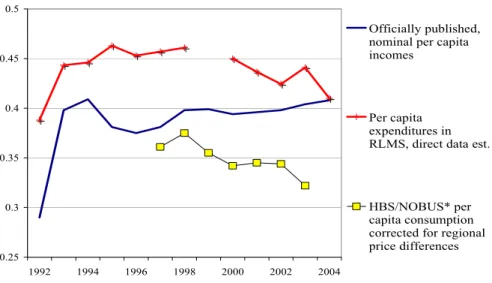
To what extent can the data presented in Table 1 be taken at face value? A flavor of the controversies surrounding the “stylized facts” depicted in the table is provided in Figure 3, which depicts a wide range of alternative inequality estimates for one country, Russia, drawn from different well-documented sources. The figure shows that, for the most recent period, Russia could be classified anything from a moderately high to a high inequality country or as anything from a country exhibiting rising to falling inequality, depending on the which source of data is chosen.
Figure 3. Russia: Evolution of Gini index from various sources, 1992-2004
0.25 0.3 0.35 0.4 0.45 0.5 1992 1994 1996 1998 2000 2002 2004 Officially published, nominal per capita incomes
Per capita expenditures in RLMS, direct data est.
HBS/NOBUS* per capita consumption corrected for regional price differences
Sources: Goskomstat, Poverty Assessment (World Bank ); RLMS- Russian Longitudinal Monitoring survey; HBS- Household Budget Survey; NOBUS – National Survey of Social Programs and Participation.
The example clearly illustrates the point that published data on income distribution should be treated with great care and this, following Atkinson and Micklewright (1992), for at least six different reasons:
First, published data from different countries rely on different imputation and adjustment procedures. In Ukraine, for example, significant and rather unusual imputations are undertaken with reported in-kind components. In some countries total incomes include imputed rents, whereas in others they do not: which option is chosen can have large effects. In Russia again, inclusion of owner occupied rents in 1993 reduced the Gini index from 0.42 to 0.35 (Buckley and Gurenko [1998]). Thus different rows in Table 1 cannot be compared with each other, and a higher country Gini does not necessarily translate into higher inequality for a comparable concept of welfare.
Second, in all the EU-8 countries, wages account for over 60 percent of household incomes. In contrast, among the low income countries of the CIS, wages represent less than 15 percent in some cases. At the same time, while public transfers are a much more important component of income in the EU-8, where they comprise 25 to 30 percent of total incomes; their importance has shrunk dramatically in the low income CIS countries to the point where
public transfers in Moldova and Georgia, for example, represent less than 10 percent of GDP.
Since wages and transfers can be measured quite well by household surveys, whereas other sources of income, such as from informal self-employment, are notoriously hard to measure with any precision, such compositional effects have serious implications for the accuracy with which inequality is measured. For this reason, Table 1 is a poor guide to describing inequality in the case of low income CIS countries such as Armenia, Georgia, the Kyrgyz Republic and Moldova.
Third, there are serious issues of under-reporting and non-response. Richer households, for example, tend to be increasingly missed by sample surveys. In practice, countries undertake different degrees of adjustment to correct for non-response but, in doing so, make a number of assumptions which can undermine comparability. In Russia, unlike in any other country, the increasing gap between reported incomes and estimates from macroeconomic sources is arbitrarily assigned to the top decile of households as “undeclared” incomes (World Bank 2005d), limiting comparability with other data on income distribution.
Fourth, correction for regional price differences is not normal practice in many statistical offices.1
Fifth, the use of equivalence scales has not been converging towards a single standard.2
All of this implies that, while official data can suggest that inequality has increased in all countries in transition, the magnitude of such increases is less certain. Despite these limitations, data such as those reported in Table 1 are used to generate “stylized facts” and draw far-reaching conclusions on the evolution of inequality in transition. [Ivashenko (2002)].
III. TOWARDS COMPARABLE DATA ON INEQUALITY IN TRANSITION
The lack of consistency of “official” data on inequality prompted the creation of comparable and consistent inequality statistics based on primary records from household surveys across the transition countries of Eastern Europe and the former Soviet Union.3 Most of these
surveys are conducted by statistical offices and are, in that sense, “official”. But the way in which primary data were used led to indices that are different from the numbers reported in Table 1.
First, the preferred measure of welfare is consumption rather than income. The choice of consumption was dictated by practical considerations. While data on incomes remain
1 When such corrections are practiced, they tend to reduce inequality as measured by Gini by between 1-3 percentage points.
2 The use of Eurostat equivalence scale rather than per capita with ECA household structure typically reduces the value of Gini index by about 2 percentage points.
3 Copies of much of the survey data conducted in the region are stored in the World Bank ECA regional data archive. At the time of writing the archive contained primary unit record data from recent household surveys for twentyfour countries spanning the period 1998-2004
particularly difficult to collect in transition countries, practice has shown that data on consumption can be gathered with considerable accuracy. Survey consumption modules have become more detailed over time and are better able to capture the various dimensions of consumption including, for example, informal payments.
Second, unlike the practice of simple aggregation undertaken by many statistical offices of the region, a distinction was made between different components of consumption. Since consumer durables and housing are consumed over a long period of time, it is customary to include the imputed value of the consumption flow associated with the possession of consumer durables (including housing) but to exclude the expenditure on the purchase of such goods. The lack of data, however, limits the application of this approach to all countries. It was therefore decided neither to include estimates of the flow of services of durables, nor durable purchases or rents.
Third, given the significance of spatial differences in the transition countries, an adjustment for spatial price differences was made, using Paasche price indices based on survey data in all countries. In cases where data were collected over a long period of time, it was also necessary to adjust for changes in prices over time. Quarterly CPI indices taken from IMF data were used to compute real values.
Fourth, households in the transition countries have coped with poverty by relying on an array of non-market strategies, including producing their own food and engaging in reciprocal exchange with other households and institutions. A consistent approach was used to assign a monetary value to these components of consumption.
Fifth, the same procedure, which conforms to methods used in other international household survey data depositories such as the Luxemburg Income Study, was used to clean the data of outliers across all data sets. Since a consistent approach was used across all data sets, one can be reasonably confident that differences across countries in the final consumption measure arise from differences in the primary data and are not owed to the method of aggregation.
Results for all countries with available primary records are presented in Table 2. The table clearly shows that there are discontinuities and that the evidence is of variable quality. However, the difference in country experiences regarding the evolution of inequality even with as comparable data as possible is striking. It dispels the notion that countries would converge to some common level of inequality that prevails in the long-run in market economies and provides motivation for the analysis undertaken in this paper. 4
4 Ravallion (2001), quoting Benabou (2000) argues that countries are expected to converge to the same distribution and proposes a test for such convergence, but due to data limitations transition economies have not been fully incorporated in his analysis.
Table 2. Gini index for comparable per capita consumption indicator Country 1988-1992 1993-1995 1996 1997 1998 1999 2000 2001 2002 2003 Albania 0.291 0.319 Armenia 0.444 0.321 0.325 0.310 0.285 Bosnia 0.263 0.295 Belarus 0.228 0.287 0.291 0.299 0.293 0.301 0.292 Bulgaria 0.234 0.283 0.350 0.337 0.277 Estonia 0.230 0.395 0.376 0.339 0.332 0.335 0.330 Georgia 0.28 0.370 0.404 0.386 0.393 0.397 0.383 0.390 0.391 Hungary 0.210 0.232 0.250 0.259 0.254 0.251 0.250 Kazakhstan 0.257 0.327 0.353 0.346 0.330 0.318 Kyrgyz Republic 0.260 0.537 0.523 0.405 0.360 0.346 0.299 0.290 0.292 0.276 Latvia 0.225 0.310 0.316 0.317 0.336 0.340 0.350 Lithuania 0.224 0.373 0.323 0.303 0.304 0.306 0.305 0.305 0.325 Macedonia 0.340 0.368 0.373 Moldova 0.241 0.343 0.371 0.365 0.350 0.357 0.345 0.328 Poland 0.235 0.264 0.268 0.277 0.296 0.302 0.305 0.307 0.320 Romania 0.255 0.282 0.274 0.283 0.282 0.286 0.294 0.289 Russia* 0.238 0.395 0.353 0.369 0.357 0.349 0.339 0.338 0.332 Serbia 0.292 Tajikistan 0.289 0.327 Ukraine 0.233 0.325 0.285 0.293 0.303 0.274 0.268 Uzbekistan 0.250 0.333 0.453 0.355 0.326 0.354
Sources: Figures in bold are from ECAPOV II, in italics – direct survey data estimates from other source
(ECAPOV I and PAs), other data are from WDI and Milanovic and are based on grouped data. Data for Poland in italic are from Keane and Prasad (consumption per capita without durables) and refer to 1990 for 1989-1992, Only figures from ECAPOV 2 are consistent across time. Notes: * based on HBS, except for 2003, where NOBUS data are used.
The new data confirm the overall picture that had emerged from the data on income inequality: Specifically, Table 2 shows that (1) all the transition countries have become more unequal; (2) there were rapid increases in inequality in many CIS countries, followed by some stabilization, or even subsequent moderation; (3) there was a much more gradual increase in Central Europe, with continued change up to the most recent year for which data are available; (4) there was a wide diversity of experience, even among countries within the same subgroup of countries. For example, the Baltic states experienced inequality paths similar to that of Russia, whereas the evolution of inequality in Belarus, which retains many features of a command economy, more closely resembled that in Central Europe. That said, the magnitude of increase and ranking of each country with respect to inequality usually differs, at times dramatically, from that provided by the income-based data in Table 1. Income-based and consumption-based measures of inequality appear to be fairly consistent with each other only in some cases, typically in the EU-8 countries. This is clearly not the case in the low income CIS countries and in some middle–income CIS and South Eastern European countries. For the reasons explained above, the new consumption-based data are
believed to be more accurate. Indeed it is consumption inequality, based on the new data, which is reported in Figure 1 on Poland and Russia used to introduce this paper.5
The data in Table 2 are also helpful in illustrating the evolution of inequality over time and decomposing its sources by household groups in countries that are deemed broadly representative of four clusters in the region, viz., Poland, Hungary and Latvia for the EU-8 countries, Romania for South Eastern Europe, Kazakhstan and Russia for the middle income CIS countries and Georgia, Moldova and Tajikistan for the low income CIS countries. Table 3 presents key data on the Gini index of inequality for those countries.
Table 3. Representative countries: inequality indices (Gini) for comparable per capita consumption Country Geor gi a Hun gar y Kaz akh st an La tv ia Mol do va Poland Rom ani a Russi a Ta jikista n Initial year/ End year 1999/2002 1993/2002 2001/ 2003 1998/2002 1998/ 2002 1998/ 2002 1998/ 2002 1997/ 2002 1999/ 2003 Gini index, initial year 0.397 0.232 0.346 0.336 0.371 0.296 0.274 0.353 0.289
Gini index, end year 0.391 0.250 0.318 0.350 0.328 0.320 0.289 0.338 0.327
Source: discussion in text
Having consistent data is the first step towards understanding the drivers for its increase and attempting to predict future evolution. The next section starts with two stylized “explanations” for the inequality increase often used to contrast various countries experience.
IV. MAIN DRIVERS OF INEQUALITY IN TRANSITION
To what extent can one appeal to the literature on inequality in transition for guidance on explanations of these disparate trajectories of growth and inequality? That literature suggests that the principal determinants of inequality in transition were:
• Wage decompression and growth of the private sector
• Restructuring and unemployment, reverting to subsistence economy
• Fiscal adjustment affecting Government expenditure and taxation, corruption • Price liberalization, inflation and arrears
• Asset transfer, growth of property income
• Technological change, increased mobility and globalization.
Driver 1. Wage decompression and growth of the private sector
Transition involved the emergence of a private sector which was to grow over time. By 2004, over 60 percent of GDP was produced in the private sector [EBRD (2005)]. This changed the process of wage setting by introducing a tighter link between productivity and wages. It is usual to associate inequality outcomes more closely to labor market conditions, primarily to inequality in wages, which in turn depends on the level of returns to human capital and changes in endowments. Indeed, wage inequality is a major driver of overall inequality. At a first glance, data on wage inequality data appear to mirror those for inequality of consumption. Contrasting different data sources, based both on enterprise records and household surveys, Figure 4 reports available Gini indices for wages in Russia and Poland. While dispersion between different sources is indeed very large, the levels and patterns resemble the trends depicted in Figure 1 closely.
Figure 4. Gini index for monthly wages in Russia and Poland, various sources
Russia Poland 0.2 0.25 0.3 0.35 0.4 0.45 0.5 0.55 1989 1991 1993 1995 1997 1999 2001 2003 Gi ni
Official wage, GKS RLMS ISSP
0.2 0.25 0.3 0.35 0.4 1989 1991 1993 1995 1997 1999 2001 Gi ni
Official, GUS HBS LFS ISSP
Sources: ISSP: International Social Survey Program from Paternostro and Tiongson Russia: Russian Statistical office (GKS), and RLMS – Russian Longitudinal Monitoring Survey, Lukianova for contractual wages (cleaning out the effect of arrears). Poland: HBS – Household Budget survey reported net wages Keene and Prasad, 2002 estimate –own; LFS –Labor Force Survey from Newell and Socha (2003).
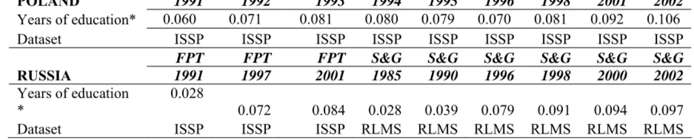
Why did wage inequality in Russia increase so rapidly? Returns to education alone seem to be insufficient to explain it. Cross country studies find that the returns to education increased from the “pre-transition” period to the “early transition” period. The meta-study by Fleisher and others (2004) suggests that the sharpest increases occurred during the early years of transition. Flabbi, Paternostro and Tiongson (2005) examine the evolution of the skills premium in transition economies through the late 1990s or the period thereafter through 2002 or 2003 using ISSP data, which is an internationally comparable survey. However, neither that study, nor the other sources reported in Table 4 below, produce any evidence that Russia stands out as having particularly large or distorted patterns of returns to education compared to Poland. Indeed it started with a much lower level of returns but already by mid 1990s had converged to Polish levels. This factor therefore cannot be used to explain excess inequality of Russian wages and other explanations are required.
Table 4. The Returns to Education in Russia and Poland
FPT FPT FPT FPT FPT FPT FPT FPT FPT
POLAND 1991 1992 1993 1994 1995 1996 1998 2001 2002
Years of education* 0.060 0.071 0.081 0.080 0.079 0.070 0.081 0.092 0.106
Dataset ISSP ISSP ISSP ISSP ISSP ISSP ISSP ISSP ISSP
FPT FPT FPT S&G S&G S&G S&G S&G S&G
RUSSIA 1991 1997 2001 1985 1990 1996 1998 2000 2002
Years of education
* 0.028 0.072 0.084 0.028 0.039 0.079 0.091 0.094 0.097
Dataset ISSP ISSP ISSP RLMS RLMS RLMS RLMS RLMS RLMS
Sources: Poland: FPT Flabbi et al. (2005); S& G) Sabrianova, K; Gorodnichenko, Y. “Returns to Education in Russia and Ukraine: A Semi-Parametric Approach…* Controls include: gender, location, age, family status.
Arrears as reported by Lehmann and Wadsworth (2001) were responsible for up to a third of
the “excess” inequality in wages in Russia. At the peak of wage arrears in November 1998, 64 percent of workers were owned back wages and the Gini index for wages actually paid was as high as 0.58. By 2004 the share of workers who were owed wages fell to 15 percent6
and the Gini index for paid wages fell to around 0.44, i.e. by just less than a third. But, even at this level, wage inequality was considerably higher than in Poland or other countries in Central and Eastern Europe. Therefore this factor, while providing a partial explanation for the inverse U-shape of the evolution of wage inequality in Russia, does not fully account for excess inequality in the distribution of earnings.
Another explanation is provided by distinct differences in minimum wages which were set at
around 40 percent of the average wage in Central and Eastern Europe, as opposed to at 10 percent of the average wage in Russia. [see World Bank (2005c)]. This allowed Russian firms to maintain low-paid jobs that otherwise would have been economically unviable, so that low minimum wages were a very important policy induced factor contributing to higher wage dispersion.
As opposed to relatively stable sectoral and inter-industry wage differentials, regional variation in real wages, relative to the national average, almost tripled in Russia between
1995 and 2003. Segmentation of labor markets is a common feature of many transition economies, but in Russia this dispersion takes particularly extreme forms due to institutional, infrastructure and geographical realities.
Increasing wage inequality in the transition countries of Eastern Europe and the former Soviet Union reflects a rising education premium, minimum wage policies and increased divergence of wages across sectors, regions and occupations. But wages, although important, were not the only determinant of inequality outcomes and the following factors played a role as well.
Driver 2: Restructuring and unemployment
Central to transition is the closure and restructuring of firms as resources are reallocated to more productive uses, together with the entry of new firms. Associated labor market developments have manifested themselves in a combination of (1) open unemployment, (2) lower labor force participation and (3) low productivity employment, such as subsistence agriculture or informal sector activities. A priori, there was little insight into what the incidence of job losses and its distribution across households would look like. Ex-post there are indeed important variations across countries and regions in the implied effects on inequality. The role of employment status as a contributor to inequality is examined in the decomposition of inequality among households partitioned by labor market status in Subsection V.2 below.
Driver 3. Changes in government expenditure and taxation
The system of social transfers was a sizeable factor initially thought to act to countervail increasing inequality. But in practice only in a few EU-8 countries, particularly Hungary, where social assistance programs expanded in real terms, did it have its intended effect. [Aghion and Commander (1998), Forster and Toth (1997), Garner and Terrell (1997), Keane and Prasad (2002a)]. In contrast, low-income CIS countries, faced with fiscal stringency, drastically reduced coverage of their safety nets to focus on the most needy. Other CIS countries aimed at retaining key benefits but compressed levels to a simple per capita distribution among the claimants. The role of transfers as a contributor to inequality is examined in the decomposition of inequality by source of income in Subsection V.1 below. On the revenue side, the transition induced a dramatic shift in the composition and incidence of taxes, such as the introduction of value added tax, while witnessing declining tax compliance. Limited empirical evidence suggests that most changes were in favor of greater equality, but with significant variation across countries and time periods [Kattuman and Redmont for Hungary, and Garner and Terrell for the Czech and Slovak Republics, and Commander and Lee who provide some evidence for Russia).
Driver 4. Price liberalization, inflation and arrears
All socialist economies embarked on the process of transition with a substantial monetary overhang [Flemming and Micklewright (1999)]. Hence, when prices were liberalized, they jumped and inflation rates tended to persist with accommodating monetary policy stance. Experience from other high inflation episodes (e.g. in Latin America) points to strong redistributive effects. And aggregate data indeed indicate that the inflation tax in Russia appears to have had a powerful effect. In 1992, for example, it has been estimated that households were hardest hit by inflation, losing about 12 percent of GDP through this tax on financial assets (Commander and Lee). This amounted to roughly a quarter of household income and is likely to have been regressive. Similar if not more redistribution took place in Georgia, Ukraine, Bulgaria, Belarus and Georgia, but did not substantially affect the EU-8 countries.
Arrears on pensions and social benefits payments appeared in the inflationary environment of several countries in the CIS and South Eastern Europe. Arrears were concentrated in the bottom part of the distribution and, in a highly inflationary environment, resulted in a cut in real wages in a highly unequalizing way (Lehmann and Wadsworth [2002]). Similar effects have been found by Klugman (2000) for Uzbekistan.
These factors were however largely transitory in nature and affected the shape of the distribution only in certain time periods.
Driver 5. Asset transfer and growth of property income
Perhaps the most visible sign of transition everywhere has been the large-scale transfer of previously publicly owned assets into the hands of private agents, a development that has produced a long-term shift in the distribution. The increase in the share of entrepreneurial income, and the share of families receiving financial incomes was an immediate result common to all transition economies. In Russia, for example, the share of property, interests and profits among households’ cash receipts increased from around 4 percent in 1989 to 20 percent in 2003 (Goskomstat). These sources of income are known to be unequalizing (Milanovic 1998). The role of entrepreneurial income as a contributor to inequality is examined in the decomposition by source of income in Subsection V.1 below.
Many privatization programs are believed therefore to have worsened the distribution of assets and income, at least in the short-run (Birdsall and Nellis [2003], Davies and Shorrocks 2005 for a review). As against this, it should be noted that a large part of national wealth was transferred in a rather equitable way through privatization of housing to tenants at below-market prices. In Russia, by early 1996 nearly 50 percent of the housing stock was in private hands, a proportion which had grown to 70 percent by 2005. Imputing an economic value to subsidized goods and assigning it to households in different parts of the distribution shows that this had mitigating effects on inequality (see Flemming and Mickewright 1999).
Driver 6. Technological change and globalization
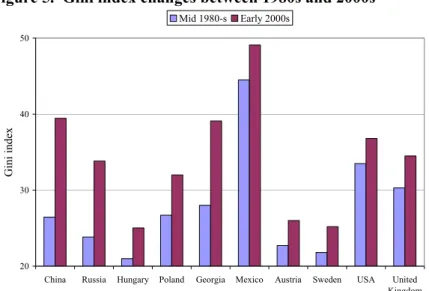
Technological change and modernization of the economy in a broad sense have been important in the evolution of inequality in many countries. Atkinson (2003) shows that transition economies were not alone in experiencing growing inequality: there has been an increase in inequality in many OECD countries on account of the change in technology associated with globalization, viz., a rise in the premium for skilled workers and a decline in the relative wage of unskilled workers. Figure 5 shows the extent of inequality increases in China, Russia, US, UK, Mexico, Sweden, Poland, Georgia and Hungary, using what is believed to be the most reliable indicator of dispersion in living standards for each country. The figure demonstrates that the increase in inequality in transition economies indeed occurred against the backdrop of a global increase in inequality with, however, important variations across countries. It is therefore inherently very difficult to separate transition-related determinants from the global factor of technological progress.
Figure 5. Gini index changes between 1980s and 2000s
20 30 40 50
China Russia Hungary Poland Georgia Mexico Austria Sweden USA United Kingdom Gi ni inde x Mid 1980-s Early 2000s
Source : ECAPOV2, Ravallion and Chen for China, LIS (www.lispoject.org) for other countries.
Note levels of Gini index are not comparable across countries as different concepts and definitions of welfare
are used. In ECA for 2002s: current consumption per capita without housing rental values, correcting for regional price differences and without outliers. Data for early 1980s come from published sources and refer to total expenditures, not correcting for price differences. China – total incomes per capita, correcting for price differences. OECD – per equivalent adult total money incomes, correcting for regional price differences without outliers.
How different drivers interact with each other is very much a question of particular country circumstances, initial conditions, and most importantly, policy choices. The taxonomy of drivers offers some basic insights into the reasons behind the variation across countries with respect to increases in inequality. Models of transition provide further guidance regarding the role of policies.
Models of restructuring
Aghion and Blanchard (1994) proposed a theoretical model of transition dynamics describing the reallocation of productive resources in transition. The transition is formalized as a reallocation of labor and capital across state and private sectors, with unemployment as a
transient step between the two7, and highlights ways in which endowments and policies in
transition affect the distribution of income (Commander and Tolstopiatenko [1996]).
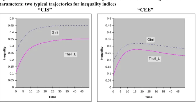
In the CIS, with an ungenerous benefits regime, and low initial values for closure and restructuring, the reallocation of labor to the private sector is protracted, and inequality rises gradually and steadily to high levels. More generous benefit regimes with higher probabilities of restructuring, as in Central Europe, lead to unemployment peaking at higher levels, but given a rapid movement of workers into the private sector and a generous floor in the form of unemployment benefits, the rise in inequality is less pronounced, reaching a hump at a lower level than that observed in the first scenario (Figure 6).
Figure 6. Simulation results from the restructuring model with different configuration of parameters: two typical trajectories for inequality indices
“CIS” “CEE” 0 0.05 0.1 0.15 0.2 0.25 0.3 0.35 0.4 0.45 0.5 0 5 10 15 20 25 30 35 40 45 Tim e In e q u a lit y Gini Theil_L 0 0.05 0.1 0.15 0.2 0.25 0.3 0.35 0.4 0.45 0.5 0 5 10 15 20 25 30 35 40 45 Tim e In e qua li ty Theil_L Gini
Source: Commander, Simon and Andrei Tolstopiatenko (1997).
An attractive feature of the model is the conceptualization of restructuring: not as one–time shift in the behavior of agents, but as a whole array of outcomes with different degree of rent appropriation by insiders in partly restructured enterprises. The empirical study of the first ten years of transition revealed the coexistence of new, partly restructured and unrestructured firms as a defining feature of the move from a command to a market economy (World Bank 2002e). This introduces an additional source of variability and hence inequality, which is captured by the model.
However, a comparison of predictions from the model with empirical evidence shows a surprising reversal of patterns between Central and Eastern Europe and the CIS. The inverse U-shaped trajectory of inequality seems to emerge not in the CEE, but in some CIS countries. The failure of the model to predict the actual evolution of inequality may be a result of its limitations of the model8, or alternatively the effect of mitigation of inequality through
offsetting policy measures.
Despite these limitations, the ability of the model to portray a large variation in the levels and shape of the development of inequality is instructive. It suggests that there is probably no single “transition” story as far as the evolution of inequality is concerned. Furthermore, the model results are broadly consistent with the story emerging from the earlier description of different drivers as being one which can yield a wide variety of outcomes across countries
8 This is essentially a model of labor reallocation which omits capital (or mixed) income, thereby by-passing one of the most important features of transition. Furthermore, parameters of the distribution within each sector are taken as exogenous and constant.
and over time. A number of these factors are directly or indirectly influenced by policies which have a role to play in the development of inequality.
V. DECOMPOSING INEQUALITY CHANGE IN TRANSITION
The most direct approach to capturing the relative importance of thee drivers empirically is to decompose inequality into its components and associate each component with a particular channel of redistribution. The structure of inequality by income source can be looked at in two ways: as inequality coming from between and within-economic group differences. Following A. Shorrocks (1982), the contribution of each component of income to total inequality can be obtained from the product of (i) the concentration coefficient for each component and (ii) the respective weights of those components in total income. Concentration coefficients in turn depend on how unequally an income source is distributed (“own Gini”) and how closely it is correlated with total incomes.9 The product of the share
of a particular type of income, and its concentration coefficient equals the contribution of that income component to the Gini index. The sum of these contributions equals the Gini index. Following Milanovic (1998), the main income sources taken to represent key drivers of the level and changes in inequality in this analysis are: wage income, pensions, social transfers and non-wage income (a combination of all other income sources, ranging from in-kind subsistence income, farm incomes, remittances to property income and incomes from self-employment and entrepreneurial activities). This stylized framework, by focusing on the relative importance of structural shifts versus own (or within-) inequality effects, is helpful in understanding how inequality levels changed during transition.
Given its potential for an analytical description of changes in the sources of inequality, it is somewhat surprising that there are only a few studies which use this framework (see Commander at al., Shutz, Kattuman and Redmont, Kyslitsyna). This section of the paper performs such decomposition exercises going back fifteen years, as opposed to the hypothetical exercises presented by Milanovic (1998), to understand the implications for inequality of employment reallocation between shrinking state and growing private sectors. Subsection V.1, which follows, looks at the evolution of the structure of income over time and the contribution of each component to inequality in Russia and Poland over the period 1987 through 2002, the choice of these countries being dictated by data limitations. Next, subsection V.2 presents group-based decompositions using data on consumption inequality for a larger group of countries. These are the key contributions of this paper.
V.1. Decomposition of inequality by income sources
Table 5 and Table 6 report levels and changes over time in the structure of incomes, the concentration coefficient of each component of income and its contribution to the Gini index of income inequality in Poland and Russia respectively.
9 Note that whenever the concentration coefficient of income source k is greater than the overall Gini coefficient, an increase in the income source k (holding everything else constant), will increase inequality.
The following points may be noted.
First, by the end of the period, the Gini index was seven points larger in Russia (0.41) than in Poland (0.34).
Second, the directions of change in the income structure in both countries were generally similar, reflecting transition-related drivers, viz., falling share of wages and a rising share of both entrepreneurial incomes (profits and income from self-employment) and pensions. The changes are consistent across periods of economic decline and growth, with wages and transfers moving in opposite direction. But the distributional outcomes were very different. Only to a limited extent were the differences due to changes in the composition of the source of income, such as the much steeper rise in social transfers (including pensions) in Poland compared to Russia. To examine to what extent these differences matter, it is not sufficient to simply compare actual changes across countries because the observed change is a complex result of interactions between drivers pulling inequality in different directions. What is needed is a counterfactual. However, producing a fully satisfactory counterfactual distribution is difficult and requires building a model of household income (Bourguignon et al), which goes beyond the scope of this paper. But it is feasible to conduct simulations using either base period concentration coefficients or income shares. It is recognized that such a counterfactual is purely hypothetical, because share and concentration often change for the same reason.
With this caveat in place, simple simulations show that the differences in the pace of structural change in income sources do not fully explain the inequality differential between Russia and Poland. In fact, an application of Poland’s income structure to Russia’s concentration coefficients yields a Gini index for Russia which is 0.5—1 point lower than it actually was. And application of Russia’s income structure to Poland would have led to a Gini index 2—4 points higher than actual in the latter country.
Table 5 Poland: Contribution of Income Sources to Total Inequality, 1987-2002
1987 1994 1998 2002 1994-1987 2002-1994 Income structure: percent
Work income 60 54 56 55 -6 +1
Of which wages 55 46 48 47 -9 +1
“entrepreneurial” 5 8 8 8 +3 +0
Income from farm 13 10 7 4 -3 -6
Old age pension 17 24 26 24 +7 +0
Social transfers 5 5 6 9 +0 +4
Other income 5 6 4 8 +1 +2
TOTAL 100% 100% 100% 100%
Inequality: Concentration Coefficients
Work income 0.260 0.330 0.388 0.431 +27% +31%
Of which wages 0.251 0.302 0.350 0.394 +20% +30% Entrepreneurial 0.360 0.488 0.613 0.650 +35% +33% Income from farm 0.415 0.390 0.471 0.575 -6% +47%
Old age pension 0.171 0.175 0.204 0.263 +3% +50%
Social transfers -0.100 0.080 -0.017 -0.011 +180% -86%
Other income 0.340 0.283 0.450 0.263 -17% -7%
Decomposition: Gini index, contributions
Gini, per capita inc. 0.250 0.280 0.320 0.343 +0.030 +0.063
Work income 0.156 0.178 0.217 0.237 +0.022 +0.059 Of which wages 0.138 0.139 0.168 0.185 +0.001 +0.046 Entrepreneurial 0.018 0.039 0.049 0.052 +0.021 +0.013 Income from farm 0.054 0.039 0.033 0.023 -0.015 -0.016 Old age pension 0.029 0.042 0.053 0.063 +0.013 +0.021 Social transfers -0.005 0.004 -0.001 -0.001 +0.009 -0.005 Other income 0.017 0.017 0.018 0.021 +0.000 +0.004
Source: Milanovic for 1987, ECAPOV I for 1994-1998 and Poverty assessment Staff calculations based on
CSO’s data for 2002.
The results are very different for the simulations focusing on the impact of changing concentration coefficients. Application of end-period concentration coefficients to Russia’s original income structure would have resulted in inequality exceeding its actually observed level by at least 5 percentage points. For Poland the result is striking: application of Polish end-period concentration coefficients to the original income structure would have resulted in a Gini coefficient of about 0.45, a level observed in Russia during this period and 10 points higher than the actual outcome in Poland (Figure 4).
This exercise shows therefore that changes in structure and in concentration coefficients offset each other, more so in Poland, but that the factors which increase inequality within income sources clearly dominate. Among these sources of change three need to be mentioned.
Table 6 Russia: Contribution of Income Sources to Total Inequality, 1989-2004
1989*** 1992 1996 1998 2004** 1998-1989 2004-1998 Income structure: percent
Work income 79 67 48 55 62 -24 +7
Wages 74 61 34 49 54 -25 +5
“entrepreneurial”* 5 6 14 6 8 +1 +2
Income from farm 4 8 15 11 8 +7 -3
Old age pension 8 10 18 20 17 +12 -3
Social transfers 7 6 2 2 2 -5 +0
Other income 2 9 17 13 11 +10 -1
Total income 100 100 100 100 100
Inequality: Concentration Coefficients
Work income 0.285 0.540 0.679 0.540 0.515 +90% -5% Wages 0.280 0.531 0.644 0.514 0.454 +84% -12% “entrepreneurial”* 0.360 0.633 0.764 0.750 0.925 +108% +23% Income from farm 0.300 0.350 0.440 0.573 0.375 +186% -35% Old age pension -0.200 -0.140 0.111 0.025 0.094 +113% +276% Social transfers 0.086 0.317 0.500 0.450 0.150 +425% -67% Other income 0.200 0.833 0.512 0.492 0.373 +146% -24%
Decomposition: Gini index, contributions Gini for income per
capita 0.22 0.47 0.51 0.45 0.41 +0.206 -0.024
Of which:
Work income 0.225 0.362 0.326 0.297 0.319 +0.072 +0.022 Wages 0.207 0.324 0.219 0.252 0.245 +0.045 -0.007 “entrepreneurial”* 0.018 0.038 0.107 0.045 0.074 +0.027 +0.029 Income from farm 0.008 0.028 0.066 0.063 0.030 +0.055 -0.033 Old age pension -0.016 -0.014 0.020 0.005 0.016 +0.021 +0.011 Social transfers 0.006 0.019 0.010 0.009 0.003 +0.003 -0.006 Other income 0.004 0.075 0.087 0.059 0.041 +0.055 -0.018 Method: decomposition of the Gini coefficient into components, ranking by total per capita income
Source: 1992-1998 from Commander et al based on RLMS, 2004 ** - own estimates based on RLMS data. ***1989-Milanovic based in HBS,* includes in-kind and cash incomes from non-agricultural self-emplyment,
informal work and property income.
First, labor income is the main source of livelihood, and distribution of earnings the main determinant of overall inequality. But the shape of the distribution is also determined by concentration. Increasing concentration coefficients of wages drove up the overall Gini coefficient in both countries, contributing around 25 points to inequality in Russia, and 18.5 points in Poland. The difference between these contributions, which is 6.5 Gini points, is almost the entire difference between the Gini indices for Poland (0.34) and Russia (0.41). At the same time, the concentration coefficient for wages in Poland (0.39 in 2002) is surprisingly large and not much lower than that for Russia (0.45 in 2004), despite the own Gini indices for wages, as shown in Figure 4, being significantly lower. This is due to different degrees of polarization of labor incomes in the two countries: in Poland a share of households as large as 47 percent (in 2002) did not receive any wage income compared to 35
percent in Russia (in 2004), reflecting inter alia a more sizeable adjustment in employment in Poland compared to Russia.
The second determinant of changes in inequality are transfers, pensions and other social benefits. The effect of transfers on inequality was not uniform, and changes were mostly driven by changes in the size and the distribution of pensions. In both countries changes in the distribution of pensions played a significant role as contributors to the increase in
inequality. But since their concentration coefficients were below those of market income sources, this expansion reduced inequality compared to potential levels. Had there be no
increase in transfers in Poland, inequality would have been fully 3 Gini points (or 10 percent) higher. The effects would indeed have been more progressive had there been no unequalizing change in the concentration coefficients of pensions.10 Other social transfers,
on the other hand, played a dramatically different role in Poland and Russia: thus, for example, the failure to target social benefits in Russia, as shown by a rapid increase in their concentration coefficient in early transition, is in sharp contrast to the situation in Poland. The third broad driver of inequality is private sector growth combined with increasing informality. The latter is difficult to measure with precision since the data cover reported incomes, which are known to underestimate informal incomes significantly [Yemtsov (1999)]. In particular it is important to distinguish between survival type activities, new entrepreneurial incomes and incomes from property. Informal income in various guises features in different parts of the income spectrum: (i) in farm income, in the form of in-kind consumption from own land plots, (ii) in entrepreneurial income, as many businesses are not registered or in the form of “side” wages reported as a result of “free-lancing”, or (iii) in “other income”, especially in the CIS where this term is often used as a euphemism for not fully legal or untaxed income. In terms of sheer size its effects were large. It is also quite remarkable that in the post-1998 crisis period in Russia some income sources with a strong informal component, such as farming and other incomes, show a fall in their concentration coefficients.
To summarize these results briefly, the comparison of Poland and Russia from the late 1980s to early 2000s finds that there is no single determinant of inequality; indeed, different drivers, at times working in opposite directions, combined to create a complex patchwork which is rich enough to allow a wide variety of outcomes. The analysis now turns to a more in-depth examination of spatial and other group-based factors of inequality.
10 This increase might seem somewhat counterintuitive, as transfers are often regarded as factors mitigating against inequality increase (Keane and Prasad [2002a]). Paradoxically, it was largely a result of the increased pensions and greater reliance on pension payments by recipients. Before transition inadequate pension payments were often supplemented by individual work post-pension age, and their recipients were as likely to be in the bottom of the distribution as in the top. After the changes in pension policy and indexation most pensioners moved to the middle of the distribution, while having to forego additional earnings with tighter labor markets. This created a stronger positive correlation between income level and pensions and hence larger concentration coefficients. Gustaffson and Nororozhkina (2005) used a unique study of households in Taganrog in 1989 and a follow-up study in 2000 to arrive at the same conclusions: the main beneficiaries from expanding public transfers have been households in the middle of the income distribution, and that also positively contributed to the increase of income inequality in Russia.
V.2. Decomposition of inequality by groups
A notable drawback of inequality decompositions based on components such as those presented in the previous subsection, is their reliance on income data, with the attendant problems of accurate reporting discussed in Section II of this paper.
However, with the population divided into groups affected by transition, total inequality can also be represented as the sum of inequality from within each of the groups and part of the
inequality coming from differences in means between these groups. Decompositions of
inequality by groups allow one to move to indicators of inequality in consumption, which is superior to income in terms of data quality.
This subsection decomposes consumption inequality in seven representative transition countries into the contribution of inequality ‘between’ groups and inequality ‘within’ groups using the Theil entropy measure of inequality (F. Bourguignon (1979) and A. Shorrocks (1980)). The sum of the within- and between-group contributions equals 1.
Table 7 A-C11 show to what extent inequality can be explained by inequality between
groups, such as (i) rural residents versus city dwellers, (ii) high school graduates versus those with less education, and (iii) working families versus jobless households. The choice of these partitions is designed to capture some key dimension of transition such as the emergence of new social classes and changing distribution within those classes. While none of them corresponds as neatly to a set of drivers of inequality as the distribution of income by source, they complement the story emerging from the decomposition of income in an important way. First, they identify winning and losing groups more clearly than is possible with decomposition by income source. Second, differences by educational attainment help assess the magnitude and dynamics of inequality effects related to technological change. Third, they add location effects, which account for a significant share of inequality in virtually every country, since transition resulted in changes in the concentration of economic activity and migration.
Urban-Rural (Location) (Table 7 A)
Changes in structure. There were significant changes in the distribution of population across
locations: in Hungary, the share of rural areas dropped from 38 percent to 35 percent of population during the period under review; in Latvia the share of Riga increased from 33 to 38 percent, and in Tajikistan the share of rural areas dropped from 78 to 73 percent in just 5 years. People have been migrating to higher income areas. As a result this driver reduced inequality. Had the initial distribution of population by location stayed the same, inequality in Latvia, for example, would have been 15 percent higher and that in Tajikistan 12 percent higher by 2003.
11 The Table relies on per capita equivalence scale, as Tables 3-4, where data availability dictated the choice. For Table 5 however, results are also available on per equivalent adult basis (with constant degree of returns to scale, θ0.5 or 0.75), results are broadly in line with reported (with exception of Moldova), and are available from authors on request.
Changes in “between” inequality. In general, consumption in rural areas is lower than in
urban areas. Capital cities have much higher living standards--in most cases about 40 percent higher consumption than the national average, even after controlling for price differences -- but also higher inequality. Over time, the relative position of rural areas has deteriorated in most countries, sometimes quite sharply. This indeed is common across all countries in Table 7A. As a result, the “between” component of consumption inequality went up everywhere except in Moldova, where it remained unchanged and in Hungary where it fell, the only case of clear convergence between locations.
Changes in “within”inequality. Within capital city inequality increased everywhere, again
with the exception of Hungary and stayed virtually the same in Russia. In rural areas, within-location inequality fell for the most part but remained broadly the same in Hungary and Moldova. There was no clear pattern for changes in inequality within other urban areas. Some part of the decline in inequality within rural areas may be linked to land ownership or use rights reforms. A broadly similar redistribution of land occurred in low income CIS countries such as Armenia and Moldova, which also have labor-intensive agriculture and where it is reasonable to expect the effects to have been equitable. Indeed, Table 7A also shows a large fall in the Theil entropy index in rural Moldova, as opposed to rural Tajikistan, where land reform has been much less comprehensive.
Regional factors
While the urban/rural dichotomy is small, the role of regional differences may be much greater. Thus, Yemtsov (2002), using official per capita income data series, shows that between-regional factors among Russia’s eighty-plus regions accounted for about a third of the overall inequality in that country by the year 2000, with the increase in the between-regions component being a key driver of the change in inequality between 1995 and 2000. However, direct survey measurements on consumption find the role of regional variation to have been much smaller: only about 15 percent of overall inequality can be ascribed to the between regional differences in means, with stability between 1997 and 2002 (World Bank 2005 d). Thus, while the persistence of regional factors is evident, their role as drivers of inequality change is not. Lack of convergence across Russian regions in mean real incomes is also presented as a major factor influencing the outlook for inequality going forward by Dolinskaya and by Fedorov.
Summing up, while locational factors play a role as a driver of inequality, it is unlikely that they will strongly influence the dynamics of inequality going forward. It is therefore necessary to focus on within-urban and, for low income CIS countries at any rate, within – rural drivers as key factors that will determine the evolution of inequality in the future.
Table 7. Decomposition' of Inequality: Share of between and within group inequality in Theil entropy index
A. By location (for inequality measured by consumption per capita)
Latvia Hungary Poland Romania Russia Moldova Tajikistan
1998 2002 1993 2002 1998 2002 1998 2002 1997 2002 1998 2002 1999 2002
Theil entropy measure 0.198 0.254 0.149 0.126 0.206 0.217 0.167 0.178 0.205 0.186 0.240 0.209 0.142 0.190 Decomposition of Theil inequality measure :
100% 100% 100% 100% 100% 100% 100% 100% 100% 100% 100% 100% 100% 100%
Of which between locations 6% 16% 5% 3% 5% 7% 3% 11% 3% 4% 9% 9% 3% 4%
of which within Capital city 37% 50% 30% 19% 5% 14% 8% 7% 22% 27% 9% 15%
of which within other urban areas 34% 19% 36% 49% 58% 51% 56% 58% 57% 70% 18% 14% 18% 20%
of which within rural areas 23% 16% 28% 29% 31% 28% 42% 31% 32% 19% 50% 51% 69% 62%
Theil entropy index for per capita consumption
Capital city 0.189 0.241 0.194 0.127 0.187 0.266 0.182 0.178 0.212 0.214 0.151 0.217
Other urban areas 0.189 0.177 0.124 0.124 0.198 0.195 0.157 0.160 0.177 0.181 0.230 0.176 0.158 0.213
Rural areas 0.184 0.189 0.125 0.116 0.189 0.190 0.170 0.154 0.258 0.168 0.218 0.184 0.131 0.169
Population shares
Capital city 33% 38% 19% 17% 4% 8% 6% 6% 17% 18% 6% 9%
Other urban areas 37% 32% 43% 48% 55% 52% 55% 54% 68% 68% 19% 19% 16% 18%
Rural areas 31% 30% 38% 35% 41% 40% 45% 46% 27% 26% 63% 63% 78% 73%
Real means, relative to national mean per capita consumption =1.00
Capital city 1.193 1.357 1.251 1.149 1.420 1.386 1.504 1.148 1.467 1.427 1.385 1.370
Other urban areas 0.976 0.852 0.993 1.024 1.093 1.088 1.085 1.181 0.980 1.065 0.998 0.882 1.032 0.999
B. By education of the household head (for inequality measured by consumption per capita)
Latvia Hungary Poland Romania Russia Moldova Tajikistan
1998 2002 1993 2002 1998 2002 1998 2002 1997 2002 1998 2002 1999 2002
Theil entropy measure 0.198 0.254 0.149 0.126 0.206 0.217 0.167 0.178 0.201 0.181 0.240 0.209 0.142 0.189 Decomposition:
Decomposition: 100% 100% 100% 100% 100% 100% 100% 100% 100% 100% 100% 100% 100% 100%
of which between education
group 7% 22% 11% 12% 13% 26% 11% 20% 2% 5% 8% 8% 4% 4%
Of which within primary
education 15% 9% 23% 19% 18% 14% 32% 25% 5% 2% 24% 21% 28% 22%
Of which within second education 54% 34% 5% 5% 26% 19% 25% 25% 31% 29% 32% 38% 24% 35%
Of which within vocational
education 4% 6% 38% 40% 24% 21% 19% 18% 39% 37% 23% 18% 27% 18%
Of which within tertiary
education 20% 28% 22% 23% 19% 20% 13% 13% 22% 27% 14% 15% 17% 21%
Theil entropy index for per capita consumption
Within primary education 0.158 0.171 0.136 0.105 0.165 0.181 0.155 0.145 0.256 0.159 0.219 0.166 0.126 0.202
Within secondary education 0.189 0.189 0.110 0.095 0.184 0.130 0.139 0.138 0.193 0.176 0.237 0.214 0.141 0.175
Within vocational education 0.267 0.195 0.113 0.109 0.163 0.158 0.139 0.139 0.207 0.177 0.220 0.189 0.136 0.176
Within tertiary education 0.183 0.224 0.188 0.125 0.208 0.195 0.169 0.153 0.176 0.164 0.203 0.189 0.148 0.178
Population shares
Primary education 23% 21% 30% 28% 24% 22% 40% 39% 5% 3% 31% 30% 34% 22%
Secondary education 58% 48% 7% 7% 27% 28% 28% 33% 40% 39% 35% 40% 26% 42%
Vocational education 4% 11% 52% 49% 38% 37% 25% 20% 34% 34% 23% 19% 27% 18%
Tertiary education 15% 19% 12% 17% 11% 13% 8% 8% 22% 24% 11% 11% 13% 18%
Real means, relative to national mean per capita consumption =1.00
Primary education 0.814 0.644 0.844 0.824 0.827 0.789 0.884 0.789 0.902 0.794 0.842 0.866 0.922 0.919
Secondary education 0.980 0.944 1.138 1.079 1.150 1.263 1.084 0.981 0.904 0.880 0.922 0.930 0.942 0.902
Vocational education 0.902 0.761 0.962 0.962 0.817 0.692 0.915 1.123 0.997 0.986 1.092 1.061 1.034 1.108
C. By household labor market status (for inequality measured by consumption per capita)
Hungary Poland Romania Russia Moldova Tajikistan Georgia
1993 2002 1998 2002 1998 2002 1997 1999 2002 1998 2002 1999 2002 1999 2002
Theil entropy measure 0.087 0.107 0.152 0.181 0.128 0.149 0.218 0.214 0.193 0.24 0.209 0.149 0.187 0.279 0.271
Decomposition
: 100% 100% 100% 100% 100% 100% 100% 100% 100% 100% 100% 100% 100% 100% 100%
of which between LM groups 2% 2% 1% 0% 4% 1% 0% 1% 5% 9% 8% 2% 0% 3% 1%
of which within LM group of wage
earners 52% 53% 38% 40% 55% 69% 62% 63% 67% 43% 38% 13% 40% 17% 19%
of which within LM group of
self-employed 16% 15% 43% 38% 18% 7% 5% 9% 14% 10% 18% 19% 39% 41% 39%
of which within LM group of
subsistence farmers 2% 2% 3% 3% 11% 8% 26% 19% 8% 29% 19% 66% 14% 29% 28%
of which within LM group of
non-working 27% 27% 15% 18% 13% 14% 6% 8% 6% 8% 16% 1% 6% 11% 13%
Theil entropy measure
within "formal" wage earners 0.084 0.104 0.145 0.171 0.118 0.142 0.194 0.207 0.184 0.239 0.208 0.171 0.21 0.228 0.205
within "informal" of self-employed 0.077 0.096 0.157 0.189 0.156 0.243 0.172 0.2 0.203 0.277 0.213 0.159 0.17 0.239 0.247
within "informal" subsistence farmers 0.086 0.089 0.146 0.202 0.121 0.133 0.339 0.233 0.156 0.187 0.134 0.138 0.16 0.339 0.354
within LM group of non-working 0.092 0.114 0.147 0.180 0.126 0.149 0.196 0.221 0.18 0.196 0.243 0.433 0.24 0.368 0.325
Population shares
"formal" wage earners 66% 56% 41% 43% 61% 56% 68% 62% 67% 36% 32% 11% 35% 20% 23%
"informal" self-employed 8% 15% 43% 37% 14% 18% 7% 9% 12% 7% 16% 15% 42% 50% 45%
"informal" subsistence farmers 1% 3% 2% 2% 13% 13% 17% 20% 14% 48% 38% 74% 17% 20% 20%
LM group of non-working 26% 27% 15% 17% 12% 13% 7% 8% 8% 9% 13% 0% 5% 10% 12%
Real means, relative to national mean per capita consumption =1.00
"formal" wage earners 1.022 0.97 0.988 0.992 1.059 1.077 1.02 1.042 1.055 1.222 1.193 1.071 1.011 1.046 1.086
"informal" self-employed 1.089 1.172 0.967 0.988 0.824 0.816 0.929 1.037 1.116 1.152 1.095 1.17 1.018 0.942 0.941
"informal" subsistence farmers 0.845 1.041 1.249 1.263 0.911 0.899 0.99 0.865 0.693 0.784 0.774 0.956 0.955 1.212 1.081
LM group of non-working 0.921 0.968 1.092 1.01 1.006 1.023 0.903 0.963 0.891 1.161 1.071 1.05 0.931 0.785 0.916