NBER WORKING PAPER SERIES
DEFLATION: PREVENTION AND CURE Willem H. Buiter
Working Paper9623
http://www.nber.org/papers/w9623
NATIONAL BUREAU OF ECONOMIC RESEARCH 1050 Massachusetts Avenue
Cambridge, MA 02138 April 2003
This paper is an extended version of the 2003 JSG Wilson Lecture in Economics, given at the University of Hull, 5th February 2003, under the title “The return of deflation: What can central banks do?” I would like to thank Anne Sibert for helpful comments and Toshiaki Sakatsume for able research assistance. The views and opinions expressed are those of the author. They do not necessarily represent the views and opinions of the European Bank for Reconstruction and Development or the National Bureau of Economic Research. ©2003 by Willem H Buiter. All rights reserved. Short sections of text not to exceed two paragraphs, may be quoted without explicit permission provided that full credit including ©notice, is given to the source.
Deflation: Prevention and Cure Willem H. Buiter
NBER Working Paper No. 9623 April 2003
JEL No. E31, E62, E63, F41
ABSTRACT
After an absence of almost half a century, the spectre of deflation is once again haunting the corridors of central banks and finance ministries in the industrial world. While preventing or combating deflation poses some unique difficulties not present in preventing or combating inflation, deflation can be prevented and, if it has taken hold, can be overcome, using conventional instruments of monetary and fiscal policy. These include open market purchases of government securities and monetary financing of government deficits caused by expansionary fiscal measures. Base money-financed tax cuts or transfer payments
n
the mundane version of Friedman’s helicopter drop of moneyn
will always boost aggregate demand.Unconventional monetary and fiscal measures are also available. These include open market purchases of private and foreign securities, negative nominal interest rates (through a carry tax on currency) and temporary tax measures aimed at shifting private consumption from the future to the present, by tilting the intertemporal terms of trade. An example is a cut in VAT today coupled to the credible commitment of a VAT increase in the future.
Deflation results from a combination of bad luck and poor economic management, including the failure to coordinate monetary and fiscal policy. Sustained unwanted deflation is evidence of policy failure. Both the knowledge and the tools exist to prevent unwanted deflation.
Willem H. Buiter
Chief Economist and Special Counselor to the President European Bank for Reconstruction and Development One Exchange Square
London EC2A 2JN UK
and NBER
Introduction
After an absence of almost half a century, the spectre of deflation is once again haunting the corridors of central banks and finance ministries in the industrial world.
The great deflations of the 19th century and 1930’s made way for the post-World War
II era of persistent inflation - low to moderate in the advanced industrial countries, moderate to high with occasional bursts of hyperinflation in developing countries, transition countries and emerging markets. The recent renewed concern with deflation is due in part to the historical association, at least during the interwar years, of deflationary episodes with financial crises, recession, stagnation and even depression. It is also prompted by the fear that in deflationary conditions, nominal interest rates may come close to their lower bound of zero, at which point monetary policy is thought to lose most if not all of its effectiveness.
I define deflation to be a sustained decline in the general price level of current goods and services, that is, a persistently negative rate of inflation. In principle, the price index is the ideal cost of living index. Real-world approximations include the Consumer Price Index (CPI) in the US, the Retail Price Indexes (RPI, RPIX and RPIY) in the UK and the Harmonised Index of Consumer Prices (HICP) in the EMU area. For many practical and policy issues, the distinctions between these indices are
important. For the purpose of this paper, they are irrelevant.1
1 There is a widely held view that real-world price indices present us with systematically upward-biased estimates of true inflation. This is important for issues ranging from cost-of-living indexation to the choice of an appropriate inflation target by the monetary authority. For reasons of space I will not consider these issues here. A Commission headed by Michael Boskin studied the CPI bias and presented the results of its report on December 5, 1996. It concluded that that CPI inflation in the US was likely to overestimate true inflation by about 1.0 percent to 2.0 percent per year. The sources of this bias in CPI inflation identified by the Boskin Commission were: 1. Substitution bias (0.2 - 0.4 points per year); 2. Outlet bias (0.1 - 0.3 points); 3. Quality changes (0.2 - 0.6 points); 4. New products (0.2 - 0.7 points); 5. Formula bias (0.3 - 0.4 points) (see Boskin et. al. [1996, 1997]). While not every aspect of the methodology used by the Commission, or the magnitude of the bias it found, have been universally accepted, there is widespread agreement that there was a significant upward bias. Changes made since then by the Bureau of Labour Statistics have probably reduced the magnitude of the bias.
What is important is that deflation as used in this paper refers to a declining
general price level for current goods and services. It does not refer to asset price
deflation – a fall in the prices of existing stores of value, either real or financial. Asset price movements are an important part of the transmission mechanism of monetary and fiscal policy actions and other shocks. Asset price movements often complicate the task of the monetary and fiscal authorities and prevent the simultaneous achievement of price stability, full employment and balanced structure of production and demand. Asset price deflation may at times precede, be associated with or even cause downward movement in the general price level of goods and services. Asset price deflation is, however, conceptually quite distinct from deflation in the sense used in this paper.
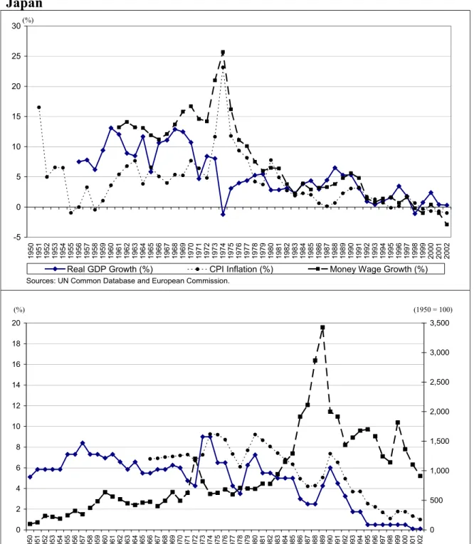
The timing of the renewal of political concern with and scholarly interest in deflation is not surprising. As shown in Figure 1, in Japan, the central bank discount rate has been at 50bps or less since 1995, raising concern about the zero lower bound on nominal interest rates, at least at the short end of the maturity spectrum. Japan is in a protracted economic slump that started in 1992. Money wages have declined in four of the past five years; the GDP deflator has declined in each of the past 5 years and the CPI in four out of the past 5 years. Short nominal interest rates in Japan are near
zero.2
Figure 1 here
2
Percentage annual growth rates of nominal price and wage indices in Japan
1998 1999 2000 2001 2002* Nominal Compensation** -0.7 -1.2 0.5 -0.1 -1.2 GDP Deflator -0.1 -1.4 -2.1 -1.2 -1.0 CPI 0.7 -0.3 -0.7 -0.7 -1.1
A number of observers have concluded that there is a liquidity trap at work, that is, monetary policy is incapable of stimulating aggregate demand (see e.g. Krugman [1998a, b, c, d; 1999, 2000], Ito [1998], McKinnon and Ohno [1999], Itoh, Motoshige and Naoki Shimoi [2000], Miyal [2000], Iwata, Shigeru and Wu [2001], Svensson [2001] and Taylor [2001]); for a view that liquidity traps are unlikely to pose a problem, see Meltzer [1999, 2001] and Hondroyiannis, Swamy and Tavlas [2000]).
The risk of the zero lower bound becoming a binding constraint on monetary policy has more recently become a factor also in Western Europe and the United States of America. In the Euro area inflation, on the HIPC measure, averaged 1.1 percent per annum during 1999. The ECB’s repo rate reached a local trough of 2.5 percent during April 1999. At the time, this raised the question as to whether a margin of two hundred and fifty basis points provided enough insurance against a slump in aggregate demand. In March 2003 the ECB’s repo rate again stands at 2.50 percent and HICP inflation runs at just over 2.0 percent per annum (Issing [2002]).
Figure 2 here
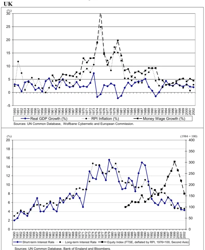
The UK has its Repo rate at 3.75 percent with RPIX inflation just over 2.5
percent.3 While this appears to provide a reasonable cushion against the risk of
getting stuck at the zero lower bound, the fear of deflation is not completely absent even in the UK.
Figure 3 here
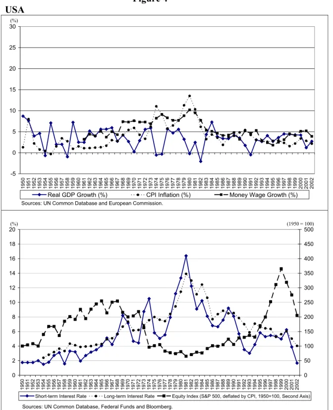
Finally, in the US too, with the Federal Funds target rate in February 2003 down at 1.25 per cent, the Fed has shown some concern about the possibility that monetary policy could become constrained by the zero lower bound on nominal
interest rates (see e.g. Bernanke [2002]). As early as the Fall of 1999, the Fed organised a conference to discuss the ‘zero bound problem’ (see e.g. Clouse, Henderson, Orphanides, Small and Tinsley [1999]) and recently its staff have produced a thorough study of Japan’s experience in the 1990s and the lessons this
holds for preventing deflation (Ahearne et. al. [2002]).4
Figure 4 here
There is also a growing number of theoretical contributions on liquidity traps, the zero bound problem, low inflation and deflation (see e.g. Akerlof, Dickens and Perry [1996], Fuhrer and Madigan [1997], Orphanides and Wieland [1998, 2000], Wolman [1998], Porter [1999], Johnson, Small and Tryon [1999], Cristiano [2000], Freedman [2000], Goodfriend [2000], Bryant [2000], McCallum [2000, 2002], Benhabib, Schmitt-Grohé and Uribe [2001, 2002], Buiter and Panigirtzoglou [2001, 2003], Feldstein [2002a,b] and Nishizaki and Watanabe [2002]).
The longest deflationary episode for which we have acceptable quality data is also the one that is probably most relevant for today. It is the great deflation of the
19th century, shown, for the UK, in Figures 5 and 6 .
Figure 5 here
Figure 6 here
As Figure 5 shows, the average rate of inflation over this 115-year period was slightly negative (certainly if we start our count at the end of the Napoleonic wars), and the variability of the inflation rate was high. Figure 6 shows that Bank Rate did
3 UK HICP inflation rates are between 0.50 percent and 0.75 percent per annum below its RPIX inflation rate.
4
not fall below 2 per cent throughout 115 years preceding World-War I.5 The UK got through a deflationary century without encountering the zero lower bound constraint on nominal interest rates, let alone the liquidity trap. The deflationary periods between the two World Wars are less relevant to our current experience. Although the failure to deal effectively with deflation no doubt prolonged and deepened the Great Depression of the 1930s, deflation then was the result of a catastrophic collapse of aggregate demand, not the cause of it.
Figures 5 and 6 demonstrate that deflation is an old phenomenon. Is it also an old problem? Deflationary episodes have often, but not always, been periods of recession or depression. Can policy makers prevent deflation or eliminate deflation once it has taken hold simply by reversing the policies that have been proven to be effective in preventing or eliminating inflation?
Some of the costs and benefits of deflation are not qualitatively different from the costs and benefits of inflation – there is no obvious discontinuity at zero inflation. For instance, menu costs (costs of changing prices) apply symmetrically to price
increases and to price cuts.6 Anticipated inflation causes welfare losses due to
shoe-leather costs of cash management if the opportunity cost of holding cash (the risk-free short nominal interest rate) increases with the expected rate of inflation. Deflation reduces the opportunity cost of holding non-interest bearing cash. Bailey [1956] and Friedman’s [1969] optimal quantity of money theorem is the proposition that welfare is maximised when the opportunity cost of holding money is zero, that is, when the risk-free nominal interest rate is zero. If welfare is maximised when the expected rate of inflation equals minus the short real interest rate, and if the short real interest rate is
5
The temporary collapse in the external value of the U.S. dollar starting in 1861 reflects the exceptional circumstances of the American Civil War and its aftermath, the Greenback period.
positive, deflation characterises the optimal monetary rule. In a Bailey--Friedman world, deflation is not a problem, it is part of the solution.
Unanticipated inflation redistributes wealth from creditors whose contracts are nominally denominated and not index-linked to debtors. Unanticipated deflation redistributes wealth from debtors to creditors. If and to the extent that higher inflation is associated with greater uncertainty about relative prices, higher inflation increases the noise-to-signal ratio of the price signals sent and received by households and enterprises. The same may well apply if the rate of deflation increases in absolute value.
There are four reasons why deflation is not just inflation with the sign
reversed. First, there is the problem of a zero lower bound on risk-free nominal
interest rates caused by the existence of stores of value with a risk-free zero nominal interest rate. These are coin and currency and commercial bank reserves with the
central bank.7 The zero nominal interest rate on base money (high-powered money,
the monetary liabilities of the central bank) sets a zero floor under risk-free nominal interest rates for all other stores of value, private and public. If in order to stimulate demand lower real interest rates are required but nominal interest rates are already at their zero lower bound, conventional monetary policy is powerless. Nominal interest rates are more apt to hit the zero floor when there is deflation.
Second, redistributions from debtors to creditors associated with unexpectedly high deflation in a world with imperfectly index-linked debt contracts is more likely to lead to default and bankruptcy than redistributions from creditors to debtors associated with unexpectedly high inflation. Default, bankruptcy and corporate
6 Menu costs do not, of course, attach only to changes in the prices of goods and services included in the CPI or GDP deflator. They presumably apply also to changes in money wages and intermediate goods and services and even to changes in the prices of existing assets.
restructuring are not just mechanisms for redistributing ownership and control of assets. These processes also destroy real resources.
‘Debt deflation’, the increase in the real value of nominal debt caused by a
falling general price level was considered an important source of financial distress by
the great monetary economists of the 19th century and the first half of the 20th century.
Irving Fisher [1932, 1933a] went as far as arguing that the interaction of deflation and large accumulations of private nominal debt could account for every major recession in the USA. Borrowers with short-maturity nominal liabilities and illiquid and/or real or foreign currency-denominated assets are especially vulnerable to deflationary shocks. Commercial banks fit that description, and the incidence of banking crises and bank defaults during the Great Depression of the 1930s and other severe recessions are consistent with a role for debt deflation in the propagation of the business cycle (see e.g. Fisher [1932, 1933a], Keynes [1931, 1936] and Haberler [1937]). Homeowners with mortgages or households with significant outstanding unsecured consumer debt have similar vulnerabilities in their portfolios, as do highly indebted enterprises, (see Minsky [1975, 1986] and King [1994]).
Hyman Minsky’s theory of financial fragility, distress and instability (Minsky [1975, 1986]) and modern theories of asymmetric information, adverse selection, moral hazard and agency problems in financial markets (see e.g. Bernanke [1983], Bernanke and Gertler [1995] and King [1994]) have sharpened our understanding of the links between balance sheet revaluations, access to credit and other sources of external finance, investment and consumption demand and fluctuations in output and employment.
7 There are countries where commercial bank reserves with the central bank are remunerated,
Third, there is a widely-held view that there exists an asymmetry in nominal wage and price adjustment. According to this view, the degree of downward rigidity in some nominal prices, and especially in money wages, is not matched by a similar
degree of upward nominal rigidity.8 This means that disinflation, the process of
bringing down the rate of inflation through a reduction in the growth rate of nominal demand will be more costly, in terms of output and employment foregone (that is, the
sacrifice ratio will be higher) when the inflation rate falls into the negative range than when it remains in the positive range.
Fourth, in living memory, there has been considerable experience of inflation, and even of hyperinflation, while there has been only limited experience of deflation (and none of hyperdeflation). This fourth point will turn out to be relevant also to the interpretation of the third point.
The proximate cause of deflation is the failure of nominal demand to grow at
least at the rate of growth of potential output. It may therefore be descriptively correct
that recent deflationary episodes have been the result of faster than expected productivity growth in some (significant) parts of the world – the USA and emerging Asia (China, India etc.) are often mentioned in this context. Even if, in an accounting sense, a reduction in inflation is associated mainly with an increase in real GDP growth driven by higher productivity growth rather than with a reduction in nominal GDP growth, such a diagnosis does not absolve the monetary and fiscal policy authorities. Whatever the supply-side of the economy may generate by way of a growth rate of potential output, it is always possible to use monetary and fiscal policy to generate any growth rate of nominal demand and therefore any rate of inflation, in
the medium term.9 Sustained deflation is therefore either a policy choice, or the result of policy failure.
1. Three Preliminary Questions
1.1 Why don’t we see negative nominal interest rates?
Financial instruments, henceforth securities, can be divided into two
categories: bearer securities and registered securities. Registered securities are financial instruments for which the identity of the owner is known to the issuer and can be verified by third parties. Bearer securities are financial instruments for which the owner is anonymous - the identity of the owner is unknown to the issuer and cannot be verified by third parties.
Paying interest, at a positive or a negative rate on registered securities is a simple task. Take, for instance, checking accounts or deposit accounts. The bank knows the owner of each account. Payment of interest at any rate, positive, zero or negative, is administratively straightforward. The bank periodically credits or debits
the account.10
With bearer securities, paying any non-zero interest rate is administratively non-trivial. If the interest rate is positive, care must be taken that the interest due is paid only once during a given payment period. Since the identity of the owner is unknown to the issuer, the same security could be presented multiple times during any
9 Former Governor Hayami [2002] of the Bank of Japan shows an appreciation of the relationship between technological change, changes in market structure, relative price changes and inflation in the following quote “At the same time, the basic relationships between structural reforms and prices must be correctly understood. The recent price decline is attributable to various factors such as
technological innovation, deregulation, and an increase in low-priced imports. But above all, the major factor is that Japan's economy was not able to achieve a full-scale recovery in the 1990s and that the negative output gap expanded due to lack of demand.”
10 Positive nominal interest rates on bank accounts have been common for decades. During the 1970s, the Swiss authorities taxed non-resident holders of Swiss bank accounts by paying a negative nominal interest rate during the 1970s. After allowing for bank fees, the net nominal rate of return on many checking accounts with a (low) positive nominal interest rate is frequently negative.
given payment period, either by the same holder or by a sequence of different holders. The way around this is to identify, label or mark the security rather than the owner. The security in question is marked in a verifiable manner by the issuer or his agent, whenever the security is presented for payment of interest due. Historically, bearer securities had coupons attached to them that were cut off (clipped) one at a time
whenever an interest payment was made.11 Other ways of identifying bearer
securities as being ‘ex-interest’12, such as stamping, or more high-tech identification
methods can no doubt be thought of.
If the interest rate on the bearer security is negative, the issuer faces the opposite problem of the holder not presenting himself to pay the issuer the negative interest due on the security. The solution is to find a way first of identifying the bearer security as being interest and second to ensure that securities that are not ex-interest are unattractive to potential owners.
The reason for the second condition becomes clear when one considers the bearer security that is of special interest for this paper: currency, that part of the monetary liabilities of the central bank that is generally accepted as means of payment
and medium of exchange in the central bank’s jurisdiction.13 14 Today, currency is
fiat money. It has no intrinsic value as a consumer good, a capital good or an intermediate input, other than the value of the paper it is printed on. It has value today if and only if the public believe it will have value tomorrow. For the issuer (the central bank) to put an expiry date on a bank note would be ineffective if the public chose to ignore it. To make paying negative interest on currency possible it must (a)
11 This would be problematic for a bearer perpetuity such as the British Consols.
12 I use ‘ex-interest’ analogously with ‘ex-dividend’ for common stock. A security is ex-interest for a given payment period if the interest due on it (positive or negative) has been paid.
13 And at times are accepted outside that jurisdiction, as with the US dollar and the Euro today. 14 The monetary liabilities of the central bank consist of currency in circulation and commercial bank balances with the central bank. Banks’ balances with the central bank are registered securities. The
be possible to identify bank notes as being ex-interest and (b) be possible to attach a
sufficiently severe penalty to holding money that is not ex-interest after the date the
interest is due. Fines, and, in the limit, confiscation or worse, would be required to enforce negative interest on currency.
The idea of taxing currency is not new. It goes back at least to Gesell and the
Social Credit movement in the second and third decades of the 20th century. No less
an economist than Irving Fisher viewed the idea sympathetically. (See Gesell [1949], Fisher [1933b], Porter [1999]). It has recently been revived and proposed by Buiter and Panigirtzoglou [2001, 2003] and by Goodfriend [2000]. Taxing currency by paying negative interest on it would be a costly administrative exercise. These costs must be set against the cost of being stuck at the zero nominal interest rate floor or the cost of pursuing a sufficiently high inflation target to minimise the risk of the zero nominal interest rate floor becoming a binding constraint.
1.2 Do asymmetric, downward nominal price and wage rigidities make deflation particularly costly?
Conventional economic theory has a rather easy time explaining real rigidities, but a hard time explaining any kind of nominal rigidities, let alone asymmetric nominal rigidities. Empirically there appear to be important nominal rigidities, but mainstream economic theory does a poor job explaining why the numéraire matters.
A fortiori, mainstream economic theory has little to say about asymmetries in the incidence and or severity of nominal rigidities. For instance, menu costs do not generate asymmetries between upward and downward price adjustments, although they can account for the spike in the frequency distribution of individual price
identity of the owner is known to the issuer. Any interest rate, positive or negative, can be charged on it with negligible administrative expense.
changes at zero. Neither do other state-contingent or time-contingent contracting
stories.15
Nominal price rigidity, symmetric or asymmetric, has never been attributed to nominal asset prices, or to the prices of freely traded homogeneous commodities. Its domain has never been argued to encompass more than the money prices of highly processed goods and services and to money wages. With nominal price cuts becoming more frequent in the low inflation environment of the last ten years (see e.g. the divergent behaviour of prices for goods and prices for services in the UK, shown in Table 1), those who argue for the importance of asymmetric downward nominal rigidity are focussing mainly on the labour markets (see e.g. Bewley [1999]).
Table 1 here
There is no coherent theory of asymmetric nominal rigidity in the labour market. Arguments based on fairness (Kahneman, Knetch and Thaler [1986], justice and morale miss the point, since fairness, justice and morale should concern real wages and/or relative real wages, over time and across reference groups, not money wages (see Blinder [1995], Akerlof, Dickens and Perry [1996], Card and Hyslop [1997] and OECD [2002]). Detailed micro-data based empirical studies for the UK, include Smith [2000] and Nickell and Quintini [2003] for the UK and McLaughlin [1994] for the US. The observation, painstakingly documented in hundreds of interviews by Bewley [1999], that both workers and managers will strongly resist money wage cuts can plausibly be attributed to the fact that the interviewees (in the 1990s) had known only positive inflation rates during their working lives. When nominal prices and wages have on average been rising for more than forty years, a
15 Surveys on price setting by supermarkets and other firms show a marked bunching of the frequency distribution of price changes at zero, for instance - but such observations tell us nothing about the existence of asymmetries in the degrees of downward and upward nominal price stickiness or rigidity.
nominal wage cut is likely to be a real wage cut also. Resisting a cut in money wages is a pretty good first stab at (indeed almost certainly a necessary condition for) resisting a real wage cut and, in decentralised labour markets, a relative wage cut.
Nickell and Quintini [2003], using a unique UK micro-date set on nominal wage changes for the period 1975-99, find that the proportion of individuals whose nominal wages fall from one year to the next is large (reaching 20 percent in periods of low inflation). They also find that there is evidence of some rigidity at a nominal wage change of zero. However, while this causes a statistically significant distortion in the distribution of real wage changes, the magnitude of the impact is “very
modest”.16
The policy relevance of even this very modest estimated impact is contingent on the degree of downward nominal wage rigidity being ‘structural’, that is, invariant under changes in the long-run rate of inflation. With high and even moderate inflation becoming a thing of the past throughout the industrial world, any nominal rigidities, and asymmetries in downward and upward nominal wage rigidity due to memories acquired and mental reference frames constructed during inflationary episodes will become less important as time passes. Finally, the spike in the empirical frequency distribution of contract wage changes at zero is, at most, evidence of nominal wage
rigidity, not of asymmetric nominal wage rigidity. I conclude that while there is
convincing empirical evidence that nominal price and wage rigidities exist, there is no evidence that these nominal rigidities are asymmetric.
1.3 How can we disentangle the effects of monetary and fiscal policy?
The distinction between monetary and fiscal policy instruments is an unimportant definitional issue. It sometimes gets tangled up with important issues involving the institutional arrangements for the decentralisation and delegation of the fiscal, financial and monetary management activities of the state. To understand the economic fundamentals that determine how monetary and fiscal policy affect aggregate demand, one should think of the central bank and the general government sector as a single, consolidated unit – the state, or the sovereign. The balance sheet, budget constraint and solvency constraint that matter are the balance sheet, budget constraint and solvency constraint of the consolidated general government and central bank. When we consider the practical, operational aspects of implementing certain policies in a specific country, it is indeed helpful to consider the particular institutional arrangements in that country. Often we will have to focus on the central bank as a separate agency of the state, with a distinct legal personality, charged with the management of the legal tender liabilities of the state and frequently also with the management of the official international foreign exchange reserves.
I could define monetary policy as ‘whatever the central bank does’, but a slightly more restrictive definition will turn out to be more useful in framing the analysis and organising the argument.
I consider four potential monetary instruments, one of them unconventional,
the other three conventional.17 The unconventional monetary instrument is the
nominal interest rate on base money (conventionally zero on coin and currency, but
16 They calculate that, if long-run inflation were to rise from 2.5 percent to 5.5 percent per annum, the equilibrium unemployment rate would fall from around 6 percent to around 5.87 percent (Nickell and Quintini [2003]).
17 I restrict the analysis to monetary and fiscal policy in reasonably well-functioning market economies. Quantitative credit controls and other government-imposed forms of credit rationing are not
not necessarily on the other component of the monetary base, commercial bank reserves held with the central bank). The three conventional monetary policy instruments are (1) the short risk-free nominal interest rate on non-monetary financial claims, henceforth the short nominal interest rate (in the UK this would be the 2-week Repo rate; in the US the Federal Funds rate, although the Fed does not peg that rate exactly); (2) the stock of base money; and (3), the nominal spot exchange rate (the relative price of foreign currency in terms of domestic currency). Of these four monetary instruments, the interest rate on base money will, except in Section 3.4c, be treated as a policy instrument whose value is set equal to zero. Out of the short nominal interest rate, the quantity of base money and the exchange rate, only one can be chosen independently by the authorities if there is unrestricted international capital
mobility and the country is small in global capital markets.18
In practice, countries either have a managed exchange rate (the exchange rate is the policy instrument) or they use the short nominal interest rate as the monetary instrument. I know of no country that uses (or used) the monetary base as the policy instrument, although in principle it is possible. Only when, in Section 4.3, I consider a rigorous version of Friedman’s ‘helicopter drop of money’, is the stock of base money treated as a policy instrument.
I define a conventional monetary policy action as any change in the quantity of base money, in the short nominal interest rate, or in the exchange rate which, at given prices and activity levels, does not change the financial net worth of the state (the consolidated general government and central bank), now or in the future.
considered. Changes in deposit reserve requirements are best viewed as fiscal measures (changes in the taxation of deposit-taking activities).
18 A ‘small’ country in a particular market is a price taker in that market. All countries except the US, can for practical policy purposes be treated as small in global capital markets.
Conventional monetary policy is therefore a subset of the state’s financial portfolio management. The state’s financial portfolio management comprises any changes in the composition of the government’s portfolio of financial assets and liabilities which, at given prices and activity levels do not change the financial net worth of the state now or in the future. This includes the sale and purchase of long-dated government debt instruments financed by matching changes in shorter-maturity instruments, changes in the currency composition of the government’s financial assets and liabilities (including sterilised and non-sterilised foreign exchange market intervention, changes in the mix of nominal and index-linked debt, public debt retirement financed through privatisation of state assets, swaps, trading in contingent claims markets etc).
Monetary policy involves a subset of such asset swaps. For our purposes, it always includes issuance or retirement (contraction) of base money financed through the purchase or sale of government interest-bearing debt (generally of a short maturity) or of foreign exchange reserves. Sterilised foreign exchange market intervention (purchases or sales of foreign in exchange for non-monetary liabilities of the government that do not alter the monetary base) also are generally conducted by the central bank. Note, however, that in the UK, most of the foreign exchange reserves are owned by the general government (the Treasury), although the Bank of England manages them as agent of the government. Most debt management operations not involving changes in the monetary base are no longer conducted by the Bank of England.
Fiscal policy includes any change in public spending or tax rules, regardless of whether they alter, at given prices and activity levels, the sequence of net financial balances of the state.
2. A Model of Aggregate Demand and Money Demand
The purpose of this Section is to present a simple formal model to guide the discussion of the conditions under which monetary and fiscal policy, conventional and unconventional, can or cannot stimulate aggregate demand. Monetary (and fiscal) policy ineffectiveness concerns the inability of monetary and fiscal policy to influence nominal aggregate demand. How a change in nominal aggregate demand is translated into changes in real GDP or in the general price level, depends on the details of the specification of the ‘supply side’ of the economy. As regards the key issues involved in preventing or curing deflation, the details of the determination of equilibrium prices quantities are irrelevant. Any combination of real output and general price level increases (including the two extremes of real output only and price level only) would be satisfactory. The paper therefore does not try to determine how any change in aggregate demand affects the general price level of prices of goods and services, real
output and employment, asset prices or other variable of interest.19 The detailed
derivation of the decision rules of Section 2 can be found in Buiter [2003].
There are two goods, domestic output and imports. Aggregate demand for
domestic output, e, is the sum of private consumption demand for domestic output,
H
c , private investment demand for domestic output, ιH, government spending on
domestic output, gH and export demand, x, that is,
H H H
e c= + +ι g +x (1)2021
19 In Buiter and Panigirtzoglou [2001, 2003], a simple continuous time, closed, endowment economy, represent agent version of the aggregate demand and money demand model developed here is combined with an old Keynesian (in Buiter and Panigirtzoglou [2001]) and a New Keynesian Phillips curve (in Buiter and Panigirtzoglou [2003]).
20 For brevity’s sake, we do not differentiate between public consumption spending and public sector investment.
21
, H, H, Hand
2.1 Households
There is a composite private consumption good that is a constant elasticity of substitution (CES) function of the consumption of domestic output and imports.
Consumption of imports is denoted cF, and aggregate consumption, measured in
terms of domestic output is
*
H F
SP
c c c
P
≡ + . The domestic currency price of domestic
output is P, the foreign currency price of imports is P* and S is the spot price of
foreign currency in terms of domestic currency, or the nominal spot exchange rate.
Let θ >0 be the static elasticity of substitution between private consumption of
domestic output and of imports, and let 0< ≤η 1. The CES price index for the private
domestic consumption bundle, P%, is given by
( )
(
)
( )
1 1 1 1 * 1 * (1 ) if 1 if =1 P P SP P P SP θ θ θ η η η η θ θ − − − − = + − ≠ = % % (2)Private consumption of domestic output is related to aggregate private consumption of the composite commodity as follows:
1 1 1 * (1 ) if 1 if 1 H P SP c c c P P c θ θ η η η η θ η θ − − − = = + − ≠ = = % (3)
The home country is fully specialised in the production of the domestic good. Domestic households supply the labour used in domestic production and own the
domestic capital stock. There are four stores of value, base money, M , issued by the
central bank, with a one-period nominal interest rate iM, one period nominal domestic
government bonds, B, with a one-period nominal interest rate i, one-period foreign
nominal value of a unit of installed capital is PK. All non-monetary stores of value are perfect substitutes in private portfolios and earn the same expected rate of return. Money yields direct utility (‘convenience services’) in addition to being a store of value.
Domestic output equals domestic value added in our model, which does not have imported intermediate or raw materials inputs. The proportional rate of change
in the price of domestic output, ( ) ( ) 1
( 1)
P t t
P t
π ≡ −
− is therefore also the GDP-deflator
rate of inflation. The real interest rate using domestic output as the numéraire, r, is
defined by 1 1 1 i r π + ≡ −
+ . Let Ω be the nominal value of the dividend paid out to
shareholders per unit of capital and let ξ be the proportional rate of depreciation of
the capital stock. Equalisation of expected rates of return on non-monetary assets then implies 1 1 [ ( 1) ( 1)] 1 ( 1) ( ) 1 K K t P t i t P t Ω + + +ξ + = + + (4) and * ( ) 1 ( ) 1 ( ) ( 1) S t i t i t S t + = + − (5)
There are two kinds of consumers. The first group always consumes its current disposable income. It neither saves nor borrows. This group is meant to capture the behaviour of consumers who are cash-flow constrained or liquidity-constrained; they have no liquid assets that they can draw down to finance consumption, nor can they obtain consumption loans. We refer to them as ‘Keynesian’ consumers. The aggregate real wage bill (measured in domestic output)
currently alive is assumed to earn the same wage and pay the same taxes. Aggregate
consumption by Keynesian consumers, cK is given by
( ) 0 1
K
c =λ w−τ ≤ ≤λ (6)
where λ is the fraction of the household population that is liquidity-constrained.
The second group of households has access to perfect financial markets. These ‘permanent income’ consumers can lend and borrow freely subject only to the constraint that the present value of their consumption programme not exceed the value of their initial net financial resources plus the present discounted value of their future after-tax labour income. Formally, we model these households using the discrete time version of the Yaari-Blanchard overlapping generations model (Yaari [1965], Blanchard [1985]) as generalised by Buiter [1988, 1990]. There is a constant birth
rate β ≥0, and a constant death rate, 1≥ ≥δ 0. There are perfect annuities markets,
so no-one leaves involuntary bequests. The individual’s probability of death is also the fraction of each age cohort (and therefore of the population as a whole) that dies in any given period. The probability of death raises both the effective subjective discount rate and the market rate of interest earned by surviving households. There is no other uncertainty. Agents have rational expectations. The aggregate consumption
of this group, cP, is proportional to its comprehensive wealth, the sum of its financial
wealth, aP, and its human wealth, hP
(
)
P P P
c =µ a +h (7)
In the model, all financial wealth, a, is owned by permanent income
consumers, so aP =a. The human wealth of a Keynesian consumer is the
same as that of a permanent income consumer; the difference between them is that the Keynesian consumer cannot borrow against the discounted value of
his future after-tax wage income. If economy-wide human wealth is denoted
h, it follows that hP = −(1 λ)h. Equation (7) can be rewritten as
[
(1 )]
P
c =µ a+ −λ h (8)
Economy-wide aggregate consumption is given by:
[ (1 ) ] ( )
P K
c c= +c =µ a+ −λ h +λ w−τ (9)
The law of motion for economy-wide financial wealth is given in equation (10).
[
]
( ) ( 1) [1 ( 1)] ( ) (1 )[ ( ) ( )] ( ) ( ) ( ) ( ) P M M t a t r t a t w t t c t i t i t P t λ τ + ≡ + + + − − − − − (10) and(
)
* *[
]
[1 ( )] ( ) ( ) [1 ( )] ( ) ( ) (1 ) ( ) ( ) ( ) ( ) ( ) K i t M t B t i t S t B t P t t K t a t P t ξ + + + + + − + Ω ≡ (11)Human wealth is the present discounted value of future after-tax labour income. Aggregate labour income is assumed not to be risky, so the appropriate discount rate is the risk-free real interest rate. Current consumption can only be driven by the human wealth owned by those currently alive. We calculate this by discounting future aggregate after-tax labour income at a higher rate than the risk-free
rate of interest. The difference is the birth rate, β, the rate at which ‘new entrants’
arrive to join the future labour force and the future cohorts of tax payers.
Note that the government will tax both current and future generations. The birth rate does not enter the government’s intertemporal budget constraint. If current generations were linked to future generations through an operative chain of intergenerational gifts and bequests, the birth rate will also be absent from the human wealth definition in equation (12) below.
[
1]
[
]
( ) ( ) ( ) 1 ( ) [1 ] j j t t h t w j j r β τ ∞ = = = − + + ∑
∏
l l (12)22The marginal propensity to consume out of comprehensive wealth, µ is given
in equation (13):
(
)
(
)
(
)
(
)
(
)
(
)
1 1 1 1 1 1 1 ( ) ( ) (1 ) [1 ( )](1 ) 1 ( ) 1 ( ) ( ) (1 ) 1 ( ) * 1 1 1 ( 1) ( 1) (1 ) j M t M j j t t M i j i j r t i i r i i ϕ σ ϕ ϕ ϕ σ ϕ α δ δ α α µ δ α α ρ δ α − = − ∞ − − = − = + − − + + + − = + − + + − + + − − − + ∏
∑
∏
l l l l l l l l 1 − (13)The expression for the marginal propensity to consume out of comprehensive wealth in (13) simplifies when future real and nominal interest rates are expected to be constant. In that case, we get
[
]
1 1 1 1 (1 )(1 ) (1 ) 1 ( )(1 ) (1 )(1 ) M r i i σ σ ϕ σ α δ ρ µ δ α δ ρ − − − − + + − + = + − + + + (14)When ϕ σ= =1 (logarithmic intertemporal preferences and a unitary elasticity
of substitution between the composite consumption good and real money balances), the marginal propensity to consume out of comprehensive wealth simplifies to the expression given in equation (15) below.
(1 )(1 ) 1 (1 )(1 ) 0; 0; 0 1 ρ δ µ α ρ δ ρ δ α + + − = + + > ≥ < ≤ (15)
Assuming that only permanent income consumers hold money balances, the demand for money is given by
22 We adopt the notational convention that ( ) 1
t
x =
[
]
(
)
( ) 1 1 ( ) [ ( ) ( )] ( ) ( ) ( ) (1 ) 0 1; 0; M M M t c t w t t P t i t i t i i ϕ α λ τ α δ α ϕ − = − − − + < ≤ > ≥ (16)The parameter ρ >0 is the subjective rate of time preference. The
intertemporal substitution elasticity is σ >0 and ϕ>0 is the static elasticity of
substitution between the composite consumption good and real money balances.
The demand for real base money depends negatively on the financial opportunity cost of holding money, that is, the excess of the short nominal interest rate over the short nominal interest on base money. The aspect of equation (16) that matters most is the second line, constraining the nominal interest rate on non-monetary financial claims to be at least as high as the nominal interest rate on base money. This floor on the nominal interest rate will be present as long as the non-pecuniary marginal utility of money does not become negative. A simple arbitrage
argument then suffices to establish the floor. Consider the case where iM =0. If the
short nominal interest rate on non-monetary assets could be negative, there would be risk-free way of making infinite profits by borrowing at the negative rate of interest and investing in base money. Our money demand function also has the property that the non-pecuniary marginal utility of money goes to zero only as the real stock of money balances relative to consumption goes to infinity, but that is not important for anything that follows.
2.2 The government
The government’s budget identity is given in equation (17) below and its intertemporal budget constraint or solvency constraint in equation (18). Note that government here means the consolidated general government and central bank.
Government non-monetary debt refers to general government debt held outside the
central bank.23 The government spends
H
g on domestic output, gF on foreign
output, raises taxes T in nominal terms, issues base money with a nominal interest
rate iM, issues domestic currency-denominated debt with a nominal interest rate i and
holds foreign exchange reserves D* that earn a nominal interest rate i*.24 We shall
call S t D t( ) *( )−B t( )−M t( ) the financial net worth of the government. Assuming
only households pay taxes to the government, we have T
P τ ≡ . We also define * H F SP g g g P ≡ + . * * * * ( 1) ( 1) ( ) ( 1) ( ) ( ) ( ) ( ) ( ) ( ) [1 ( )] ( ) [1 ( )] ( ) ( )[1 ( )] ( ) H F M M t B t S t D t P t g t S t P t g t T t i t M t i t B t S t i t D t + + + − + ≡ + − + + + + − + (17)
( )
* * [1 ( )] ( ) [1 ( )] ( ) ( ) ( ) 1 ( 1) ( ) ( ) ( ) 1 ( ) ( ) ( ) j M j t t i t B t i t S t D t P t M j M j j g j i j r τ P j P j ∞ = = + − + ∆ + = − + − + ∑
∏
l l (18)25We assume that government spending decisions can be represented by an exogenous sequence of aggregate public spending measured in domestic output,
{ ( );g j j t≥ }. International relative prices then distribute this aggregate across
domestic goods and imports according to equation (19) with 0< <ηˆ 1,θˆ>0 ,
1 ˆ ˆ 1 1 * ˆ ˆ ˆ ˆ (1 ˆ) 1 ˆ ˆ 1 H H H P SP g g g P P g θ θ η η η η θ η θ − − − = = + − ≠ = = (19)
23 In general, it would also include central bank non-monetary liabilities held outside the general government. We ignore this in what follows.
24 We assume for simplicity that the government earns the same interest rate on its international reserves as the private sector does on its foreign-currency-denominated securities.
Forward-looking permanent income consumers internalise the government’s intertemporal budget constraint. In equation (20) below, private aggregate consumption is represented after interest-bearing government debt is eliminated from the consumption function of the permanent income consumers given in (8), using (11) and the government’s intertemporal budget constraint (18). It aggregates the behaviour of the permanent income consumers who fully internalise the future taxes and monetary issuance decisions of the government, and the behaviour of the myopic Keynesian consumers.
(
)
[
]
* * * [1 ( )] ( ) [1 ( )] ( )[ ( ) ( )] (1 ) ( ) ( ) ( ) ( ) 1 1 (1 ) ( ) ( ) 1 ( ) (1 ) 1 ( ) ( ) ( ) 1 1 (1 ) 1 ( ) [1 ( )](1 ) K j j j t t t j j t t i t M t i t S t B t D t P t t K t P t w j g j r r c t t r r ξ λ β µ λ β ∞ = = = = = + + + + + − + Ω + − + + − + = + − − + + + ∑
∏
∏
∏
l l l l l l l l ( ) ( ) ( ) 1 ( 1) 1 ( ) ( ) ( ) [ ( ) ( )] j t j M j t t j i j M j M j r P j P j w t t τ λ τ ∞ = ∞ = = ∆ + + − + + −∑
∏
∑
∏
l l (20)The real value of a unit of capital carried into period t is (from equation (4))
given by the present discounted value of the future dividend stream:
( ) 1 ( ) ( ) (1 )[1 ( )] ( ) j K j t t P t j P t ξ r P j ∞ = = Ω ≡ + +
∑
∏
l l (21) 2.3 Private investmentThere is a composite private investment good, ι%, represented by a CES
function of domestic output and imports. The price index for the composite
investment good is, with 0< ≤η 1 and 0θ > ,
25 ∆ is the backward difference operator, that is, ∆M t( + =1) M t( + −1) M t( ).
( )
1 11 1 * * 1 (1 ) if 1 ( ) if 1 I P P SP P SP θ θ θ η η η η θ θ − − − − = + − ≠ = = % (22)There are quadratic internal adjustment costs associated with investment. Both the production function and the adjustment cost function are constant returns to
scale. Private investment can therefore be represented as a function of ‘Tobin’s q’.
With 0,v> we have, letting PI
P ι= % ι%: 1 1 1 * 1 * ( ) ( ) 1 ( ) ( ) ( ) ( ) 1 (1 ) ( ) ( ) 1 ( ) if 1 ( ) ( ) ( ) 1 ( ) ( ) 1 ( ) if 1 ( ) ( ) K I K K P t P t t K t v P t P t S t P t K t v P t P t P t S t P t K t v P t P t θ θ η ι η η θ θ − − − − = = + − − ≠ = − = % (23)
Private investment demand for domestic output is given by
1 1 * (1 ) if 1 if =1 H EP P θ ι η η η ι θ ηι θ − − = + − ≠ = (24)
Private investment demand for imports is denoted ιF.
2.4 Export demand
Without modelling the rest of the world in any detail, we want to specify
export demand for domestic output, x, analogously to the import demand functions
implicit in our specification of consumption, public spending and private investment. We therefore assume that the home country takes as given aggregate spending in the rest of the world in terms of foreign output, and that the ideal price index for foreign spending (the price, in terms of foreign currency) of some appropriate foreign
composite commodity, is * * * * * 1 1 1 * * *1 (1 *) P if 1 * and * * ( )P 1 if 1* P P P P S S θ θ θ η η η − η − − θ − θ = + − ≠ = = % % .
Let f* denote aggregate rest-of-the-world demand measured in foreign
output. Export demand for home country output is given by:
(
)
(
)
* 1 * * * * * * * * * * * 1 (1 ) if 1 1 if 1 P P x f SP SP SP f P θ η η η θ η θ − = − + − ≠ = − = (25)In the next Section, we study the effects of monetary and fiscal policy on aggregate demand using the model developed in this Section as a benchmark, but going beyond it where necessary.
3. Monetary Policy and Aggregate Demand
The model of aggregate demand for domestic output is summarised in equations (1), (3), (18), (19), (20), (21), (23), (24) and (25). In the formal model, the effect of conventional monetary policy on aggregate demand for domestic output
means the effect on current aggregate demand for domestic output, ( )e t , of changes in
the current short nominal interest rate, (i t+1),26 and/or credible announcements about
changes in one or more future short nominal interest rates, i j( ), j t> +1, holding
constant all other (expected) future short nominal interest rates. Also held constant
are the initial values of all asset stocks (money, M t( ), government debt, ( )B t , net
private holdings of foreign debt, B t*( ), foreign exchange reserves, D t*( ) and the
domestic general price level
{
P j( ), j t≥}
;27 (2) the nominal exchange rate{
S j( ), j t≥}
;(3) real wage income{
w j( ), j t≥}
; (4) real tax revenues{
τ( ),j j t≥}
; (5) aggregate real public spending{
g j( ), j t≥}
; (6) aggregate realspending in the rest of the world
{
f*( ),j j t≥}
; (7) nominal interest rates on basemoney
{
iM( ),j j t≥}
; (8) foreign nominal interest rates { ( ),i j* j t≥ }; (9) foreignprices { ( ),P j* j t≥ }; (10) capital rental rates
{
Ω( ),j j t≥}
; (11) seigniorage( 1),
M j j t
∆ + ≥ .
3.1 A cut in the current short nominal rate of interest
As long as the lower bound on the nominal interest rate is not binding ( (i t+ >1) i tM( +1)) the monetary authorities can reduce the current short nominal rate
of interest, i t( +1). A reduction in the current short nominal interest rate i t( +1)will
boost both private consumption demand and investment demand (because we allow
for endogenous changes in the value of capital, PK).
For n t≥
(
)
(
) (
) (
)
(
) (
)
( ) ( ) ( ) 1 ( ) 1 ( ) 1 ( ) 1 ( ) ( ) ( ) (1 ) ( ) 1 ( ) c t t a t h t i n i n i n t a t h t i n µ λ µ λ ∂ = ∂ + − ∂ ∂ + ∂ + ∂ + ∂ + + − ∂ + (26)In general, consumption demand is affected by changes in real interest rates
through three channels: the income effect, the substitution effect and the revaluation effect. In our model, the income and substitution effect work through the marginal
26 Note that i t( ) is predetermined in period t.
propensity to spend out of comprehensive wealth, µ. It is clear from equation (13) that the marginal propensity to spend out of comprehensive wealth will be independent of current and future real interest rates if and only if (1) income and substitution effects of a real interest rate change cancel each other exactly, that is, if
1
σ = and (2) the income effect and substitution effect of a change in i i− M, the
opportunity cost of holding base money, cancel each other out, that is, if ϕ=1. In our
model this will be the case if the period utility function is logarithmic in a Cobb-Douglas function of aggregate consumption and real money balances (see Buiter [2003]).
From equation (13), ceteris paribus, a lower real rate of interest (in the current
period or anticipated in the future) will raise (lower) the marginal propensity to
consume out of comprehensive wealth if and only if σ >1 (σ <1).28 Also, ceteris
paribus, a lower nominal rate of interest (in the current period or anticipated in the future) will raise (lower) the marginal propensity to consume out of comprehensive
wealth if and only if ϕ<1 (ϕ >1).29
This is intuitively obvious: if there is a sufficiently strong willingness to shift consumption between the present and the future in response to changes in intertemporal relative prices, a cut in current or anticipated future real interest rates will boost consumption. Also, if the elasticity of real money demand with respect to
28 For instance, from equation (14), the steady-state effect of a permanent change in the real interest rate on the marginal propensity to consume (holding constant the nominal interest rate) is
[
]
1 1 2 1 ( 1)(1 ) 1 ( )(1 ) (1 ) (1 )(1 ) M M M i i i i r i i r σ ϕ σ µ α σ δ α δ ρ − − − − = − ∂ − − + = − + − + ∂ + + + .29 For instance, from equation (14), the steady-state effect of a permanent change in the nominal interest rate, holding constant the real interest rate, is given by
the nominal interest rate is less than unity (in absolute value), a lower nominal interest rate will raise the share of consumption of the composite commodity in total spending on the composite commodity and the services provided by money balances.
In our Sidrauski-type model, money is not super-neutral unless both the intertemporal substitution elasticity and the elasticity of substitution between the
composite consumption good are equal to one.30 When only the elasticity of
substitution between money and consumption is unity, there will be no steady-state nominal interest rate effect on the marginal propensity to consume (equation (14)), but there will be temporary effects. Only when both the intertemporal elasticity of substitution and the elasticity of substitution between money and consumption are
unity (σ ϕ= =1, see equation (13)) will there be neither steady-state nor dynamic
effects of the nominal rate of interest on the marginal propensity to consume.
There is no consensus on the magnitude of the intertemporal substitution elasticity. Empirical studies based on the representative agent, time-separable expected utility paradigm in which the constant of relative risk aversion is the reciprocal of the intertemporal substitution elasticity, typically find that the intertemporal substitution elasticity is close to zero (or equivalently, that the degree of relative risk aversion is very high). Examples are Hansen and Singleton [1983], Hall [1988] and Yogo [2002]. Allowing the period felicity function to be non-separable in consumption and leisure can raise the (implied) estimate of the elasticity of
( )
[ ][
]
2 1 1 1 (1 )(1 ) (1 ) 1 ( )(1 ) (1 )(1 ) ( ) 1 ( 1) M ( )(1 ) (1 ) M r r M r i i i i i i σ σ ϕ σ ϕ α δ ρ δ α δ ρ µ α ϕ δ δ α − − − = − − + + + + − + + + ∂ = ∂ − − − − − + + intertemporal substitution to around 0.35 which, while significantly different from
zero is also significantly below one (see Basu and Kimball [2000]).
There have been four distinct approaches that attempt to rebut this finding. Mulligan [2002] argues that earlier studies measured rates of return incorrectly and that making the appropriate corrections yields results consistent with an intertemporal elasticity of substitution of one. The second rejects the representative agent assumption and models heterogeneous consumers/portfolio holders. For instance, Guvenen [2003], permits the intertemporal elasticity of substitution to increase with household wealth and assumes that many low wealth consumers do not participate in the financial markets at all (rather like the Keynesian consumers of this paper).
The third alternative drops time-separability, that is, the current period felicity function depends not just on current consumption, but also on past consumption. Habit formation is a portmanteau explanation for such specifications (e.g. Abel [2000]). Finally, the expected utility hypothesis has been dropped in favour of alternatives, such as the Epstein-Zinn [1989, 1991] utility functions, that allow intertemporal substation and risk aversion to be modelled and estimated independently (see e.g. Hyde and Sherif [2002]). An outsider trying to sum up the results of this literature can only conclude that it is difficult to argue that the intertemporal substitution elasticity is close to unity and virtually impossible to conclude that it is significantly above unity.
As regards the interest elasticity of the demand for base money, most
empirical studies do not favour the constant elasticity specification of the model.31
The popular log-linear specification implies a negative nominal interest rate elasticity whose absolute value starts at zero when the nominal interest rate is zero and
31 Few empirical studies use private consumption as the scale variable in the money demand function. Income (current or permanent) and financial wealth are more commonly found in that role.
increases without bound as the level of the nominal interest rate increases. When the nominal interest rate is near the zero floor, the (absolute value of the) interest elasticity of money demand is therefore likely to be less than one, which would strengthen the positive impact on aggregate demand of a cut in the nominal rate of interest.
The revaluation effect of a change in a real interest rate refers to the change in comprehensive wealth as some element in the sequence of current and future real interest rates changes (see equations (11), (12) and (20)). We can further distinguish the financial wealth revaluation effect and the human wealth revaluation effect.
The effect of a change in the period n real interest rate (n t≥ +1) on human
wealth in period t is:
[
]
[
]
[
]
[
]
( ) 1 ( ) 1 1 ( ) ( ) 1 ( ) 1 ( ) (1 ) j j n t h t r n w j j r n r β τ ∞ = = ∂ = ∂ + − − +∑
∏
l + l + (27)32The revaluation effect of a cut in the period n real interest rate (brought about
in our example by a cut in the period n nominal interest rate holding constant the
(anticipated) period n rate of inflation) is positive if after-tax labour income in period
n and beyond is ‘on average’ positive.
As regards the financial wealth revaluation effect, the lower real interest rate associated with a lower nominal interest rate at a given inflation rate will also boost
Tobin’s q, the market value of a unit of installed capital (see equation (21)).33 By
boosting q PK
P
≡ , both private consumption (equation (20)) and private investment
32 In equation (27), the government’s intertemporal budget constraint has not been substituted into the private sector comprehensive wealth definition.