3
Crisp-Set Qualitative
Comparative Analysis (csQCA)
Benoît Rihoux Gisèle De MeurAfter reading this chapter, you should be able to:
• Understand the key operations of Boolean algebra and use the correct conventions of that language
• Transform tabular data into Venn diagrams and vice versa; interpret Venn diagrams
• Replicate a standard csQCA procedure, step by step, using the software • In the course of this procedure, dichotomize your variables (conditions and outcome) in an informed way, and at a later stage, use an appropriate strategy for solving “contradictory configurations”
• Weigh the pros and cons of usinglogical remainders(non-observed cases) • Read and interpret the minimal formulas obtained at the end of the
csQCA
Goals of This Chapter
33
csQCA was the first QCA technique developed, in the late 1980s, by Charles Ragin and programmer Kriss Drass. Ragin’s research in the field of historical sociology led him to search for tools for the treatment of complex sets of binary data that did not exist in the mainstream statistics literature. He adapted for his own research, with the help of Drass, Boolean algorithms that had been developed in the 1950s by electrical engineers to simplify switching circuits, most notably Quine (1952) and McCluskey (1966). In these so-called minimization algorithms (see Box 3.2), he had found an instrument for identi-fying patterns of multiple conjunctural causation and a tool to “simplify com-plex data structures in a logical and holistic manner” (Ragin, 1987, p. viii).
csQCA is the most widely used QCA technique so far. In this chapter, a few basic operations of Boolean algebra will first be explicated, so the reader can grasp the nuts and bolts of csQCA. Then, using a few variables from the inter-war project (see Chapter 2), the successive steps, arbitrations, and “good prac-tices” of a standard application of csQCA will be presented.
T H E F O U N DAT I O N O F C R I S P - S E T Q C A : B O O L E A N A L G E B R A I N A N U T S H E L L
George Boole, a 19th-century British mathematician and logician, was the first to develop an algebra suitable for variables with only two possible values, such as propositions that are either true or false (Boole, 1847; 1958 [1854]). Following intuitions by Leibniz one century before him, Boole is the origina-tor of mathematical logic that allows us to “substitute for verbal reasoning a genuine symbolic calculation” (Diagne, 1989, p. 8). This algebra has been studied further by many mathematicians and logicians over the last few decades. It has been central to the development of electronic circuits, computer science, and computer engineering, which are based on a binary language, and has led to many applications, mostly in experimental and applied scientific disci-plines. Only a few basic principles and operations will be presented here (for more details, see, e.g., Caramani, 2008; De Meur & Rihoux, 2002; Ragin, 1987, pp. 89–123; Schneider & Wagemann, 2007, forthcoming). Boolean algebra, as any language, uses some conventions that need to be understood before engaging in csQCA.
It is a conception of causality according to which:
1. The mainconventionsof Boolean algebra are as follows:
• Anuppercaseletter represents the [1] value for a given binary variable. Thus [A] is read as: “variable A is large, present, high, . . .”
• Alowercaseletter represents the [0] value for a given binary variable. Thus [a] is read as: “variable A is small, absent, low, . . .”
• Adashsymbol [-] represents the “don’t care” value for a given binary variable, meaning it can be either present (1) or absent (0). This also could be a value we don’t know about (e.g., because it is irrelevant or the data is missing). It isnotan intermediate value between [1] and [0].
Box 3.1
With this very basic language, it is possible to construct very long and elab-orate expressions and also to conduct a complex set of operations. One key operation, which lies at the heart of csQCA, is calledBoolean minimization.
It is the “reduction” of a long, complex expression into a shorter, more parsi-monious expression. It can be summarized verbally as follows: “if two Boolean expressions differ in only one causal condition yet produce the same outcome, then the causal condition that distinguishes the two expressions can be con-sidered irrelevant and can be removed to create a simpler, combined expres-sion” (Ragin,1987, p. 93). Let us use a very simple example. Consider the following Boolean expression, with three condition variables (R, B, and I) and one outcome variable (O) (Formula1):
R * B * I + R * B * i O
This expression can be read as follows:“[The presence of R, combined with the presence of B and with thepresenceof I] OR [The presence of R, combined with the presence of B and with theabsenceof I] lead to the presence of out-come O.”
Notice that,no matter which value the [I] condition takes(0 or1), the [I] out-come value is the same. This means, in verbal reasoning, that the [I] condition is superfluous; it can thus be removed from the initial expression. Indeed, if we remove the [I] condition, we are left with a much shorter,reduced expression (which is called aprime implicant) (Formula 2):
R * BO
Box 3.2
What Is Boolean Minimization?
2. Boolean algebra uses a few basicoperators, the two chief ones being the following:
• Logical “AND,” represented by the [*] (multiplication) symbol. NB: It can also be represented with the absence of a space: [A*B] can also be writ-ten as: [AB].
• Logical “OR,” represented by the [+] (addition) symbol.
3. The connection between conditions and the outcome: The arrow symbol [→]1is used to express the (usually causal) link between a set of conditions on the one hand and the outcome we are trying to “explain” on the other.
It is read as follows: “The presence of R, combined with the presence of B, leads to the presence of outcome O.” This reduced expression meets the parsimony principle (see p.10).We have been able to explain the O phenome-non in a more parsimonious way, but still leaving room for complexity, because for O to be present, acombinationof the presence of R and the presence of B must occur.
In other words, to relate this again to necessity and sufficiency (see p.10): the presence of R is necessary (but not sufficient) for the outcome; likewise, the presence of B is necessary (but not sufficient) for the outcome. Because neither of the two conditions is sufficient for the outcome, they must be com-bined (or “intersected,” through Boolean multiplication, see Box 3.1) and, together, they could possibly2form a necessary andsufficient combination of
conditions leading to the outcome.
Boolean minimization can also be grasped in a more visual way. Let us con-sider again the same example and provide more explicit labels for the three conditions: respectively, R stands for “RIGHT,” B stands for “BELOW,” and I stands for “INSIDE.” As these are binary conditions, each divides the universe of cases into two parts: those that meet the condition (value 1) and those that do not (value 0). So we have three conditions:
• RIGHT (1 value) versus not-right (0 value) • BELOW (1 value) versus not-below (0 value) • INSIDE (1 value) versus not-inside (0 value)
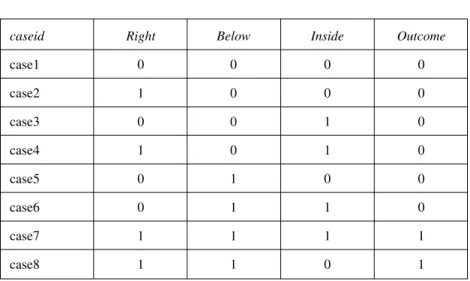
Because each condition divides the universe into two parts, the set of three conditions divides it in 2 * 2 * 2 = 8 zones, called “elementary zones.” Within each zone, the values for conditions of each case are the same. Let us also suppose that we know the value of the outcome variable for each one of these 8 zones. The data can first be presented in tabular format (see Table 3.1).
The first column of Table 3.1 contains the case labels (“caseid”), from “case1” to “case8.” The following three columns contain all logically possible combinations (there are 8 of them—i.e., 23
; see p. 27) of the binary RIGHT, BELOW, and INSIDE conditions. Finally, the fifth column contains the value of the OUTCOME for each one of the 8 combinations. The first six cases dis-play a [0] outcome (Boolean notation: [outcome]), while the last two disdis-play a [1] outcome (Boolean notation: [OUTCOME]). The Boolean expression that was minimized above (see Formulas 1 and 2 in Box 3.2.) corresponds simply to a translation of the two bottom rows of this table.
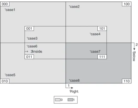
This same data can be represented in a visual way, in aVenn diagram(see also p. 23), showing visually that each condition cuts the universe of cases in two (Figure 3.1) and making the 8 basic zones visible.
In this Venn diagram:
• Condition [RIGHT] cuts the space vertically: All cases on the right-hand side of
the vertical line have a (1) value for this condition, whereas all cases on the left-hand side of this line (“not right”) have a (0) value for this condition.
• Condition [BELOW] cuts the space horizontally: All cases below the horizontal
line have a (1) value for this condition, whereas all cases above this line (“not below”) have a (0) value for this condition.
• Finally, condition [INSIDE] cuts the space between what’s inside or outside the
square in the middle: All cases inside the square have a (1) value for this condi-tion, whereas all cases outside the square (“not inside”) have a (0) value for this condition.
This Venn diagram also contains information about where each case is located. In this simple example, each basic zone is occupied by a single case. In addition, the diagram contains information about the value of the outcome variable. Let us consider only the [1] outcome. It corresponds to the dark-shaded area, at the bottom right of the diagram, and corresponds indeed to
caseid Right Below Inside Outcome
case1 0 0 0 0 case2 1 0 0 0 case3 0 0 1 0 case4 1 0 1 0 case5 0 1 0 0 case6 0 1 1 0 case7 1 1 1 1 case8 1 1 0 1
case7 and case8 (as in the last two lines of Table 3.1). This light shaded area can be expressed, in Boolean notation, as follows (Formula 3):
RIGHT * BELOW * INSIDE + RIGHT * BELOW * insideOUTCOME Note that this formula is exactly the same as Formula 1. It is read as follows: “The outcome is present for case7 [a case that is on the right AND below AND inside] OR for case8 [a case that is on the right AND below ANDnot inside].” This is a long formulation, which requires the description of each basic zone: It describes first the basic zone where case7 stands, then the one where case8 stands. Technically speaking, this formula contains twoterms(each term is a combination of conditions linked by the “AND” operator), and each term contains all three conditions. This is precisely where the Boolean minimiza-tion intervenes: It makes possible describing these two zones with one simpler and shorter expression, consisting of only oneterm.Indeed, we notice, visu-ally, that the two basic zones where cases 7 and 8 stand, when combined, form
000 3Inside Right B e lo w 1 2 0 1 100 110 010 011 001 101 111 ↓ .case1 .case2 .case4 .case7 .case3 .case6 .case5 .case8
Figure 3.1 Venn Diagram Corresponding to Table 3.1 (3 Condition Variables)*
a larger square: All the cases that are located below the horizontal line, AND all the cases that are located on the right-hand side of the vertical line. This larger zone can be expressed as (Formula 4):
RIGHT * BELOWOUTCOME
Note that this formula is exactly the same as Formula 2. It means that we simply need to know about two conditions—[RIGHT] and [BELOW]—to account for the outcome, which corresponds to cases 7 and 8. We need not know whether or not those cases are inside or “not inside” the middle square, because this information is superfluous: What is shared by these two cases with a [1] outcome is that they are “on the right AND below.” So we can simply remove the [INSIDE/not inside] condition.
As we shall see later, this is exactly the operation that is performed by the software on more complex data sets, with more conditions, and also with “empty” basic zones (i.e., with no cases observed). Of course, this makes the operations somewhat more complex, so it is best to let the computer perform the algorithms (in csQCA, the software uses the Quine minimization algorithm).
Now that we have introduced the basics of Boolean language and opera-tions, we can present key practical steps of csQCA. We shall pursue the same example as in Chapter 2, from the inter-war project, where the cases are 18 European countries.
S T E P 1 : B U I L D I N G A D I C H OTO M O U S DATA TA B L E
Of course, building a relevant data table requires previous work: A well-thought-out comparative research design, and in particular rigorous case and variable selection (see Chapter 2). Remember, also, that at this stage the researcher is supposed to have gained adequate substantive knowledge about each case and theoretical knowledge about the most relevant variables (condi-tions, in particular) included in the analysis.
Among the large variety of approaches dealing with the more general conditions favoring the emergence and consolidation of democratic political systems in different parts of the world (see p. 26: list of main categories of con-ditions in the inter-war project), we have selected one that addresses overall socioeconomic and “structural” factors. Of course, for a more comprehensive account other factors such as specific historical and cultural conditions, inter-mediate organizations, institutional arrangements, actor-related aspects, and so on must also be considered (for an application of such a more comprehensive
design, see also Berg-Schlosser, 1998). For purposes of illustration, however, using the selected approach will suffice—in short, for the sake of clarity, we need a relatively simplified theory, which does not entail too many conditions. As a reminder, the specific outcome we are trying to “explain” here is the sur-vival or breakdown of democratic systems in Europe during the inter-war period. Why is it that some democratic systems survived, while others collapsed? In QCA terminology, this variable we seek to explain is called theoutcome.
The most influential study dealing with the more general socioeconomic preconditions of democracy was S. M. Lipset’s Political Man (1960), in particular his chapter “Economic Development and Democracy.” There, he (re)stated the general hypothesis that “the more well-to-do a nation, the greater the chances that it will sustain democracy” (p. 31). Indeed, among the “stable European democracies” analyzed by Lipset were cases like Belgium, the Netherlands, Sweden, and Great Britain, which all showed high levels of wealth, industrialization, education, and urbanization. Under his (very broad) category of “unstable democracies and dictatorships” figured countries like Greece, Hungary, Italy, Poland, Portugal, and Spain, with lower levels in this regard. However, he also noted that
Germany is an example of a nation where growing industrialization, urbanization, wealth and education favoured the establishment of a democratic system, but in which a series of adverse historical events prevented democracy from securing legitimacy and thus weakened its ability to withstand crisis. (p. 20)
This statement certainly applies to Austria as well, but the kind of “adverse historical events” and their specific roots were not investigated by Lipset. Similarly, the fact that countries like Czechoslovakia, Finland, and France (which also had higher levels of development and democratic institutions, and which, as far as internal factors were concerned, survived the economic crisis of the 1930s) were grouped by Lipset in the same “unstable” category, was not very helpful from an analytical viewpoint. In later years, Lipset’s work was followed by a number of conceptually and statistically more refined studies and drew considerable criticism as well. However, when he later reviewed his original study, he still found its basic tenets confirmed (Lipset, 1994; see also Diamond, 1992).
For each of the four main dimensions discussed by Lipset (wealth, indus-trialization, education, and urbanization), we have selected one major indicator as listed in Table 3.2. and have provided the data for each one of the 18 cases (countries) considered.
In this example, we have 18 cases (each case being a row in Table 3.2). The outcome variable (SURVIVAL) is already of a dichotomous nature:
Table 3.2 Lipset’s Indicators, Raw Data (4 Conditions)
CASEID GNPCAP URBANIZA LITERACY INDLAB SURVIVAL
AUS 720 33.4 98 33.4 0 BEL 1098 60.5 94.4 48.9 1 CZE 586 69 95.9 37.4 1 EST 468 28.5 95 14 0 FIN 590 22 99.1 22 1 FRA 983 21.2 96.2 34.8 1 GER 795 56.5 98 40.4 0 GRE 390 31.1 59.2 28.1 0 HUN 424 36.3 85 21.6 0 IRE 662 25 95 14.5 1 ITA 517 31.4 72.1 29.6 0 NET 1008 78.8 99.9 39.3 1 POL 350 37 76.9 11.2 0 POR 320 15.3 38 23.1 0 ROM 331 21.9 61.8 12.2 0 SPA 367 43 55.6 25.5 0 SWE 897 34 99.9 32.3 1 UK 1038 74 99.9 49.9 1
Labels for conditions:
CASEID: Case identification (country name) abbreviations: AUS Austria; BEL Belgium; CZE Czechoslovakia; EST Estonia; FIN Finland; FRA France; GER Germany; GRE Greece; HUN Hungary; IRE Ireland; ITA Italy; NET Netherlands; POL Poland; POR Portugal; ROM Romania; SPA Spain; SWE Sweden; UK United Kingdom
GNPCAP: Gross National Product/Capita (ca. 1930)
URBANIZA: Urbanization (population in towns with 20,000 and more inhabitants) LITERACY: Literacy
INDLAB: Industrial Labor Force (including mining) (Details of sources in Berg-Schlosser & Mitchell, 2000, 2003.)
The [0] outcome value stands for “breakdown of democracy” (for 10 cases), and the [1] outcome value stands for “survival of democracy” (for the other 8 cases).
However, the four variables that are supposed to “explain” the outcome, which are calledconditions3in QCA terminology, are continuous
(interval-level) variables. To be used in csQCA, those original conditions must be dichotomized according to relevant thresholds.
To dichotomize conditions, it is best to use empirical (case-based) and the-oretical knowledge (see “good practices” box, below). In this example, we have chosen to set the dichotomization thresholds as follows4:
• [GNPCAP]: Gross National Product/Capita (ca. 1930): 0 if below 600 USD; 1 if
above.
• [URBANIZA]: Urbanization (population in towns with 20,000 and more
inhab-itants): 0 if below 50%; 1 if above.
• [LITERACY]: 0 if below 75%; 1 if above.
• [INDLAB]: Industrial Labor Force (incl. mining): 0 if below 30% of active
population; 1 if above.
• Always be transparent when justifying thresholds.
• It is best to justify the threshold on substantive and/or theoretical grounds. • If this is not possible, use technical criteria (e.g., considering the distribution of cases along a continuum; see also p. 79). As a last resort, some more mechanical cutoff points such as the mean or median can be used, but one should check whether this makes sense considering the distribution of the cases.5
• Avoid artificial cuts dividing cases with very similar values.
• More elaborate technical ways can also be used, such as clustering techniques (see p.130), but then you should evaluate to what extent the clusters make theoretical or empirical sense.
• No matter which technique or reasoning you use to dichotomize the conditions, make sure to code the conditions in the correct “direction,” so that their presence ([1] value) is theoretically expected to be associated with a positive outcome ([1] outcome value).
Box 3.3
“Good Practices” (3): How to Dichotomize Conditions in a Meaningful Way
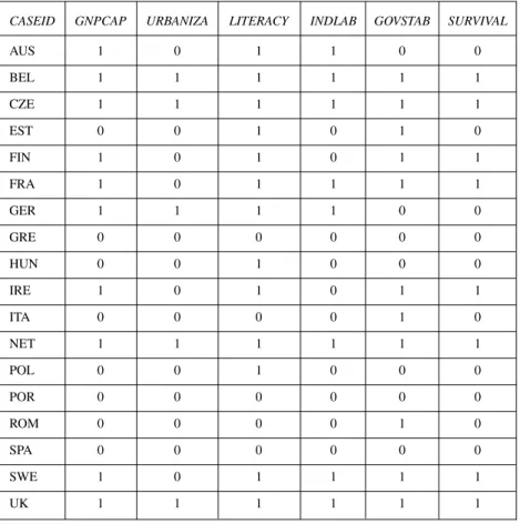
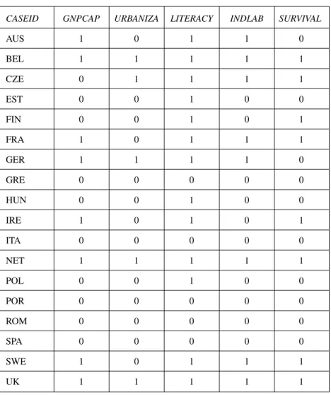
We thus obtain a dichotomized data table (Table 3.3). Already before engaging in csQCA proper, exploring this table visually, in a non-formal way, we can easily see that some cases corroborate very neatly the Lipset theory, by looking at the most extreme cases.
Table 3.3 Lipset’s Indicators, Dichotomized Data (4 Conditions)
CASEID GNPCAP URBANIZA LITERACY INDLAB SURVIVAL
AUS 1 0 1 1 0 BEL 1 1 1 1 1 CZE 0 1 1 1 1 EST 0 0 1 0 0 FIN 0 0 1 0 1 FRA 1 0 1 1 1 GER 1 1 1 1 0 GRE 0 0 0 0 0 HUN 0 0 1 0 0 IRE 1 0 1 0 1 ITA 0 0 0 0 0 NET 1 1 1 1 1 POL 0 0 1 0 0 POR 0 0 0 0 0 ROM 0 0 0 0 0 SPA 0 0 0 0 0 SWE 1 0 1 1 1 UK 1 1 1 1 1
For instance, Belgium (row 2) is a “perfect survivor case,” corroborating Lipset’s theory: A [1] value on all four conditions leads to the [1] outcome value [SURVIVAL]. Conversely, Portugal (row 14) is a “perfect breakdown case,” corroborating Lipset’s theory: A [0] value on all four conditions leads to the [0] outcome value [survival]. However, for many other cases, the picture looks more complex.
S T E P 2 : C O N S T RU C T I N G A “ T RU T H TA B L E ”
The first step for which we need csQCA proper (in terms of specific software treatment6
) corresponds to a first “synthesis” of the raw data table. The result thereof is called atruth table.It is atable of configurations—remember that a configuration is, simply, a given combination of conditions associated with a given outcome. There are five types of configurations, each of which may cor-respond to none, one, or more than one case.
• Configurations with a [1] outcome (among theobservedcases); also called “1configurations.”
• Configurations with a [0] outcome (among theobservedcases); also called “0 configurations.”
• Configurations with a “–” (“don’t care”) outcome (among the observed cases); also called “don’t care configurations.” It means that the outcome is indeterminate.This is to be avoided, since the researcher is supposed to be interested in explaining a specific outcome across well-selected cases.7 • Configurations with a « C » (« contradiction ») outcome, called
con-tradictory configurations.Such a configuration leads to a « 0 » outcome for some observed cases, but to a « 1 » outcome for other observed cases. This is a logical contradiction, which must be resolved (see p. 48) before engaging further in the csQCA.
• Finally, configurations with an “L” or “R” (“logical remainder”) outcome.These are logically possible combinations of conditions that have not been observed among the empirical cases.
Box 3.4
Five Types of Configurations
Table 3.4 displays the truth table corresponding to the dichotomized data in Table 3.3.
Table 3.4 Truth Table of the Boolean Configurations
CASEID GNPCAP URBANIZA LITERACY INDLAB SURVIVAL
SWE, 1 0 1 1 C FRA, AUS FIN, HUN, 0 0 1 0 C POL, EST BEL, NET, 1 1 1 1 C UK, GER CZE 0 1 1 1 1 ITA, ROM, 0 0 0 0 0 POR, SPA, GRE IRE 1 0 1 0 1
• Check again that there is a mix of cases with a “positive” outcome and cases with a “negative” outcome (see Box 2.2, good practices for the case selection). • Check that there are no counterintuitive configurations. In this example, these would be configurations in which all [0] condition values lead to a [1] outcome, or all [1] condition values lead to a [0] outcome. • Check for cross-condition diversity; in particular, make sure that some
conditions do not display exactly the same values across all cases; if they do, ask yourself whether those conditions are too “proximate” to one another (if they are, they can be merged).
• Check that there is enough variation for each condition (a general rule: at least1/3 of each value) (see also Box 2.3, good practices for condition selection: “a variable must vary”. . . ).
If one of these criteria is not met, reconsider your selection of cases and/or conditions or possibly the way you have defined and operationalized the outcome. It is also useful, at this stage, to check for the necessity and sufficiency of each condition with regard to the outcome.
Box 3.5
“Good Practices” (4):Things to Check to Assess the Quality of a Truth Table
This truth table (Table 3.4) shows only the configurations corresponding to the 18observedcases. It already allows us to “synthesize” the evidence sub-stantially, by transforming the 18 cases into 6 configurations. We find out the following:
• There are two distinct configurations with a [1] outcome, corresponding
respec-tively to Czechoslovakia and Ireland.
• There is one configuration with a [0] outcome, corresponding to five cases (Italy,
Romania, Portugal, Spain, and Greece). It fits quite neatly with the Lipset theory, because a [0] value for all four conditions leads to a [0] outcome (breakdown of democracy).
We also notice that there are 3contradictory configurations(the first 3 rows in the truth table), corresponding to no less than 11 cases out of the 18. In other words: Lipset’s theory—in the way we have operationalized it, at least—does not enable us to account for 11 out of 18 cases. The third contradictory configuration is particularly troubling: It contains [1] values on all of the con-ditions and yet produces the [0] outcome for one case (namely, Germany), whereas it produces the expected [1] outcome for the other 3 cases (Belgium, Great Britain, and the Netherlands).
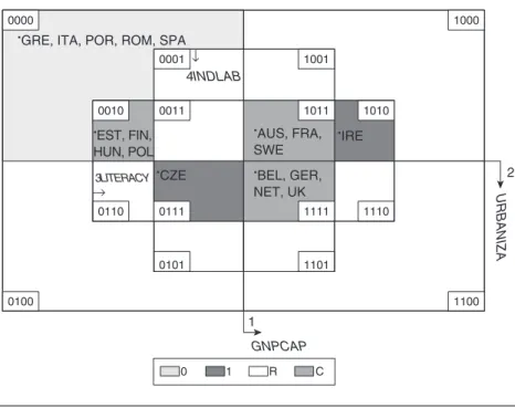
The data in this truth table can once again be visualized through a Venn dia-gram, a bit more complex than Figure 3.1 because it contains 4 conditions instead of 3 (Figure 3.2).
This Venn diagram has 16 basic zones (configurations)—that is, 24
zones. It is constructed using the same logic as Figure 3.1. In this empirically grounded example, we can observe four types of configurations:
• Two configurations with a [1] outcome, covering respectively the cases of
Czechoslovakia and Ireland.
• One configuration with a [0] outcome, covering the five cases of Italy, Romania,
Portugal, Spain, and Greece.
• Three contradictory configurations, covering in all 11 cases (the shaded zones
corresponding to the “C” label).
• Finally, many non-observed, “logical remainder” (“R”) configurations—10
alto-gether. Thus, there is limited diversity (see p. 27) in the data: As the 18 observed cases correspond to only 6 configurations, the remaining Boolean property space is devoid of cases. As will be shown at a later stage, these “logical remainder” configurations will constitute a useful resource for further analyses.
One way to look at this evidence, from a purely numerical perspective, would be to state that the model “fits” 7 out of 18 cases. This is, however, not a correct
way to proceed; remember that QCA is a case-oriented method (see p. 6), and that each case matters. From this perspective, it is a problem that so many con-tradictions occur. Hence these concon-tradictions first have to be resolved before pro-ceeding to the core of csQCA—namely, Boolean minimization.
At this stage of the analysis, it is also useful to check for the necessity and sufficiency of each condition with regard to the outcome. Let us assume a model that contains three conditions, A, B and C. For condition A, for instance, assessing itsconsistencyas a necessary condition means answering the following question: “To what extent is the statement ‘condition A is nec-essary for the outcome’ consistent?” Technically, this can be computed as follows: [the number of cases with a [1] value on the condition AND a [1] out-come value, divided by the total number of cases with a [1] outout-come value]. For more details, see Goertz (2006a), Ragin (2006b), and Schneider and Wagemann (2007, forthcoming). 0000 0110 0101 1101 1110 1000 1100 0100 3LITERACY 1 U R B A N IZ A 0 1 R C
.GRE, ITA, POR, ROM, SPA
.IRE .AUS, FRA,
SWE
.EST, FIN,
HUN, POL
.CZE .BEL, GER,
NET, UK 4INDLAB ↓ ↓ 0010 0011 1001 1010 1111 0111 0001 1011 GNPCAP 2
Figure 3.2 Venn Diagram Corresponding to Table 3.4 (4 Conditions)*
S T E P 3 : R E S O LV I N G C O N T R A D I C TO RY C O N F I G U R AT I O N S
It is perfectly normal to detect contradictory configurations in the course of a csQCA. It does not mean that the researcher has failed. Quite the contrary, contradictions tell us something about the cases we are studying. By seeking a resolution of these contradictions, the researcher will get a more thorough knowledge of the cases (through his or her “dialogue with the cases”), be forced to consider again his or her theoretical perspectives, and, eventually, obtain more coherent data. Remember that QCA techniques are best used in an iterative way (see p. 14). Thus addressing contradictions is simply part of this iterative process of “dialogue between ideas and evidence” (Ragin, 1987). Insofar as possible, all such contradictions should be resolved or, at least, one should strive to reduce contradictions as much as possible (Ragin, Berg-Schlosser, & De Meur, 1996, p. 758)—because, eventually, the cases involved in those contradictory configurations will be excluded8
from the analysis. Once again, this is problematic given the case-oriented nature of QCA.
There are basically eight strategies. In real-life research, it is advisable to at least consider all those strategies, and most often it will turn out that some combi-nation is useful.
1.Probably the easiest one: Simply add some condition(s) to the model. Indeed, the more complex the model—the more numerous the conditions—the less likely contradictions will occur, because each condition added constitutes a potential additional source of differentiation between the cases. Of course, such a strategy should not be pursued in a “hope-and-poke” way; it should be cautious and theoretically justified. It is advisable to add conditions one by one, not to obtain too complex a model. Otherwise, you run the risk of cre-ating a greater problem of “limited diversity” (see p. 27) and thus of “indi-vidualizing” explanations of each particular case; this means that csQCA will have missed its purpose of reaching some degree of parsimony (see p.10). 2. Remove one or more condition(s) from the model and replace it/them
by (an)other condition(s).
Box 3.6
“Good Practices” (5): How to Resolve Contradictory Configurations9
3. Reexamine the way in which the various conditions included in the model are operationalized. For instance, it may be that the threshold of dichotomization for a given condition is the source of the contradiction between two cases. By adjusting the threshold, it may be possible to resolve the contradiction. Alternatively, the contradiction could be due to data quality problems—in that case, one could collect complementary or revised data.This is the most labor-intensive option but very much to be advocated from a case-oriented perspective.
4. Reconsider the outcome variable itself.This strategy is often overlooked. If the outcome has been defined too broadly, it is quite logical that con-tradictions may occur. For instance, Rihoux (2001) noticed, during some exploratory csQCA analyses, that his initial outcome variable—major organizational change in a given political party—could in fact be decom-posed into two opdecom-posed subtypes: organizational adaptation and organi-zational radicalization. By focusing the outcome solely on organiorgani-zational adaptation, he was able to resolve many contradictory configurations. 5. Reexamine, in a more qualitative and “thick” way, the cases involved in each
specific contradictory configuration. What has been missed? What could differentiate those cases, that hasn’t been considered, either in the model or in the way the conditions or the outcome have been operationalized? 6. Reconsider whether all cases are indeed part of the same population (cf. case
selection, p. 20). For instance, if it is a “borderline” case that is creating the contradiction, perhaps this case should be excluded from the analysis. 7. Recode all contradictory configurations as [0] on the outcome value.This
solution, suggested by Ragin (1987), treats contradictory configurations as “unclear” and thus decides to accept fewer minimizable configurations in exchange for more consistency in the cases/outcome relationship. 8. Use frequency criteria to “orientate” the outcome. Let us consider a
contradictory configuration that involves nine cases. If, say, it leads to a [1] outcome for eight cases and to a [0] outcome for only one case, one could consider that the “most frequently traveled path” wins—thus the outcome would be considered as having a [1] value for all nine cases. Note, however, that this more probabilistic strategy is disputable from a “case-oriented” perspective.
Of course, the strategy(ies) chosen must be justified on empirical grounds (case-based knowledge) and/or on theoretical grounds and not be the result of some opportunistic “manipulation.”
If none of these strategies, or a combination thereof, resolves the contra-dictory configurations, some cases will have to be removed from the key min-imization procedure. In such an event, there are basically four options:
• Choose to move on and proceed with csQCA, even though there are still one or
more contradictory configuration(s) left. There are then two sub-options: Either delete the cases involved in the contradictions from the data table or keep them in the data table.10Those cases still involved in the contradictory configuration(s)
could then be interpreted separately (apart from the csQCA procedures proper), using a more qualitative-historical, case-specific approach.
• Consider using mvQCA or fsQCA (see Chapters 4 and 5), which are able to
process more fine-grained data. Indeed, the reason csQCA easily produces con-tradictions is simply because dichotomization strongly reduces the richness of the data and hence also masks potential differences across the cases (see p. 148: “costs” and “benefits” of dichotomization).
• Consider turning to other techniques, quantitative or qualitative. We recommend that
you at least try out mvQCA and/or fsQCA first (or in parallel, so you can weigh the strengths and limitations of the QCA techniques vis-à-vis the other techniques), because these two other QCA techniques will allow you to keep some key strengths of the QCA approach (both analytic and case-oriented, etc.—see Chapter 1).
• . . . or, if you are using csQCA for theory-testing, stop there and happily
con-clude that csQCA has allowed you to falsify the theory (see pp. 3, 16).
Technically speaking, if the decision is to proceed with csQCA, it is neces-sary to produce a revised dichotomized data table, which enables the software to produce a revised truth table. In real-life research, experience shows that several iterations may be necessary to obtain a contradiction-free truth table.
For this textbook example, we opt for the pragmatic way: Add a fifth con-dition to the model. In substance, we choose to add a “political–institutional” condition to the four more socioeconomic conditions derived from Lipset’s theory. This fifth condition is governmental stability (GOVSTAB). The thresh-old is placed as follows: A score of [0] (low stability) if 10 cabinets or more have governed during the period under investigation and a score of [1] (high stability) if fewer than 10 cabinets have governed during that same period.
The addition of this fifth condition can be justified on theoretical grounds: For the cases of “breakdown of democracy”: In the context of already less favorable socioeconomic circumstances, governmental instability further weakens the political system, the institutional capacity to address problems, and the credit of democratic institutions. Conversely, for the “survivors,” more stable governments are able to consolidate democratic institutions and enhance their capacity to confront political challenges.
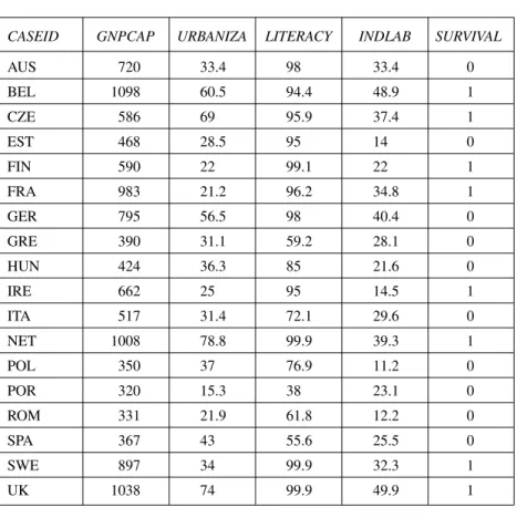
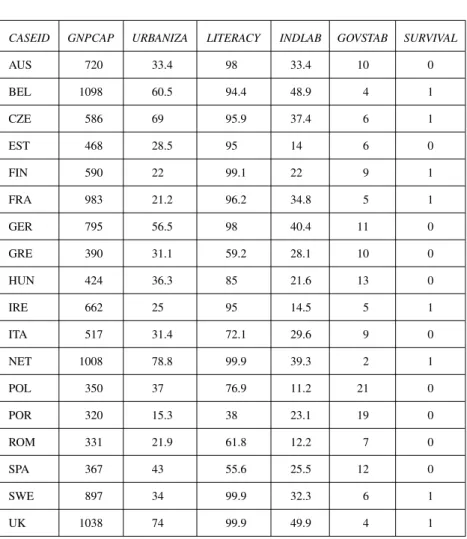
We thus obtain a new raw data table (Table 3.5, with one additional column as compared to Table 3.2), which is dichotomized (Table 3.6). The software then produces a new truth table (Table 3.7).
Table 3.5 Lipset’s Indicators, Raw Data, Plus a Fifth Condition
CASEID GNPCAP URBANIZA LITERACY INDLAB GOVSTAB SURVIVAL
AUS 720 33.4 98 33.4 10 0 BEL 1098 60.5 94.4 48.9 4 1 CZE 586 69 95.9 37.4 6 1 EST 468 28.5 95 14 6 0 FIN 590 22 99.1 22 9 1 FRA 983 21.2 96.2 34.8 5 1 GER 795 56.5 98 40.4 11 0 GRE 390 31.1 59.2 28.1 10 0 HUN 424 36.3 85 21.6 13 0 IRE 662 25 95 14.5 5 1 ITA 517 31.4 72.1 29.6 9 0 NET 1008 78.8 99.9 39.3 2 1 POL 350 37 76.9 11.2 21 0 POR 320 15.3 38 23.1 19 0 ROM 331 21.9 61.8 12.2 7 0 SPA 367 43 55.6 25.5 12 0 SWE 897 34 99.9 32.3 6 1 UK 1038 74 99.9 49.9 4 1
Labels for conditions: same as Table 3.2, plus a fifth condition: GOVSTAB: Governmental stability (number of cabinets in period) (Case abbreviations and sources: same as Table 3.2.)
This truth table (Table 3.7) is “richer” than the previous one (Table 3.4): By adding a condition, we move from 6 to 10 configurations, so indeed we have added diversity across the cases. This has enabled us to resolve most contra-dictions. Consider, for instance, the three cases of Austria, Sweden, and France, which formed a contradictory configuration when we considered only the four Lipset conditions (see first row in Table 3.4). By adding the [GOV-STAB] condition, we can now differentiate Austria (first row in Table 3.7), which has a [0] value on [GOVSTAB], from Sweden and France (fifth row in
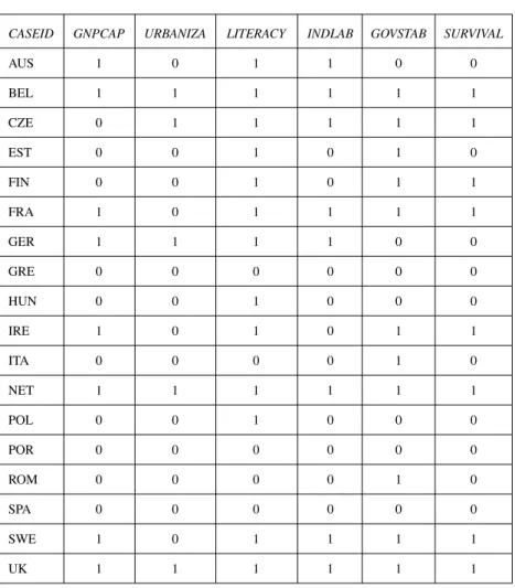
Table 3.6 Lipset’s Indicators, Dichotomized Data, Plus a Fifth Condition
CASEID GNPCAP URBANIZA LITERACY INDLAB GOVSTAB SURVIVAL
AUS 1 0 1 1 0 0 BEL 1 1 1 1 1 1 CZE 0 1 1 1 1 1 EST 0 0 1 0 1 0 FIN 0 0 1 0 1 1 FRA 1 0 1 1 1 1 GER 1 1 1 1 0 0 GRE 0 0 0 0 0 0 HUN 0 0 1 0 0 0 IRE 1 0 1 0 1 1 ITA 0 0 0 0 1 0 NET 1 1 1 1 1 1 POL 0 0 1 0 0 0 POR 0 0 0 0 0 0 ROM 0 0 0 0 1 0 SPA 0 0 0 0 0 0 SWE 1 0 1 1 1 1 UK 1 1 1 1 1 1
Table 3.7), which have a [1] value on [GOVSTAB]. Some other contradictions have been resolved in the same way.
However, there still is one contradictory configuration, embracing two cases: Estonia and Finland. Even with the addition of a fifth condition, those two cases still share the same values on all conditions, and yet they display different outcomes: Estonia is a “breakdown” case ([0] outcome), whereas Finland is a “survivor” case ([1] outcome). In such a situation, we now envis-age three possible options. The first one would be to further reexamine the model, which could—possibly—lead to the inclusion of a sixth condition (“good practice” strategy 1 in Box 3.6). The problem, however, is that the model becomes more complex with the addition of each condition and less clear for the pedagogical purpose of this textbook. The second option is simply to accept that those two cases deserve some specific qualitative-historical inter-pretation and that hence they should be left out for the next steps of the csQCA.
Table 3.7 Truth Table of the Boolean Configurations (4+1 Conditions)
CASEID GNPCAP URBANIZA LITERACY INDLAB GOVSTAB SURVIVAL
AUS 1 0 1 1 0 0 BEL, 1 1 1 1 1 1 NET, UK CZE 0 1 1 1 1 1 EST, FIN 0 0 1 0 1 C FRA, 1 0 1 1 1 1 SWE GER 1 1 1 1 0 0 GRE, 0 0 0 0 0 0 POR, SPA HUN, 0 0 1 0 0 0 POL IRE 1 0 1 0 1 1 ITA, 0 0 0 0 1 0 ROM
The third option (“good practice” strategy 3 in Box 3.6) is to reexamine the way in which the various conditions included in the model have been opera-tionalized, with a particular focus on the cases of Finland and Estonia. Doing this, we discover that if we move the threshold of the GNPCAP condition from $600 to $550 (actually this latter threshold is located near a natural “gap” in the data11), this allows us to differentiate between Finland ($590) and Estonia
($468). Incidentally, note that this modification of the threshold also changes the score for Czechoslovakia ($586: from a [0] to a [1] value). More impor-tant, it allows us to produce a contradiction-free truth table,12as is shown in
the next two tables (Tables 3.8 and 3.9).
Table 3.8 Lipset’s Indicators, Dichotomized Data, Plus a Fifth Condition (and GNPCAP Recoded)
CASEID GNPCAP URBANIZA LITERACY INDLAB GOVSTAB SURVIVAL
AUS 1 0 1 1 0 0 BEL 1 1 1 1 1 1 CZE 1 1 1 1 1 1 EST 0 0 1 0 1 0 FIN 1 0 1 0 1 1 FRA 1 0 1 1 1 1 GER 1 1 1 1 0 0 GRE 0 0 0 0 0 0 HUN 0 0 1 0 0 0 IRE 1 0 1 0 1 1 ITA 0 0 0 0 1 0 NET 1 1 1 1 1 1 POL 0 0 1 0 0 0 POR 0 0 0 0 0 0 ROM 0 0 0 0 1 0 SPA 0 0 0 0 0 0 SWE 1 0 1 1 1 1 UK 1 1 1 1 1 1
Table 3.9 can also be grasped more visually, through a Venn diagram (Figure 3.3). This five-dimensional diagram is a bit less easy to grasp than the previous, four-dimensional Venn diagram (Figure 3.2, above), but it is built on the same premises: Each condition still splits the logical space into two equal parts (of 16 basic zones each). Graphically, what is new is that the visualiza-tion of the fifth condivisualiza-tion (GOVSTAB) requires two separate “patches” (two horizontal squares, each one comprising 8 basic zones, in which this condition has a [1] value). Note also that many more basic zones of the logical property space are left empty (as compared with the previous, four-dimensional dia-gram; Figure 3.2)—a reminder that the more conditions we include in the model, the more limited the observed empirical diversity (see p. 27).
Indeed the revised, contradiction-free truth table (Table 3.9) now places Finland and Estonia in two separate configurations. More precisely: Estonia is now alone in a specific configuration, and Finland has joined Ireland in another configuration. Note also that Czechoslovakia has also moved and joined the
Table 3.9 Truth Table of the Boolean Configurations (4+1 Conditions, GNPCAP Recoded)
CASEID GNPCAP URBANIZA LITERACY INDLAB GOVSTAB SURVIVAL
AUS 1 0 1 1 0 0 BEL, 1 1 1 1 1 1 CZE, NET, UK EST 0 0 1 0 1 0 FRA, 1 0 1 1 1 1 SWE GER 1 1 1 1 0 0 GRE, 0 0 0 0 0 0 POR, SPA HUN, 0 0 1 0 0 0 POL FIN, IRE 1 0 1 0 1 1 ITA, 0 0 0 0 1 0 ROM
configuration of “perfect” survivor cases ([1] values on all conditions, leading to a [1] value on the outcome): Belgium, the Netherlands, and the UK.
S T E P 4 : B O O L E A N M I N I M I Z AT I O N
For this key operation of csQCA, the material used by the software is the truth table (Table 3.9) with its nine configurations: three configurations with a [1] out-come (corresponding to 8 cases), and six configurations with a [0] outout-come (cor-responding to 10 cases). As is obvious by looking at Table 3.9, each configuration may correspond to one or more empirical cases (or to none—the “logical remain-der” configurations; see p. 59). What is important to mention here is that the software does not recognize cases but rather theconfigurationsspecified in the truth table. Thus the number of cases in each configuration will not be relevant in the course of the minimization process. After the minimization, however, it will be possible to connect each of the cases to the minimal formula that is obtained.
10001 00010 10010 00011 00001 10011 00111 00101 00100 01110 01111 01101 01100 . ITA, ROM 4INDLAB 10101 10111 . FRA, SWE 00000 10000 .
GRE, POR, SPA
.
EST .FIN, IRE
. AUS . HUN, POL ↓ ↓ ↓ ↓ . GER . BEL, CZE, NET, UK 00110 10110 10100 11110 11100 11101 11111 11011 11001 01011 01001 01000 11000 11010 01010 3LITERACY GNPCAP U R B A N IZ A 0 1 R 5GOVSTAB 5GOVSTAB 2 1
Figure 3.3 Venn Diagram (5 Conditions; GNPCAP Recoded)*
The software minimizes these configurations, using the Boolean minimiza-tion algorithms (see Box 3.2), consideringseparatelythe [1] configurations and the [0] configurations. One must thus apply the minimization procedure twice, first for the [1] configurations, and then for the [0] configurations. The sequence is not important, as long as both are carried out. It is important to minimize both types of configurations, because we do not expect to find some form of perfect “causal symmetry” in social phenomena (see p. 9). In other words, we should not deduce the minimal formula for the [0] outcome from that of the [1] outcome, or vice versa, although it would be technically feasi-ble in some circumstances to do so by applying the De Morgan’s law.13
Minimization of the [1] Configurations (Without Logical Remainders)
First, we ask the software to minimize the [1] configurations,withoutincluding some non-observed cases. We obtain the following minimal formula (Formula 1):
GNPCAP * LITERACY * + GNPCAP * urbaniza * SURVIVAL INDLAB * GOVSTAB LITERACY * GOVSTAB
(BEL, CZE, NET, UK + (FIN, IRE + FRA, SWE) FRA, SWE)
This is called a “descriptive” formula, because it does not go much beyond the observed, empirical cases. In consists of twoterms, each one of which is a combination of conditions linked with the « 1 » outcome value. Following the Boolean notation (see Box 3.1), it can be read as follows:
“The ‘1’ outcome (survival of democracy) is observed:
• In countries that combine high GNP per capita [GNPCAP]ANDhigh literacy
rates [LITERACY]ANDhigh percentage of industrial labor forces [INDLAB]
ANDhigh governmental stability [GOVSTAB]
OR
• In countries that combine high GDP per capita [GNPCAP]ANDlow
urbaniza-tion [urbaniza]ANDhigh literacy rates [LITERACY]ANDhigh governmental stability [GOVSTAB]”
The firsttermof the minimal formula corresponds to six countries: on the one hand Belgium, Czechoslovakia, the Netherlands, and the UK (which share the same configuration—i.e., with all five conditions) and on the other hand14
France and Sweden. The second term corresponds to four countries: on the one hand Finland and Ireland and on the other hand France and Sweden. Note that concerning France and Sweden, we thus have two partly “concurrent” explanations. In such a situation—which is quite often met with csQCA—the researcher has to make a choice, using his or her case knowledge. This is part of the phase of interpretation of the minimal formula (see Step 6, p. 65).
This descriptive minimal formula is still quite complex, as each term still includes four out of the five conditions of the model. Only a small measure of parsimony has been achieved. The formula does allow some first interpreta-tions, however. For instance, we could interpret the fact that the [URBANIZA] condition does not play a role in the survival of democracy in Belgium, Czechoslovakia, the Netherlands, and the UK.
Note that the two terms of the formula share the [GNPCAP * LITERACY * GOVSTAB] combination of conditions. Thus, this combination can be made more visible by manually modifying the minimal formula (this is not done by the software). We simply treat the formula as a conventional algebraic expres-sion, a sum of products, and factor out the common conditions. This will pro-duce a more structured version of the formula—nota more parsimonious one, because no further conditions are eliminated by this operation. Thus, Formula 1 can be rewritten as follows (Formula 2):
INDLAB
GNPCAP * LITERACY * GOVSTAB *
{
SURVIVAL urbanizaThis rewriting of the formula shows quite clearly what is common to all the “survivor” cases (the left-hand side of Formula 2)—once again, this could be subject to interpretation by the researcher, as indeed this core combination of three conditions is shared by all “survivor” cases. The rewritten formula also shows what is specific to each one of the two clusters of cases (the two differ-ent “paths” on the right-hand side of Formula 2).
Minimization of the [0] Configurations (Without Logical Remainders)
Secondly, we perform exactly the same procedure, this time for the [0] con-figurations and also without including some non-observed cases. We obtain the following minimal formula (Formula 3):
gnpcap * urbaniza * indlab + GNPCAP * LITERACY * survival (EST + GRE, POR, SPA + INDLAB * govstab
HUN, POL + ITA, ROM) (AUS + GER)
As the previous one, this minimal formula is also quite complex. Reading this formula (following the same conventions as explained above), we see that csQCA provides us with two “paths” to the [0] outcome. The first one corre-sponds to many cases: Estonia; Greece, Portugal, and Spain; Hungary and Poland; Italy and Romania. These eight cases of democracy breakdown all share the [gnpcap * urbaniza * indlab] combination—i.e., the combination [0] values on three conditions—which is quite consistent with the theory. The second one is specific to Austria and Germany—note that this result could have been guessed by looking at the Venn diagram (Figure 3.3, p. 56), in which those two cases are “distant” from the eight above-mentioned cases. This formula cannot be rewritten in a “shorthand” manner, because the twotermshave noth-ing in common.
S T E P 5 : B R I N G I N G I N T H E “ L O G I C A L R E M A I N D E R S ” C A S E S
Why Logical Remainders Are Useful
The problem with Formulas 1 to 3 is that they are still quite complex: Relatively little parsimony has been achieved. To achieve more parsimony, it is necessary to allow the software to include non-observed cases, called “log-ical remainders.” In this example, remember that there is a large “reservoir” of logical remainders, as is seen in the Venn diagram (Figure 3.3, p. 56). Only a tiny proportion of the logical property space is occupied by empirical cases: Out of the 32 potential configurations (= 25, as there are 5 conditions; see p. 27),
only 9 correspond to observed cases. Thus, the 23 logical remainders (= 32 minus 9) constitute a pool of potential cases that can be used by the software to produce a more parsimonious minimal formula.
Why does the inclusion of logical remainders produce more parsimonious minimal formulas? This can be explained visually, using the Venn diagram and eight concrete cases: all those cases with a [0] outcome, which also happen to be situated on the left-hand side of the Venn diagram (Estonia; Greece, Portugal and Spain; Hungary and Poland; Italy and Romania).
First, note that the simpler (the “shorter”) a Boolean expression, the larger the number of configurations it covers:
• A combination of all five conditions covers only one configuration (e.g., the
[00000] zone, which contains the Greece, Portugal, and Spain cases).
• A combination of four conditions covers two configurations: If we want to
“cover” not only the Greece, Portugal, and Spain cases but also the zone right near it that contains the Italy and Romania cases (the [00001] zone), we only need to have information about four conditions. Indeed, we don’t need to know about the [GOVSTAB] condition: It has a [1] value for the Italy and Romania cases and a [0] value for the Greece, Portugal, and Spain cases.
• Likewise, a combination of three conditions covers four configurations. • A combination of two conditions covers eight configurations.
• And a statement containing only 1 condition covers 16 configurations—i.e., half
of the Boolean property space. For instance, the zone corresponding to a [0] value on the [GNPCAP] condition is the whole left half of the Venn diagram, corresponding to 16 configurations (only 4 of which, incidentally, contain some observed cases—those 8 cases that all happen to have a [0] outcome).
Following this logic, the usefulness of logical remainders is quite straight-forward: To express those eight cases in a simpler way, it suffices to express them as part of a broader zone, also comprising some logical remainders.
Hence what we can do is to make a “simplifying assumption” regarding the 12 logical remainders on the left-hand side of the Venn diagram: Let usassumethat, if they existed, they would also have a [0] outcome, just like the 8 observed cases. If this assumption is correct, then we have produced a much larger zone (the whole left-hand side of the Venn diagram, comprising 16 configurations) sharing the [0] outcome, and thus the 8 observed cases can be expressed in a much more parsi-monious way: simply [gnpcap]—i.e., [0] value for the [GNPCAP] condition.
This is exactly what the software does: It selectssomelogical remainders (only those that are useful to obtain a shorter minimal formula), adds them to the set of observed cases, and makes “simplifying assumptions” regarding these logical remainders. This then produces a simplertermin the minimal formula.
Minimization of the [1] Outcome (With Logical Remainders)
Running again the minimization procedure, this time allowing the software to include some of the logical remainders, we obtain the following minimal formula (Formula 4):
GNPCAP * GOVSTABSURVIVAL
It is read as follows: “For all these countries, a high GDP per capita, com-bined with governmental stability, has led to the survival of democracies in the inter-war period.” Comparing this formula with Formula 1 (see p. 57), we see that a more parsimonious solution has been achieved, thanks to the simplify-ing assumptions made by the software regardsimplify-ing some of the logical remain-ders. We can obtain a list of these simplifying assumptions from the software and lay them out in the report of the analysis—in this instance five of them were used15: 1/ GNPCAP{1}URBANIZA{0}LITERACY{0}INDLAB{0}GOVSTAB{1} 2/ GNPCAP{1}URBANIZA{0}LITERACY{0}INDLAB{1}GOVSTAB{1} 3/ GNPCAP{1}URBANIZA{1}LITERACY{0}INDLAB{0}GOVSTAB{1} 4/ GNPCAP{1}URBANIZA{1}LITERACY{0}INDLAB{1}GOVSTAB{1} 5/ GNPCAP{1}URBANIZA{1}LITERACY{1}INDLAB{0}GOVSTAB{1} These simplifying assumptions can be visualized in the Venn diagram (through the TOSMANA software). In Figure 3.4, the minimal formula (the “solution”) is represented by the horizontal stripes. This area corresponds to the three configurations with observed cases displaying a [1] outcome, plus five logical remainder configurations.
Minimization of the [0] Outcome (With Logical Remainders)
Likewise, we obtain the following minimal formula (Formula 5):
gnpcap + govstab survival
(EST + GRE, POR, SPA + (AUS + GER + GRE, POR, HUN, POL + ITA, ROM) SPA + HUN, POL)
It is read as follows:
• “In eight countries (Estonia, . . . and Romania), low GNP per capita ‘explains’
the breakdown of democracy in the inter-war period.
• In seven countries (Austria, . . . and Poland), governmental instability ‘explains’
the breakdown of democracy in the inter-war period.”
There are thus two alternative paths toward the [0] outcome. Note that for five countries (Greece, Portugal, and Spain; Hungary and Poland), both paths
are valid. In such a situation, the researcher must choose, country by country, and relying on his or her case knowledge, which path makes more sense.
Comparing this formula with Formula 2 (see p. 58), we see that substantial parsimony—even more16
than in Formula 4—has been gained, thanks to the “simplifying assumptions” made, by the software, regarding some of the log-ical remainders. We can also obtain a list of these simplifying assumptions and lay them out in the report of the analysis. In this case, many more have been used (18 in all). This can be visualized through a Venn diagram (Figure 3.5; same conventions as Figure 3.4).
Examining Figures 3.4 and 3.5, it is clear that the minimal formula for the [0] outcome (including 18 logical remainders) and the minimal formula for the [1] outcome (including five logical remainders) are the perfect logical complementof one another. In other words, the software has used up all the available “empty space” of logical remainders, so as to produce the most
10000 10001 10101 10100 00010 10010 00011 00001 10011 00111 00110 00101 00100 11110 01110 01111 01011 01010 01100 01101 01001 01000 11111 11011 11001 11000 11010 11101 11100 3LITERACY . ITA, ROM .
GRE, POR, SPA
.
EST .FRA, SWE .FIN, IRE . AUS . GER . HUN, POL .
BEL, CZE, NET, UK 4INDLAB ↓ ↓ ↓ ↓ 00000 U R B A N IZ A GNPCAP 0 1 R 5GOVSTAB 5GOVSTAB 10111 10110 2 1
Figure 3.4 Venn Diagram: Solution for the [1] Outcome (With Logical Remainders)*
parsimonious minimal formulas possible. Thus, the two minimal formulas completely fill up the Boolean property space, well beyond the observed cases. This use of logical remainders raises a concern and also an important tech-nical issue. First the concern: Isn’t it altogether audacious to make assump-tions about non-observed cases? One way to frame this debate is to question the relative plausibility of those simplifying assumptions. This issue is addressed in detail in Ragin and Sonnett (2004; see also Ragin, 2008), in our review of the critiques of QCA (see p. 152) and of applications (see p. 135), and is exemplified in the fsQCA application below (see pp. 110–118). For reasons of space, we cannot engage here in a full discussion of this issue, using this inter-war project data. The key point to remember is that it is always possible torestrictthe choice of logical remainders used by the software. If we do this, we obtain somewhat less parsimonious minimal formulas.
01100 01110 01001 01101 01011 01111 01010 01001 11011 11001 5GOVSTAB 00001 00101 00100 00111 00110 10010 10101 11111 11101 3LITERACY 5GOVSTAB GNPCAP U R B A N IZ A 0 1 R .ITA, ROM .GRE, POR, SPA
.EST .FRA, SWE .FIN, IRE
.AUS
.GER .HUN, POL
.BEL, CZE, NET,
UK 4INDLAB ↓ Minimizing: 0 Including: R 00000 00010 00011 10100 10110 11110 11100 10001 10011 10111 11010 11000 1 2 10000
Figure 3.5 Venn Diagram: Solution for the [0] Outcome (With Logical Remainders)*
Second, the issue: What if the software uses thesamelogical remainders both for the minimization of the [1] configurations and for the minimization of the [0] configurations? If it does, it will produce “contradictory simplifying assumptions,” because indeed it would be a logical contradiction to assume that a given (non-observed) case would simultaneously have a [1] outcomeanda [0] outcome. Gladly, in this example, it is not the case. The comparison of Figures 3.4 and 3.5 shows that the two minimal formulas (with logical remainders) do not overlap. If we had encountered such a difficulty, it would have been possible to address it, using more advanced technical steps (see p. 136).
Finally, note that it is useful at this stage to assess thecoverageof the min-imal formulas—that is, the way the respective terms (or “paths”) of the minimal formulas “cover” the observed cases. This is a second measure of the “fit” of the model, as the measure of consistency (see p. 47) at a previous stage. Technically, one should make three measures, both for the [1] and [0] outcome values. For instance, for the [1] outcome value: (a)raw coverage:the proportion of [1] outcome cases that are covered by a given term; (b)unique coverage:the proportion of [1] outcome cases that are uniquely covered by a given term (no other terms cover those cases); (c)solution coverage:the pro-portion of cases that are covered by all the terms.17
Checklist for the minimization procedure(s), using the computer software:
• Perform the minimization both with and without inclusion of logical remainders. Each of these approaches may yield information of some interest. • Thus: Four complete minimization procedures must be run:
[1] configurations, without logical remainders [1] configurations, with logical remainders [0] configurations, without logical remainders [0] configurations, with logical remainders
• Ask the software to list the “simplifying assumptions” and display those in your research report.
• Check for possible “contradictory simplifying assumptions” and, insofar as possible, solve them (see p.136).
Box 3.7
“Good Practices” (6): Four Complete Minimization Procedures to Be Run and Made Explicit
S T E P 6 : I N T E R P R E TAT I O N
Remember that, as a formal data analysis technique, but even more so because it is a “case-oriented” technique (see p. 6), csQCA (the formal, computer-run part of it), as well as the other QCA techniques, is not an end in itself; rather, it is a tool to enhance our comparative knowledge about cases in small- and intermediate-N research designs.
This means that the final step of the procedure is a crucial one: The researcher interprets the minimal formulas. The emphasis can be laid more on theory or on the cases, or on both, depending on the research goals. Obviously this requires a “return to the cases” using the minimal formula(s) that is (are) considered most relevant. In the inter-war project example we have unfolded in this chapter, some case-based interpretations could follow from questions such as the following: What is the “narrative” behind the fact that, according to the minimal formula, high GNP per capita combined with governmental stability has lead to survival (or non-breakdown) of democracy in countries such as Belgium, Czechoslovakia, the Netherlands, and the UK? Is the “causal” story the same in these four countries? What distinguishes them from other countries also covered by this same minimal formula, such as France and Sweden? Why does low GNP per capita, as a single factor, seem to play a more prominent role in the breakdown of democracy in countries such as Estonia, Italy, and Romania? Conversely, why does a more directly “political” factor (governmental instability) come out as the single key determinant in democ-racy breakdown in countries such as Greece, Portugal, and Spain, even though these are also relatively poor countries (low GNP per capita as well)? To what extent is the “narrative” behind the German and Austrian cases of democracy breakdown really comparable? And so on.
To sum up: csQCA minimal formulas allow the researcher to ask more focused “causal” questions about ingredients and mechanisms producing
• Present all your minimal formulas (including the case labels), and if needed use visual displays (e.g., Venn diagrams) to make the minimal formulas more understandable for the reader.
• If it is useful for your interpretation, factor (by hand) some conditions, to make the key regularities in the minimal formulas more apparent.
• Assess the “coverage” of the minimal formulas—i.e., the connection between the respective terms of the minimal formulas and the observed cases.
(or not) an outcome of interest, with an eye on both within-case narratives and cross-case patterns. Note that unless individual conditions can be clearly sin-gled out (e.g., the condition is clearly a necessary condition or comes close to being a necessary and sufficient condition), it is important to refrain from interpreting relations between singular conditions and the outcome. At the interpretation stage, do not lose sight of the fact that the richness of csQCA minimal formulas resides precisely in the combinations and “intersections” of conditions. It would be a pity to lose a chance to gain some “configurational knowledge” (Nomiya, 2004) at this crucial stage. Note, finally, that these rules and ‘good practices’ of interpretation also apply to mvQCA and fsQCA.
• csQCA is based on a specific language, Boolean algebra, which uses only binary data ([0] or [1]) and is based on a few simple logical operations. As any language, its conventions must be properly used. It is a formal, but non-statistical, language.
• It is important to follow a sequence of steps, from the construction of a binary data table to the final “minimal formulas.”
• Two key challenges in this sequence, before running the minimization procedure, are: (1) implementing a useful and meaningful dichotomi-zation of each variable and (2) obtaining a “truth table” (table of configurations) that is free of “contradictory configurations.” • The key csQCA procedure is “Boolean minimization.” One must run the
minimization procedures both for the [1] and the [0] outcomes, and both with and without “logical remainders” (non-observed cases). • The use of “logical remainders”—and the “simplifying assumptions” that
are made on them by the software—raises some principal and technical difficulties, but the latter can be addressed.
• Obtaining minimal formulas is only the end of the computer-aided part of csQCA. It marks the beginning of a key final step: case- and/or theory-informedinterpretation, which should be focused on the link between key combinationsof conditions and the outcome.
Key Complementary Readings
Caramani (2008), De Meur & Rihoux (2002), Ragin (1987, 2000), Schneider & Wagemann (2007, forthcoming).
N OT E S
1. Note that, in most publications so far, the equal symbol [=] has been used. Following Schneider and Wagemann’s (2007) suggestion, we recommend using the arrow symbol [] instead. One of the key reasons therefore is that, by using this sym-bol, the Boolean formula can not be mistaken with a standard statistical (e.g., regres-sion) equation.
2. Actually, in this example, we can’t tell, because we should also examine the (combinations of) conditions leading to the absence ([0] value) of the outcome.
3. Acondition corresponds to an “independent variable” in statistical analysis. However, it is not an “independent” variable in the statistical sense. There is no assumption of independence between the conditions—quite the contrary; we would expect combinations to be relevant (see Chapter 1).
4. For more detailed justifications, see Berg-Schlosser and De Meur, 1994. 5. Typically, one should not use the median or the mean if this locates the dichotomization threshold in an area of the data distribution where many cases are situated (this would give opposite scores [0 or 1] to cases that display quite proximate raw values).
6. Actually the software (e.g., TOSMANA) can already be used in the prior stages—for example, for the clustering of cases (dichotomization) if one uses more technical criteria.
7. It is also a problem for further QCA software treatment. Each time the software meets a “don’t care” configuration, it will producetwo distinct configurations: one with a [0] outcome and one with a [1] outcome. This might not make sense from an empir-ical perspective. In practice, the “don’t care” outcome is rarely used, and even then it is used simply to signal a combination of conditions that is empirically impossible (e.g., pregnant males).
8. It is actually more complex—depending on whether or not the cases involved in those contradictory configurations are left (by the researcher) in the data table, this will have an impact on the size of the “reservoir” of non-observed “logical remainder” cases that can be used by the software in the minimization procedure (see note 10, below).
9. See also further discussion on p. 132.
10. Note that if one chooses to include logical remainders, these two sub-options will have a different influence on the end result (the minimal formula). If the cases involved in contradictions are deleted outright, the logical space they used to occupy will be left “open,” and the software will have the possibility to use this “free space” in its search for useful logical remainders—this is likely to generate a shorter, more par-simonious minimal formula. Conversely, if one keeps those cases in the data table, the logical space will be “occupied” by those cases, and the reservoir of potential “logical remainders” will be a little more constrained—this is likely to generate a less parsimo-nious minimal formula. Probably it is advisable to prefer the second, more cautious option, because we cannot assume that the logical space occupied by these contradic-tory cases is “empty empirical space.”
11. This can be visualized using the “thresholdssetter” function in TOSMANA (see p. 79).
12. This key suggestion has been made by Svend-Erik Skaaning.
13. For many reasons, one of which being that social phenomena display limited diversity (for a more detailed discussion, see De Meur & Rihoux, 2002). See also pp. 8–10 on the issue of causal complexity. However, under some very specific circumstances, De Morgan’s law can be meaningfully applied (see Wagemann & Schneider, 2007, p. 26).
14. In the TOSMANA output, the “+” sign in between (groups of) cases separates cases with different configurations (in the truth table).
15. The notation used here is that of the TOSMANA software for simplifying assumptions. GNPCAP{1} simply means [1] value on the GNPCAP condition; and so on (see Box 4.1).
16. This is simply because even more logical remainders have been included by the software for the minimization procedure.
17. For more details, see Ragin (2006b, 2008), Goertz (2006b), and Schneider & Wagemann (2007, forthcoming). Note that this operation is also implemented in mvQCA and fsQCA.

![Table 3.7), which have a [1] value on [GOVSTAB]. Some other contradictions have been resolved in the same way.](https://thumb-us.123doks.com/thumbv2/123dok_us/1901938.2778337/21.717.128.595.185.591/table-value-govstab-contradictions-resolved-way.webp)