6D SLAM 3D Mapping Outdoor Environments

Outdoor Environments

Andreas Nüchter,

Kai Lingemann, and Joachim Hertzberg Institute of Computer Science

University of Osnabrück D-49069 Osnabrück, Germany e-mail: 兵nuechter兩lingemann兩hertzberg其 @informatik.uni-osnabrueck.de

Hartmut Surmann Fraunhofer Institute IAIS Schloss Birlinghoven

D-53754 Sankt Augustin, Germany e-mail: [email protected]

Received 21 December 2006; accepted 3 July 2007

6D SLAM共simultaneous localization and mapping兲or 6D concurrent localization and mapping of mobile robots considers six dimensions for the robot pose, namely, thex,y, andzcoordinates and the roll, yaw, and pitch angles. Robot motion and localization on natural surfaces, e.g., driving outdoor with a mobile robot, must regard these degrees of freedom. This paper presents a robotic mapping method based on locally consistent 3D laser range scans. Iterative Closest Point scan matching, combined with a heuristic for closed loop detection and a global relaxation method, results in a highly precise mapping system. A new strategy for fast data association, cachedkd-tree search, leads to feasible computing times. With no ground-truth data available for outdoor environments, point relations in maps are compared to numerical relations in uncalibrated aerial images in order to assess the metric validity of the resulting 3D maps. © 2007 Wiley Periodicals, Inc.

1.

INTRODUCTION

Automatic environment sensing and modeling is a fundamental scientific issue in robotics, since the availability of maps is essential for many robot tasks.

Manual mapping of environments is a hard and te-dious job: Thrun reports a time of about one week of hard work for creating a map of the museum in Bonn for the robot RHINO共Thrun, 1998兲. In particular, mo-bile systems with 3D laser scanners that

automati-• automati-• automati-• automati-• automati-• automati-• automati-• automati-• automati-• automati-• automati-• automati-• automati-• automati-• automati-• automati-• automati-•

• • • • • • • • • • • • • •

cally perform multiple steps such as scanning, gag-ing, and autonomous driving have the potential to greatly improve mapping.

Reliable 3D robotic mapping has an evident im-pact on safety, security, and rescue robotics. It enables rescue robots to build maps, which can be used by rescue workers to recover victims and precisely locate potential threats. As another example application, we showed in an earlier work the mapping of abandoned underground mines. Serious threats emanate from abandoned mines, such as structural shifts, which can cause the surface above to collapse, and ground water contamination 共Nüchter, Surmann, Lingemann, Hertzberg & Thrun, 2004兲. Other applications also benefit from automatic and precise 3D environment modeling, e.g., industrial automation, architecture, agriculture, the construction or maintenance of tun-nels, and factory design, facility management, urban and regional planning.

The robotic mapping problem is that of acquiring a spatial model of a robot’s environment. If the robot poses were known, the local sensor inputs of the ro-bot, i.e., local maps, could be registered into a com-mon coordinate system to create a map. Unfortu-nately, any mobile robot’s self-localization suffers from imprecision. Therefore, the structure of the local maps, e.g., of single scans, needs to be used to create a precise global map. Finally, robot poses in natural outdoor environments involve yaw, pitch, roll angles, and elevation, turning pose estimation as well as scan registration into a problem in six mathematical di-mensions.

This paper proposes algorithms that allow us to digitize large environments and solve the 6D SLAM

problem. In previous works we already presented our core 6D SLAM algorithm with global relaxation 共Surmann, Nüchter & Hertzberg 2003; Surmann, Nüchter, Lingermann & Hertzberg, 2004兲 and loop closing共Surmann et al., 2004兲. This paper’s contribu-tion is threefold: First, we present an octree-based matching heuristic that allows us to match scans with rudimentary starting guesses and detect closed loops. Second, we present a novel search procedure, namely cached kd-trees, exploiting iterative behavior of the ICP algorithm. It results in a significant speed-up. Fi-nally, the paper summarizes our previous work on 3D mapping and gives a complete view of our algo-rithms.

The paper is organized as follows: Section 2 de-scribes related work. Then we introduce our solution to the 6D SLAM problem. Section 4 describes our strategies to render the algorithms computationally feasible. Section 5 presents a brief description of the used hardware, experiment, and results. Finally, Sec-tion 6 concludes.

2.

RELATED WORK

One way to categorize mapping algorithms is by the map type. In general, the map can either be topologi-cal or metritopologi-cal. Metritopologi-cal maps represent explicit dis-tances of the environment. These maps can either be 2D, usually an upright projection, or 3D, i.e., a volu-metric environment map. Furthermore, SLAM ap-proaches can be classified by the number of degrees of freedom of the robot pose. A 3D pose estimate con-tains the共x,y兲-coordinate and a rotation␪, whereas a

Table I. Overview of the dimensionality of SLAM approaches. Bold: 2D maps. Not bold: 3D maps.

Sensor data

Dimensionality of pose representation

3D 6D

Planar 2D mapping Slice-wise 6D SLAM

2D 2D mapping of planar sonar and

laser scans. See共Thrun 2002兲for an overview

3D mapping using a precise localiza-tion, considering thex,y,z-position

and the roll yaw and pitch angle.

Planar 3D mapping Full 6D SLAM

3D 3D mapping using a planar

localiza-tion method and, e.g., an upward looking laser scanner or 3D scanner.

3D mapping using 3D laser scan-ners or共stereo兲cameras with pose estimates calculated from the sensor

6D pose estimate considers all degrees of freedom a rigid mobile robot can have, i.e., the 共x,y,z兲-coordinate and the roll, yaw, and pitch angles. Three-dimensional maps can be generated by three different techniques: First, a planar localization method combined with a 3D sensor; second, a precise 6D pose estimate combined with a 2D sensor; and third, a 3D sensor with a 6D localization method. Table I summarizes these mapping techniques in comparison with planar 2D mapping. In this paper we focus on 3D data and 6D localization, hence, on 6D SLAM.

2.1. Planar 2D Mapping

The state of the art for planar metric maps are proba-bilistic methods, where the robot has probaproba-bilistic motion models and uncertain perception models. By integrating these two distributions with, e.g., a Kal-man or particle filter, it is possible to localize the robot 共Smith, Self & Cheesemen, 1986; Leonard & Durrant-Whyte, 1991兲. Mapping is often an exten-sion to this estimation problem. Beside the robot pose, positions or landmarks are estimated. Closed loops, i.e., a second encounter of a previously visited area of the environment, play a special role here. Once detected, they enable the algorithms to bound the error by deforming the already mapped area such that a topologically consistent model is created. However, there is no guarantee for a correct model. Several strategies exist for solving SLAM. Thrun re-views 共Thrun, 2002兲 existing techniques, i.e., maxi-mum likelihood estimation共Frese & Hirzinger, 2001; Folkesson & Christensen, 2003兲, expectation maximi-zation 共Thrun, Burgard & Fox, 1997兲, extended Kal-man filter 共Dissanayake, Newman, Clark, Currant-Whyte & Csorba, 2001兲 or 共sparse extended兲 information filter 共Thrun et al., 2004兲. In addition to these methods, FastSLAM 共Thrun, Fox & Burgard, 2000兲, that approximates the posterior probabilities, i.e., robot poses, by particles, and the method of Lu/ Milios on the basis of IDC scan matching共Lu & Mil-ios, 1997兲, play an important role in 2D.

In principle, the probabilistic methods from pla-nar 2D mapping are extendable to 3D mapping with 6D pose estimates 共Weingarten & Siegwart, 2005兲. However, to our knowledge no reliable feature ex-traction nor a strategy for reducing the computa-tional costs of multi-hypothesis tracking, e.g., FastSLAM, that grows exponentially with the

de-grees of freedom, has been published. The qualita-tive shift in the complexity is due to the necessity to draw samples in each dimension.

2.2. 3D Mapping

Planar 3D Mapping. Instead of using 3D scanners, which yield consistent 3D scans in the first place, some groups have attempted to build 3D volumetric representations of environments with 2D laser range finders. Thrun et al. 共2000兲, Früh & Zakhor 共2001兲 and Zhao & Shibasaki共2001兲use two 2D laser scan-ners for acquiring 3D data. One scanner is mounted horizontally, the other vertically. The latter one grabs a vertical scan line which is transformed into 3D points based on the current 3D robot pose. Since the vertical scanner is not able to scan sides of objects, Zhao & Shibasaki 共2001兲 use two additional, verti-cally mounted 2D scanners, shifted by 45° to reduce occlusions. The horizontal scanner is used to com-pute the 3D robot pose. The precision of 3D data points depends, besides on the precision of the scan-ner, critically on that pose estimation.

Recently, different groups employ rotating SICK scanners for acquiring 3D data 共Kohlhepp, Walther & Steinhaus, 2003; Wulf, Arros, Christensen & Wag-ner, 2004兲. Wulf et al. 共2004兲 let the scanner rotate around the vertical axis. They acquire 3D data while moving, thus the quality of the resulting map cru-cially depends on the pose estimate that is given by inertial sensors, i.e., gyros. In addition, their SLAM algorithms do not consider all six degrees of free-dom.

Slice-wise 6D SLAM. Local 3D maps built by 2D laser scanners and 6D pose estimates are often used for mobile robot navigation. A well-known example is the grand challenge, where the Stanford racing team used this technique for high speed terrain classifica-tion 共Thrun, Montemerlo & Aron, 2006兲.

Similar to the planar 3D mapping case, the accu-racy of the resulting 3D map depends on the robot’s pose estimate. This cannot be accomplished with in-expensive sensors.

Full 6D SLAM. A few other groups use highly accu-rate, expensive 3D laser scanners 共Allen, Stamos, Gueorguiev, Gold & Blaer, 2001; Georgiev & Allen, 2004; Sequeira, Ng, Wolfart, Goncalves & Hogg, 1999兲. The RESOLV project aimed at modeling inte-riors for virtual reality and tele-presence共Sequeira et al., 1999兲. They used a RIEGL laser range finder on robots and the ICP algorithm for scan matching共Besl

& McKay, 1992兲. The AVENUE project develops a robot for modeling urban environments共Allen et al., 2001兲, using a CYRAX scanner and a feature-based scan matching approach for registering the 3D scans. However, in their recent work they do not use data of the laser scanner in the robot control architecture for localization 共Georgiev & Allen, 2004兲. Hebert’s group has reconstructed environments using the Zoller+ Fröhlich laser scanner and aims to build 3D models without initial position estimates, i.e., with-out odometry information 共Hebert, Deans, Huber, Nabbe & Vandapel, 2001兲. Recently, Magnusson and Duckett proposed a 3D scan alignment method that, in contrast to the previously mentioned research groups, does not use the ICP algorithm, but the nor-mal distribution transform instead 共Magnusson & Ducket, 2005兲.

Other Approaches. Other approaches use information from CCD-cameras that provide a view of the ro-bot’s environment 共Biber, Andreasson, Duckett & Schilling, 2004; Se, Lowe & Little, 2001兲. Neverthe-less, cameras are difficult to use in natural environ-ments with changing light conditions. Camera-based approaches to 3D robot vision, e.g., stereo cameras and structure from motion, have difficulties provid-ing reliable navigation and mappprovid-ing information for a mobile robot in real-time. Thus, some groups try to solve 3D modeling by using planar scanner based SLAM methods and cameras, e.g., in Biber et al. 共2004兲.

3.

RANGE IMAGE REGISTRATION AND ROBOT

RELOCALIZATION

Multiple 3D scans taken from different poses are nec-essary to digitalize environments without occlusions. To create a correct and consistent model, the scans have to be registered in one common coordinate sys-tem. If the robot carrying the 3D scanner were pre-cisely localized, the registration could be done based directly on the robot pose. However, due to the

im-precise robot sensors, self-localization is erroneous, so the geometric structure of overlapping 3D scans has to be considered for registration. As a by-product, successful registration of 3D scans relocalizes the ro-bot in 6D by providing the transformation to be ap-plied to the robot pose estimation at the recent scan point. In this manner, localization and scan registra-tion, i.e., mapping, are intertwined.

Our solution to the 6D SLAM problem is based on scan registration. We consider a mobile robot re-cording its odometry and scanning the environment in a stop-scan-go fashion. The alignment of two scans is done by the ICP algorithm 共Besl & McKay, 1992兲. However, ICP alone is not sufficient for solving the 6D SLAM problem. The following extensions with re-gards to flexibility and speed have been made to this end:

1. Extrapolate the odometry to all six degrees of freedom.

2. Calculate heuristic initial estimations for ICP scan matching based on this extrapolation.

3. Register the 3D scans into a common coordi-nate system using ICP.

4. If applicable, close the loop and distribute the error.

5. After all scans are taken, refine the model by global relaxation.

These extensions will be handled in the following subsections. Our algorithm maintains a single 6D ro-bot pose estimate. The extensions provide the basis for reliable mapping, as shown in the result section. Combining 3D ICP scan matching and 6D poses in a multi-hypotheses approach is not computationally feasible. The approach presented in this paper con-centrates on single loops.

In our SLAM framework robot poses are repre-sented in different contexts in one of three different ways; namely, first; by an OPENGL-style 4⫻4 matrix, with the robot positiont=共x,y,z兲and its orientations given as the orthonormal matrixR苸R3

or, second, the corresponding six-vector, consisting of the position and of the Euler angles,

P=共x,y,z,␪_x,␪_y,␪_z兲,

or, third, as position and quaternion共see Section 3.4 for details兲,

P=共t,q兲 withq=共q0,qx,qy,qz兲.

Note the bold-italic共P, vectors兲and bold共P, matrices兲

notation. The conversion between the representa-tions, i.e., Euler angles, matrix representarepresenta-tions, and quaternions, is done by standard algorithms共Matrix FAQ, 1997兲.

The reason for using different theoretically equivalent representations, is that they have different numerical problems, such as gimbal locks, in

differ-ent situations. In the context of odometry processing we use Euler angles, for scan alignment, rendering is-sues orthonormal matrices, and interpolation tasks quaternions. Converting the representation is more efficient than coping with the problems in one single representation.

3.1. Odometry Extrapolation

Since nearly all mobile robots have an odometer to measure traveled distances, our algorithm uses these measurements to calculate a first pose estimation. The odometry is extrapolated to six degrees of free-dom using previous registration matrices. We are us-ing a left-handed coordinate system, i.e., they coor-dinate represents elevation. Then the change of the robot pose ⌬P given the odometry information 共xodon ,znodo,␪yodo,n兲, 共xodon+1,znodo+1,␪yodo,n+1兲, and the registra-tion matrixR共␪x,n,␪y,n,␪z,n兲, is calculated by solving

Therefore, calculating ⌬P

=共⌬xn+1,⌬yn+1,⌬zn+1,⌬␪x,n+1,⌬␪y,n+1,⌬␪z,n+1兲 re-quires a matrix inversion. If n= 1, R共␪x,n,␪y,n,␪z,n兲 is set to the identity matrix. Finally, the 6D posePn+1is calculated by

P_n+1=⌬P·P_n 共1兲

using the poses’ matrix representations. Thus, the planar odometry is extrapolated in 6D to the 共x,z兲-plane defined by the last robot pose. Note that the values for y_n+1,␪_x,n+1, and␪_z,n+1are usually not equal 0, due to the matrix inversion.

3.2. Calculating Heuristic Initial Estimations for ICP Scan Matching

We use the following heuristic to compute an initial estimation for the following ICP scan matching. It allows us to match scans with rudimentary starting guesses, as given by odometry. The heuristic com-putes octree representations from the last acquired scan D共data set兲and the previously acquired scans M 共model set兲and aligns them. More precisely, the following steps are executed:

1. Generate an octree D_M for the nth 3D scan 共model setM兲.

2. Generate an octree D_D for the 共n+ 1兲th 3D scan 共data setD兲.

3. For each search depth d

苸关o共sStart兲, . . . ,o共sEnd兲兴in the octrees, based on a functiono共x兲returning the depth within the octree that corresponds to a given cube sizex, estimate a transformation ⌬Pbest=共t,R兲 as follows, using the0-vector as initial value of

⌬Pbest:

共a兲 Calculate a maximal displacement and rotation⌬Pmax, depending on the search depth d and currently best transforma-tion⌬Pbest:

⌬Pmax=共dmax−d+ 1兲c+⌬Pbest, for some constant displacement vectorc. 共b兲 For all discrete 6-tuples ⌬Pi 苸关−⌬Pmax,⌬Pmax兴 in the domain ⌬P =共x,y,z,␪_x,␪_y,␪_z兲, displace the octreeD_D by⌬P_i·⌬P·P_n. Evaluate the matching of the two octrees by counting the number of overlapping cubes and save the best transformation as⌬P_best.

Note:Step 3共b兲requires six nested loops, but the computational requirements are bounded by the coarse-to-fine strategy inherited from the octree pro-cessing. The size of the octree cubes decreases expo-nentially with increasing d. We start the algorithm with a cube size of 75 cm3 _{and stop when the cube} size falls below 10 cm3_{. Using these values, d}

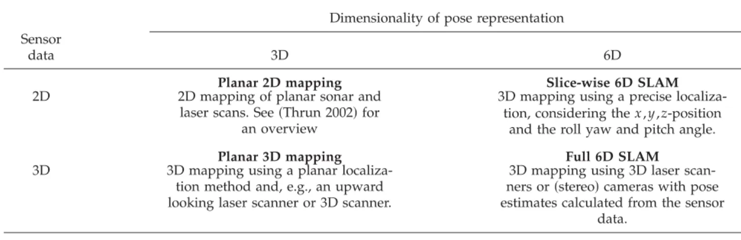
苸兵1 , . . . , 3其 in our experiments. Figure 1 shows two 3D scans and the corresponding octrees. Further-more, note that the heuristic works best outdoors. Due to the diversity of the environment, the match of octree cubes will show a significant maximum,

while indoor environments with their many geom-etry symmetries and similarities, e.g., in a corridor, are in danger of producing many plausible matches. To summarize, we used the following constants: sStart= 75 cm, sEnd= 10 cm, and c=共10, 10, 10, 5 , 10, 5兲 for quantifying the search windows, such that⌬Pmax decreases from iteration to iteration in each dimen-sion by the corresponding entry ofc. Finally,dmaxis the maximal depth of the tree. Informally spoken, the algorithm generates cube representations of each 3D scan共cf., Fig. 1兲. Then it searches for the optimal displacement that results in the maximum overlap of these cubes. In the next iteration the cube size is re-duced, i.e., cube representations given by a deeper level of the octree are utilized. Additionally, the size of the search interval is reduced with ongoing search depth/iteration.

After an initial starting guess is found, the range image registration, as described in the following sec-tion, proceeds with the robot pose estimation given as

共2兲 3.3. Scan Registration

The following method registers point sets into a common coordinate system. It is called ICP algo-rithm 共Besl & McKay, 1992兲. Given two indepen-dently acquired sets of 3D points, Mˆ and Dˆ, which correspond to a single shape, we aim to find the transformation consisting of a rotation R and a translation t which minimizes the following cost function:

Figure 1. Left: two 3D point clouds. Middle: octree corresponding to the black/front point cloud. Right: octree based on the gray/back points.

E共R,t兲=

兺

兺

The weights wi,jare assigned 1 if theith point ofM describes the same point in space as the jth point of D. Otherwise, wi,jis 0. Two things have to be calcu-lated: First, the corresponding points and, second, the transformation 共R,t兲 that minimizes E共R,t兲 on the base of the corresponding points.

The ICP algorithm calculates iteratively the point correspondences. In each iteration step, the al-gorithm selects the closest points as correspondences and calculates the transformation共R,t兲for minimiz-ing Eq.共3兲. In the last iteration step, the point corre-spondences are assumed to be correct. Figure 11 shows three frames of the alignment process. Besl & McKay共1992兲prove that the method terminates in a minimum. However, this theorem does not hold in our case since we use a maximum tolerable distance d_maxfor associating the scan data. Such a threshold is required though, given that 3D scans overlap only partially. Since the correct overlap is not known, us-ing a threshold d_maxresembles an estimation. Thus, the number of matched points in the iterations is not constant and Eq. 共3兲 does not decrease monotoni-cally.

In every iteration, the optimal transformation 共R,t兲has to be computed. Equation共3兲is reduced to

E共R,t兲⬀ 1 N

兺

N

储m_i−共Rd_f共m_i兲+t兲储2, 共4兲 withN=兩D兩=兺_i兩₌₁M兩兺_j兩D₌₁兩wi,jandD債Dˆ,M債Mˆ such that mi corresponds to df共m_i兲. The correspondences are

stored in a vector v=共共mi,df共m_i兲兲兲i containing the

point pairs, using a search functionf共mi兲that returns the index to a point in D with minimal distance to mi.

Four direct methods are known to minimize Eq. 共4兲 共Lorusso, Eggert & Fisher, 1995兲. In earlier work 共Surmann et al., 2003兲 we used a quaternion based method共Besl & McKay, 1992兲, but the following one, based on singular value decomposition共SVD兲, is ro-bust and easy to implement, thus we give a brief overview of the SVD-based algorithm. It was first published by Arun, Huang, & Blostein 共1987兲. The difficulty of this minimization problem is to enforce the orthonormality of the matrixR. The first step of the computation is to decouple the calculation of the

rotation Rfrom the translationtusing the centroids of the points belonging to the matching, i.e.,

cm= 1 N

兺

兺

⬘

⬘

⬘

⬘

After substituting共5兲and共6兲into the error function, Eq. 共4兲becomes

E共R,t兲⬀

兺

储m_i

⬘

⬘

R=VUT_{. Hereby, the matricesVandUare derived by} the singular value decompositionH=U⌳VT_{of a} cor-relation matrix H. This 3⫻3 matrixH is given by

H=

兺

⬘

⬘

冢

冣

with S_xx=兺_iN₌₁m_ix

⬘

⬘

⬘

⬘

We proposed and evaluated algorithms to accel-erate ICP, namely, point reduction and approximate kd-trees 共Nüchter et al., 2004; Surmann et al., 2003; Surmann et al., 2004兲, which are used here, too. They will be addressed in detail in Section 4.

3.4. Loop Closing

After registration, the scene has to be correct and globally consistent. The method just described for aligning several 3D scans is calledpairwise matching, i.e., the new scan is registered against a previous one. Alternatively, anincremental matchingmethod is used, where the new scan is registered against a so-calledmetascan, which is the union of the previously acquired and registered scans. Each scan matching has a limited precision. Both methods accumulate the registration errors such that the registration of a

large number of 3D scans leads to inconsistent scenes and to problems with the robot localization. Closing loop detection and error diffusing avoid these problems and compute consistent scenes. They are described next.

A loop is closed in SLAM if the robot returns to a pose close to one where a previous scan was taken. If the 3D scans where perfect and pairwise or incre-mental, matching would produce no errors. There would then be no need for matching the last against the first scan of a loop. In practice, matching errors accumulate leading to inconsistent maps.

Our algorithm automatically detects a

to-be-closed loop by registering the last acquired 3D scan with earlier acquired scans. Hereby we first create a hypothesis based on the maximum laser range and on the robot pose, so that the algorithm does not need to process all previous scans. Then we use the octree based method presented in Section 3.2 to re-vise the hypothesis. Finally, a loop is detected if reg-istration is possible, i.e., the number of closest points exceeds a certain threshold. The computed registra-tion error, i.e., the transformaregistra-tion 共R,t兲, is distrib-uted over all 3D scans in between. The respective part is weighted by the distance covered between the scans, i.e.,

ci=

length of the path from start of the loop to scan posei

overall length of the loop .

1. The translational part is calculated ast_i=c_it.

2. Of the three possibilities of representing ro-tations, namely, orthonormal matrices, quaternions and Euler angles, quaternions are best suited for our interpolation task. The problem with matrices is to enforce orthonor-mality and Euler angles show Gimbal locks 共Matrix FAQ, 1997兲. A quaternion as used in computer graphics is the 4 vectorq. Given a rotation as matrix R, the corresponding quaternionq is calculated as follows:

q=

冢

冣

冢

冑

冑

冑

冑

冣

with the elementsri,jofR. 共9兲 If trace 共R兲 共sum of the diagonal terms兲 is zero, the above calculation has to be altered:

Ifr_1,1⬎r_2,2andr_1,1⬎r_3,3then, q=

冢

冑

冑

冑

冑

冣

冢

冑

冑

冑

冑

冣

q=

冢

冑

冑

冑

冑

冣

The quaternion describes a rotation by an axis a苸R3_{and an angle␪ that are computed by}

a=

冢

冑

冑

冑

冣

The angle ␪ is distributed over all scans using the factor ci and the resulting matrix is derived as Matrix FAQ 共1997兲:

Ri=

冢

cos共ci␪兲+ax2共1 − cos共ci␪兲兲 azsin共ci␪兲+axay共1 − cos共ci␪兲兲 −aysin共ci␪兲+axaz共1 − cos共ci␪兲兲 −a_zsin共c_i␪兲+a_xa_y共1 − cos共c_i␪兲兲 cos共c_i␪兲+a_y2共1 − cos共ci␪兲兲 −axsin共ci␪兲+ayaz共1 − cos共ci␪兲兲 aysin共ci␪兲+axaz共1 − cos共ci␪兲兲 −axsin共ci␪兲+ayaz共1 − cos共ci␪兲兲 cos共ci␪兲+az2共1 − cos共ci␪兲兲

冣

. 共10兲

3.5. Model Refinement

Pulli presents a semi-automatic registration method that minimizes the global error and avoids inconsis-tent scenes共Pulli, 1999兲. The registration of one scan is followed by registering all neighboring scans such that the global error is distributed. Other matching approaches with global error minimization have been published, e.g.,共Benjemaa & Schmitt, 1997; Eg-gert, Fitzgibbon & Fisher, 1998兲. Benjemaa and Schmitt establish point-to-point correspondences first and then use randomized iterative registration on a set of surfaces. Eggert et al. compute motion updates, i.e., a transformation 共R,t兲, using force-based optimization, with data sets considered as connected by groups of springs.

Based on the idea of Pulli, we designed the re-laxation method simultaneous matching 共Surmann et al., 2003兲. The first scan is the master scan S₀ and determines the coordinate system. It is fixed. The fol-lowing three steps refine the model by minimizing the global scan matching error, after a queue is ini-tialized with the first scan of the closed loop共cf. Al-gorithm 1兲:

1. Pop the first 3D scan from the queue as the current one.

2. A set of neighbors共set of all scans that over-lap with the current scan兲is calculated. This set of neighbors forms one point setM. The current scan forms the data point setDand is aligned with the ICP algorithms if the current scan is not the master scanS0. One scan over-laps with another iff more thanp correspond-ing point pairs exist. In our implementation, p= 250.

3. If the current scan changes its location by ap-plying the transformation共translation or ro-tation兲 in step 2, e.g., the displacement is larger than 5 cm, then each single scan of the set of neighbors that is not in the queue is added to the end of the queue. If the queue is empty, terminate; else continue at step 1. In contrast to Pulli’s approach, our method is totally automatic and no interactive pairwise align-ment has to be done. Furthermore the point pairs are not fixed 共Pulli, 1999兲. Our algorithm, the function alignគscans共 兲 共line 11兲 recomputes the point

spondences, whereas Pullis algorithm uses corre-spondences established in an initialization step. The accumulated alignment error is spread over the whole set of acquired 3D scans. This diffuses the alignment error equally over the set of 3D scans 共Surmann et al., 2004兲.

Algorithm 1Model refinement

1: scanគqueue.push共Sclosedគloop兲 /* First scan of the closed loop *_/

2:whilescanគqueue⬅쏗do

3: Scurrent=scanគqueue. pop共 兲 4: metaគscan=쏗

5: fori= 0 tomaxគnumberគofគscansdo 6: p= numberគofគclosestគpoints共S_current,S_i兲

7: ifp艌250then 8: metaគscan.push共Si兲

9: end if

10: end for

11: 共⌬P, transformation兲= alignគscans共S_current,metaគscan兲

12: ifScurrent⬅S0then

13: apply transformation onS_current

14: end if

15: if⌬P⬎␧ then

16: scanគqueue=scanគqueue艛metaគscan

17: end if

18:end while

4.

PERFORMANCE ISSUES

The five steps in our SLAM algorithms have different computational costs. In our experiments, we acquire usually 3D scans with 20 000 up to 300 000 3D data points. While the first step共odometry extrapolation兲 is computed instantaneously, the octree based heuris-tic, applied naively, would need up to two seconds for calculating the two octrees and the rough align-ment of the scans. Since computing octrees is done in logarithmic time, the influence of larger data sets is negligible. The loop closing step共step four兲has simi-lar computational costs, since we use the octree heu-ristic again.

Most computational time is needed in the scan matching step 共step three兲 and in the model refine-ment共step five兲. While the model refinement can eas-ily be done offline, i.e., after the robot has finished the data acquisition, the scan matching is an essential part of the mapping procedure. We have a number of methods available to reduce significantly the

compu-tational costs, namely point reduction, kd-trees, ap-proximatekd-trees, and cachedkd-trees.

4.1. Point Reduction

Scanning is noisy and small errors may occur, namely, Gaussian noise and salt and pepper noise. The latter arises, for example, at edges where the laser beam of the scanner hits two surfaces, resulting in a mean and erroneous data value. Furthermore, reflections, e.g., at glass surfaces, lead to suspicious data. We propose two fast filtering methods to modify the data in order to enhance the quality of each scan.

The data reduction, used for reducing Gaussian noise, works as follows: The scanner emits the laser beams in a spherical way such that the data points close to the source are more dense. For point reduc-tion, multiple data points located close together 共Eu-clidian distance兲are replaced by their mean, using a standard reduction filter. The number of these so-called reduced points is one order of magnitude smaller than the original one.

For eliminating salt and pepper noise, a median filter removes the outliers by replacing a data point with the median value of the n surrounding points 共heren= 7兲. The neighbor points are determined ac-cording to their index within the scan, since the laser scanner provides the data in each scan slice sorted in a counter-clockwise direction. The median value is calculated with regard to the Euclidian distance of the data points to the point of origin. In order to remove noisy data but leave the remaining scan points untouched, the filtering algorithm replaces a data point with the corresponding median value if and only if the Euclidian distance between both is larger than a fixed threshold 共e.g., 200 cm兲.

Data reduction for the ICP algorithm is done us-ing the proposed filters. Without filterus-ing, a few out-liers may lead to multiple wrong point pairs during the 3D matching phase and results in an incorrect 3D scan alignment. Reduction and filtering are done in every single 2D scan slice while scanning, they are implemented as online algorithms and run in paral-lel to the 3D scan acquisition. In the end, the data for the scan matching is collected from every third scan slice. This fast vertical reduction yields a good sur-face description共cf. Fig. 2兲.

4.2. kd-trees

kd-trees are a generalization of binary search trees. Every node represents a partition of a point set to the two successor nodes. The root represents the whole point cloud and the leaves provide a com-plete disjunct partition of the points. These leaves are called buckets 共cf. Fig. 3兲. Furthermore, every node contains the limits of the represented point set.

4.2.1. Searchingkd-trees

Akd-tree is searched recursively for a closest point of a given query 3D point. The 3D point needs to be compared with the separating plane in order to de-cide on which side the search must continue. This procedure is executed until the leaves are reached.

There, the algorithm has to evaluate all bucket points. However, the closest point may be in a dif-ferent bucket, iff the distance to the limits is smaller than the one to the closest point in the bucket. In this case, backtracking has to be performed. Figure 3 shows a backtracking case, where the algorithm has to go back to the root. The test is known as ball-within-bounds test共Bentley, 1975; Friedman, Bentley & Finkel, 1977; Greenspan & Yurick, 2003兲.

4.2.2. The Optimizedkd-tree

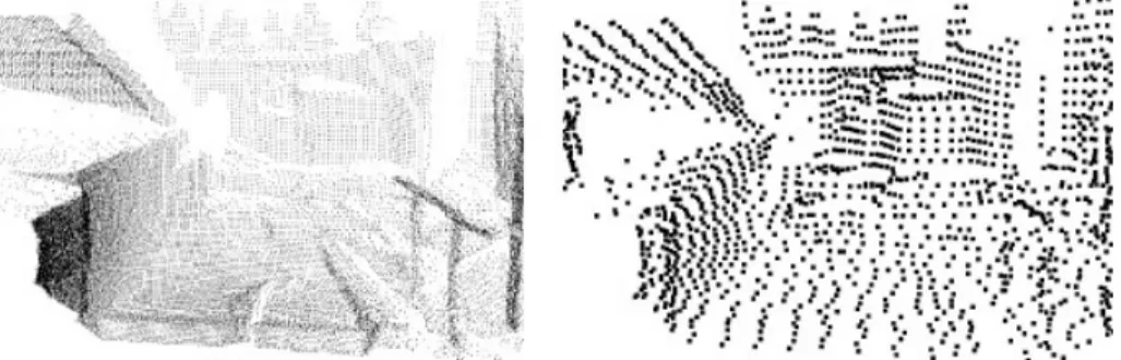
The objective of optimizingkd-trees is to reduce the expected number of visited leaves. Three parameters are adjustable, namely, the direction and position of the split axis as well as the maximal number of points in the buckets. Splitting the point set at the Figure 2. Left: a view of a 3D scene共66785 3D data points兲. Right: subsampled version共points have been enlarged, 6700 data points兲. To visualize the scanned 3D data, a viewer program has been implemented. The task of this program is to project a 3D scene to the image plane, i.e., the monitor, such that the data can be drawn and inspected from every perspective.

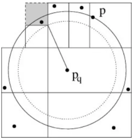
Figure 3. Left: recursive construction of akd-tree. If the query consists of pointpq,kd-tree search has to backtrack to the

tree root to find the closest point. Right: partitioning of a point cloud. Using the cut共b兲rather than共a兲results in a more compact partition and a smaller probability of backtracking共Friedman et al., 1977兲.

medianensures that everykd-tree entry has the same probability. The median can be found in linear time, thus computing the mean does not account for the time complexity of constructing the tree. Further-more, the split axis should be orientedperpendicular to the longest axis to minimize the amount of back-tracking共see Figure 3兲. Besides these results on com-plexity, Friedman and colleagues prove that a bucket size of 1 is optimal共Friedman et al., 1977兲. Neverthe-less, in practice it turned out that a slightly larger bucket size is faster.

4.3. Approximate kd-tree Search

Arya & D. Mount共1993兲introduce the following no-tion for approximating the nearest neighbor in

kd-trees: Given an ␧⬎0, then the pointp苸D is the 共1 +␧兲-approximate nearest neighbor of the pointp_q, if

储p−q储艋共1 +␧兲储p*_−q储,

where p* _{denotes the true nearest neighbor, i.e., p} has a maximal distance of ␧ to the true nearest neighbor共cf. Figure 4兲. Using this notation, in every step the algorithm records the closest point p. The search terminates if the distance to the unanalyzed leaves is larger than

储pq−p储/共1 +␧兲.

In the extreme case, thekd-tree does not implement any backtracking. To evaluate the quality of the scan matching, we acquired two 3D scans and measured the pose shift by a reference system, i.e., a meter rule. Figure 5 shows the starting poses from which a correct scan matching is possible. We conclude that the approximation does not influence the scan matching significantly, due to the large number of points used and the iterative nature of the algorithm. The running time of ICP scan matching decreases to roughly 75% in case of approximate kd-tree search. For a detailed evaluation see Nüchter, Lingemann, Hertzberg & Surmann, 共2005兲. However, the next method outperforms the approximatekd-tree search without the need of any approximation.

4.4. Cachedkd-trees

4.4.1. The Cachedkd-tree Search

kd-trees with caching contain, in addition to the lim-its of the represented point set and to the two child Figure 4. The 共1 +␧兲-approximate nearest neighbor. The

solid circle denotes the ␧ environment of pq. The search

algorithm need not analyze the gray cell, sincep satisfies the approximation criterion.关Figure adapted from共Arya & Mount, 1993兲兴.

Figure 5. The poses共x,z,␪y兲from which a correct alignment of two 3D scans is possible. Similar results for “matchable”

node pointers, one pointer to the predecessor node. The root node contains a null pointer. During the recursive construction of the tree, this information is available and no extra computations are required.

For the ICP algorithm, we distinguish between the first and the following iterations: In the first it-eration, a normal kd-tree search is used to compute the closest points. However, the return function of the tree is altered such that, in addition to the closest point, the pointer to the leaf containing the closest point is returned and stored in the vector of point pairs. This supplementary information forms the cache for future look-ups.

In the following iterations, these stored pointers are used to start the search. If the query point is located in the bucket, the bucket is searched and the ball-within-bounds test 共cf. Section 4.2.1兲 applied. Backtracking is started, if the ball lies not completely within the bucket. If the query point is not located within the bucket, then backtracking is also started. Since the search is started in the leaf node, explicit backtracking through the tree has to be implemented using the pointers to the predecessing nodes 共see Fig. 6兲. Algorithm 2 summarizes the ICP with cached kd-tree search.

Algorithm 2ICP with cachedkd-tree search

1:fori= 0 tomaxIterationsdo 2: ifi= 0then

3: for alldj苸Ddo

4: searchkd-tree of setMtop down for pointd_j

5: vi=共dj,mf共d_j兲, ptrគtoគbucket共mf共d_j兲兲兲

6: end for

7: else

8: for alld_j苸Ddo

9: searchkd-tree of setM, bottom up, for pointd_jusing ptrគtoគbucket共mf共d_j兲兲

10: v_i=共d_j,m_f共d

j兲, ptrគtoគbucketmf共dj兲兲

11: end for

12: end if

13 calculate transformation 共R,t兲 that minimizes the error function Eq.共4兲

14: apply transformation on data set D

15:end for

4.4.2. Performance of Cachedkd-tree Search

The proposed ICP variant uses exact closest point search. In contrast to the previously discussed ap-proximate kd-tree search for ICP algorithms 共Greenspan and Yurick, 2003; Nüchter et al., 2005兲, registration inaccuracies or errors due to approxima-tion cannot occur.

Friedman et al. 共1977兲 prove that searching for closest points usingkd-trees needs logarithmic time, i.e., the amount of backtracking is independent of the number of stored points in the tree. Since the ICP algorithm iterates the closest point search, the per-formance derives to O共I兩D兩log兩M兩兲, with I the num-ber of iterations. Note: Brute-force ICP algorithms have a performance ofO共I兩D兩兩M兩兲.

The proposed cached kd-tree search needs O共共I +兩M兩兲兩D兩兲time in the best case. This performance is reached if constant time is needed for backtracking, resulting in 兩D兩log兩M兩 time for constructing the tree, and I·兩D兩 for searching in case no backtracking is necessary. Obviously the backtracking time depends on the computed ICP transformation 共R,t兲. For small transformations the time is nearly constant.

Cached kd-tree search needs O共兩D兩兲 extra memory for the vectorv, i.e., for storing the pointers to the tree leaves. Furthermore, additional O共兩M兩兲 memory is needed for storing the backwards point-ers in the kd-tree.

Figure 6. Schematic description of the proposed search method: Instead of closest point searching from the root of the tree to the leaves that contain the data points, a pointer to the leaves is cached. In the second and following ICP iteration, the tree is searched backwards. The vector of point pairs memorizes the starting point of the search and, therefore, serves as a cache.

Figure 7 shows the following results of a de-tailed evaluation of the proposed cached kd-tree search algorithm:

1. The performance of the cachedkd-tree search depending on a change of the bucket size was tested: For small bucket sizes, the speed-up is larger共Figure 7, top left兲. This behavior origi-nates from the increasing time needed to search larger buckets.

2. The search time per iteration was recorded during the experiments共Figure 7, top right兲. For the first iteration the search times are equal, since cached kd-tree search uses con-ventional kd-tree search to create the cache. In the following iterations, the search time drops significantly and remains nearly con-stant. The conventional kd-tree search in-creases in speed, too. Here, the amount of

backtracking is reduced due to the fact that the calculated transformations共R,t兲are get-ting smaller.

3. The number of points to register influences the search time. With increasing number of points, the positive effect of caching algo-rithms becomes more and more significant 共Figure 7, bottom left兲.

4. The overall performance of the ICP algorithm depends both on the search time and on the construction time of the tree. However, the construction time of the trees seems to be negligible. In addition, a comparison with a reference implementation shows the effective implementation. As reference implementa-tion the software from the papers共Arya and Mount, 1993; Arya, Mount, Netanyahu, Sil-verman & Wu, 1998兲was used共Figure 7, bot-tom right兲.

Figure 7. Top left: achieved speedups of cachedkd-tree search compared to traditionalkd-tree search for an ICP based registration of two point sets. Top right: search time per iteration for bucket sizes 10 and 25. Bottom left: time consumption per ICP iteration. Bottom right: overall comparison of the algorithms and a referencekd-tree implementation共Arya and Mount, 1993兲.

5.

EXPERIMENTS AND RESULTS

5.1. Hardware Used in our Experiments

The 3D laser range finder is built on the basis of a SICK 2D range finder by extension with a mount and a small servomotor 共Figure 8兲 共Surmann et al., 2003兲. The 2D laser range finder is attached at the center of rotation to the mount for achieving a con-trolled pitch motion with a standard servo.

The area of up to 180°共h兲⫻120°共v兲 is scanned with different horizontal共181, 361, 721兲and vertical 共128, 225, 420, 500兲 resolutions. A plane with 181 data points is scanned in 13 ms by the 2D laser range finder 共rotating mirror device兲. Planes with more data points, e.g., 361, 721, duplicate, or qua-druplicate this time. Thus a scan with 181⫻256 data points needs 3.4 s. Scanning the environment with a mobile robot is done in a stop-scan-go fashion.

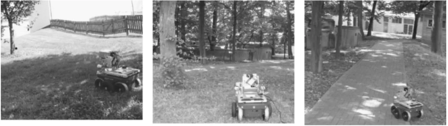
The mobile robot Kurt3D in its outdoor version 共Figure 8兲 is a mobile robot with a size of 45 cm 共length兲⫻33 cm 共width兲⫻29 cm 共height兲 and a weight of 22.6 kg. Two 90 W motors are used to power the six skid-steered wheels, whereas the front and rear wheels have no tread pattern to enhance rotating. The core of the robot is a Pentium-Centrino-1400 with 768 MB RAM and Linux. An em-bedded 16-bit CMOS microcontroller is used to con-trol the motor.

5.2. Full 6D SLAM in a planar environment

We applied the algorithms to a data set acquired at Schloss Dagstuhl. It contains 84 3D scans, each with

81225 共361⫻225兲, 3D data points, in a large, i.e., ⬃240 m, closed loop. The average distance between consecutive 3D scans was 2.5 m. Figure 9 shows the built 3D map.

We have also tested the algorithms on a 2D data set, computed from horizontal scan slices. This al-lows us to compare full 6D SLAM with planar 2D mapping共cf. Tab. I兲. Figure 10 shows the map. There are noticeable errors in the 2D alignment. The 2D scans do not provide enough structure for correct alignment. Many approaches bypass this problem by scanning the environment more often. However, the 3D data is much richer in information, therefore, 3D scan taken at sparse discrete locations are matched correctly共cf. Figure 9兲.

5.3. Full 6D SLAM in an Indoor/Outdoor Environment

The proposed algorithms have been applied to a data set acquired at the robotic lab in Birlinghoven. Thirty-two 3D scans, each containing 302 820 共721

⫻420兲range data points, were taken. The robot had to cope with a height difference between two build-ings of 1.05 meter, covered, on the one hand, by a sloped driveway in open outdoor terrain and, on the other hand, by a ramp of 12° inside the building. The 3D model was computed after acquiring all 3D scans.

Figures 11–13 show rendered 3D scans. The lat-ter figure presents the final model with the closed loop. Please refer to the website http:// kos.informatik.uni-osnabrueck.de/download/ 6Dpre/ for a computed animation and video through the scanned 3D scene.

In this data set, we analyzed the performance of the ICP scan matching. Details about this analysis can be found in共Surmann et al., 2004兲and共Nüchter, 2006兲. For ICP registration, the error tolerance for the initial estimation, i.e., the robot’s self localization, is about one meter in共x,y,z兲position and about 15° in the orientation. These conditions can be easily met using a cheap odometer and the presented heuristic for initial estimates for the ICP algorithm.

5.4. Full 6D SLAM in an Outdoor Environment The following experiment has been made at the campus of Schloss Birlinghoven with Kurt3D. Figure 14共left兲shows the scan point model of the first scans in top view, based on odometry only. The first part of the robot’s run, i.e., driving on asphalt, contains a systematic drift error, but driving on lawn shows more stochastic characteristics. The right part shows the first 62 scans, covering a path length of about

240 m. The heuristic described in Section 3.2 has been applied and the scans have been matched. The open loop is marked with a red rectangle.

At that point, the loop is detected and closed. More 3D scans have then been acquired and added to the map. Figure 15 共left and right兲 shows the model with and without global relaxation to visual-ize its effects. The relaxation is able to align the scans correctly even without explicitly closing the loop. The best visible difference is marked by a rectangle. The final map in Figure 15 contains 77 3D scans, each consisting of approx. 100 000 data points 共361

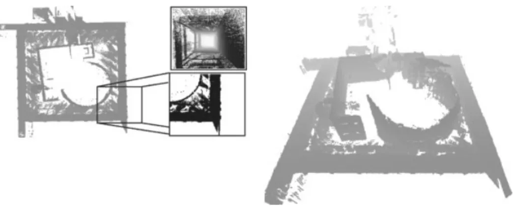
⫻275兲. Figure 16 shows two detailed views, before and after loop closing. The bottom part of Figure 15 displays an aerial view as ground truth for compari-son. Table II compares distances measured in the photo and in the 3D scene, at corresponding points 共taking roof overhangs into account兲. The lines in the photo have been measured in pixels, whereas real distances, i.e., the 共x,z兲-values of the points, have Figure 9. 3D digitalization of the International Conference and Research Center Schloss Dagstuhl. Left: 3D point cloud

共top view兲. Right: 3D view.

Figure 10. Two-dimensional digitalization of the environment with alignment problems at the wall on the right. Right: for comparison, the same closeup area of a horizontal slice from the generated 3D map共Figure 9兲.

been used in the point model. Considering that pixel distances in mid-resolution noncalibrated aerial im-age induce some error in ground truth, the corre-spondence show that the point model at least ap-proximates reality quite well.

Mapping would fail without first calculating the heuristic initial estimations for ICP scan matching, since ICP would likely converge to an incorrect minimum. The resulting 3D map would be some mixture of Figure 14共left兲and Figure 15共right兲.

Figure 17 shows three views of the final model. These model views correspond to the locations of

Kurt3D in Figure 8. An updated robot trajectory has been plotted into the scene. Thereby, we assign every 3D scan that part of the trajectory which leads from the previous scan pose to the current one. Since scan matching did align the scans, the trajectory initially has gaps after the alignment共see Figure 18兲.

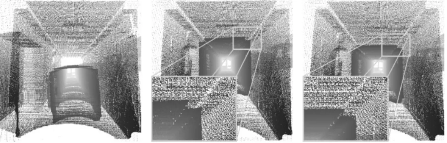
We calculate the transformation共R,t兲that maps the last pose of such a trajectory patch to the starting pose of the next patch. This transformation is then used to correct the trajectory patch by distributing the transformation as described in Section 3.4. In this way the algorithm computes a continuous trajectory. Figure 11. Scan matching of the IAIS robotic lab. Left: initial pose of two 3D scans. Middle: pose after five ICP iterations. Right: final alignment.

Figure 12. Left: initial poses of 3D scans when closing the loop. Middle: poses after detecting the loop and equally sharing the resulting error. Right: final alignment after error diffusion with correct alignment of the edge structure at the ceiling.

An animation of the scanned area is available at http://kos.informatik.uni-osnabrueck.de/

download/6Doutdoor/. The video shows the scene along the trajectory as viewed from about 1 m above Kurt3D’s actual position.

The 3D scans were acquired within one hour by tele-operation of Kurt3D. Scan registration and closed loop detection took only about ten minutes on a Pentium-IV-2800 MHz, while we did run the global relaxation for two hours. However, comput-ing the flight-thru-animation took about three hours, rendering 9882 frames with OpenGL on consumer hardware.

5.5. Stress Tests—RoboCup Rescue

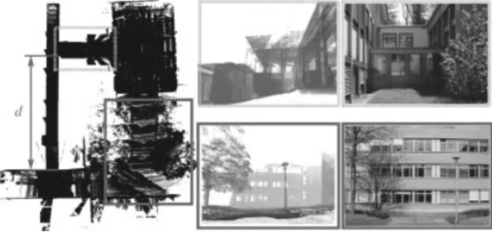
Our 3D mapping algorithms have been tested in various experiments. We participate in RoboCup Rescue competitions on a regular basis. RoboCup is an international joint project to promote AI, robotics, Figure 13. The closed loop with a top viewing position

and orthogonal projection. The distancedmeasured in the point cloud model is 2096 cm, measured by meter rule 2080 cm. The right part demonstrates the change in eleva-tion. Top right: a ramp connecting two buildings is cor-rectly modeled共height difference 1.05 m兲. The ramp con-nects the basement of the left building with the right building. Bottom right: outdoor environment modeling of the downhill part.

Figure 14. Three-dimensional model of an experiment to digitize part of the campus of Schloss Birlinghoven campus

共top view兲. Left: registration based on odometry only. Right: model based on incremental matching right before closing the loop, containing 62 scans each with approx. 100 000 3D points. The grid at the bottom denotes an area of 20

and related fields. It is an attempt to foster AI and intelligent robotics research by providing standard problems where a wide range of technologies can be integrated and examined. Besides the well-known RoboCup soccer leagues, the Rescue league is get-ting increasing attention. Its real-life background is the idea of developing mobile robots that are able to operate in earthquake, fire, explosive and chemical disaster areas, helping human rescue workers to do

their jobs. A fundamental task for rescue robots is to find and report injured persons. To this end, they need to explore and map the disaster site and in-spect potential victims and suspicious objects. The RoboCup Rescue Contest aims at evaluating rescue robot technology to speed up the development of working rescue and exploration systems 共NIST, 2007兲.

These kinds of competitions allow us to measure Figure 15. Top left: model with loop closing, but without global relaxation. Differences to Figure 14 right and to the right image are marked. Top right: final model of 77 scans with loop closing and global relaxation. Bottom: aerial view of the scene. The points A–D are used as reference points in the comparison in Table II.

the level of system integration and the engineering skills of the teams to be evaluated. It makes high demands on the reliability of the algorithms, since one cannot redo the experiments. A total of 21 robot runs were performed by Kurt3D in the World

Cham-pionships over the last three years. One major sub-goal of such a rescue mission is to create a map of the unstructured environment during the mission time. The test field is a square with six meter-long sides. Detailed maps of the environment have been Figure 16. Closeup view of the 3D model of Figure 15. Left: model before loop closing. Right: after loop closing, global relaxation and adding further 3D scans. Top: top view. Bottom: front view.

presented to the referees. Figure 19 shows one such map. With the superimposed grid in Figure 19 the referees evaluated the maps facilely.

In addition to the RoboCup Rescue competi-tions, the proposed algorithms have also been tested at the European Land Robotics Trial, ELROB

共FGAN, 2007兲. Please refer to http://

kos.informatik.uni-osnabrueck.de/download/ LisbonគRR/ and http://kos.informatik.uni-osnabrueck.de/download/elrob2006/ for some results.

5.6. Benchmarking Mapping Results

Bechmarking experiments are used for measuring the objective performance of a dedicated algorithm. In the past, many researchers published their results in the Radish共The Robotics Data Set Repository兲 re-pository 共Howard and Roy, 2006兲. These data sets are accompanied by maps depicted as figures. Most

researchers aimed at creating consistent maps. Re-cently, on the theoretical side of SLAM, Bailey, Nieto, Guivant, Stevens & Nebot, 共2006a兲proves that EKF-SLAM fails in large environments and FastEKF-SLAM is inconsistent as a statistical filter: It always underes-timates its own error in the medium to long-term 共Bailey, Nieto & Nebot, 2006b兲. Besides focusing on these consistency issues, little effort at correctness has been made in the SLAM community.

Testing algorithms and heuristics for objective correctness includes providing ground truth data. In computer vision research, it is a common technique to provide hand-labeled ground truth images and algorithms that calculate performance metrics. Up to now, such a performance metric is missing for SLAM algorithms. In this paper, we choose a sketchy comparison with uncalibrated aerial images. In on-going work, we provide a novel method for evalu-ating SLAM algorithms applied to large-scale prob-lems based on given ground truth maps and a Monte Carlo localization in these maps 共Wulf, Nüchter, Hertzberg & Wagner, 2007兲. A valuable source for state of the art performance are competi-tions 共cf., Section 5.5兲that, however, aim to evaluate whole systems under operational conditions and are not well suited for measuring the performance of one single algorithm.

6.

CONCLUSIONS AND FUTURE WORK

This paper has presented a new solution to the simul-taneous localization and mapping 共SLAM兲 problem Table II. Length ratio comparison of measured distances

in the aerial photographs with distances in the point model as shown in Figure 15.

1st line 2nd line

Ratio in aerial views

Ratio in

point model Deviation

AB BC 0.683 0.662 3.1%

AB BD 0.645 0.670 3.8%

AC CD 1.131 1.141 0.9%

CD BD 1.088 1.082 0.5%

with six degrees of freedom. The method is based on ICP scan matching, with odometry extrapolation, ini-tial pose estimation using a coarse-to-fine strategy with an octree representation, and closing loop detec-tion. Furthermore, the paper investigates approxi-mate data association usingkd-trees and a novel ex-act data association called cachedkd-tree search.

We see a number of basically independent ideas work together in our 6D SLAM approach. ICP is now

among the standard algorithms for scan registration; our contribution with respect to using it is to make it efficient for 6D registration of 3D scans by using oc-tree representation, point reduction andkd-trees, in-cluding approximation and caching.

Next, having ICP available in an on-line on-board version for 6D registration of 3D scans allows 6D scan registration to be used as a means for posterior pose correction, based on the rich amount of pose differ-ence information that 3D scans yield. As a conse-quence, we can afford to use just one pose rather than a distribution of poses as in probabilistic approaches: our pose tracking, aided by 6D scan registration共i.e., the prior pose estimation as modified by the posterior correction gained from registration兲, is typically suf-ficiently accurate.

Third, loop closing is another common topic in SLAM; here we profit again from the relatively accu-rate and robust posterior 6D pose estimation.

A rich set of experiments, including competi-tions, has confirmed our approach. In fact, more ex-periment data sets than those presented previously, have been used and are available共see below兲.

The algorithms are implemented without using probabilistic concepts. Keeping track of multi-hypotheses leads to enormous computational re-quirements which cannot currently be made available on a mobile platform. This dependence on one hy-pothesis has led us to methods that improve incre-Figure 18. The trajectory after mapping shows gaps,

since the robot poses are corrected at 3D scan poses.

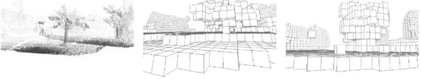
Figure 19. Three-dimensional maps of the yellow RoboCup arena. The 3D scans include spectators that are marked with a rectangle. Left: mapped area as 3D point cloud. Middle: voxel 共volume pixel兲 representation of the 3D map. Right: mapped area共top view兲. The points on the ground have been colored in light gray. The 3D scan positions are marked with squares. A 1 m2_{grid is superimposed. Following the ICP scan matching procedure, the first 3D scan defines the} coordi-nate system and the grid is rotated.

mentally the 6D pose estimate. However, in future work, we plan to adapt concepts from probabilistic robotics, like explicit representations of uncertainties, i.e., computing covariance matrices from scan match-ing. Furthermore, we will focus on multi-robot 3D mapping and on integrating vision sensors in the mapping system.

To foster research in Quantitative Performance Evaluation of Robotic and Intelligent Systems we will continue participating in the NIST evaluation, e.g., at RoboCup Rescue events. In addition, we plan to start a public 3D scan repository, to make 3D scans avail-able to the robotics community, like the Radish共The Robotics Data Set Repository兲 repository 共Howard and Roy, 2006兲. Material can currently be accessed under http://kos.informatik.uni-osnabrueck.de/ 3Dscans/.

REFERENCES

Allen, P., Stamos, I., Gueorguiev, A., Gold, E., & Blaer, P.

共2001兲. AVENUE: Automated Site Modelling in Urban Environments. In Proceedings of the Third Interna-tional Conference on 3D Digital Imaging and Model-ing共3DIM ’01兲, Quebec City, Canada.

Arun, K. S., Huang, T. S., & Blostein, S. D. 共1987兲. Least square fitting of two 3-d point sets. IEEE Transactions on Pattern Analysis and Machine Intelligence, 9共5兲, 698–700.

Arya, S. & Mount, D. M. 共1993兲. Approximate nearest neighbor queries in fixed dimensions. In Proceedings of the 4th ACM-SIAM Symposium on Discrete Algo-rithms, pages 271–280.

Arya, S., Mount, D. M., Netanyahu, N. S., Silverman, R., & Wu, A. Y.共1998兲. An Optimal Algorithms for Approxi-mate Nearest Neighbor Searching in Fixed Dimen-sions. Journal of the ACM, 45, 891–923.

Bailey, T., Nieto, J., Guivant, J., Stevens, M., & Nebot, E.

共2006a兲. Consistency of the EKF-SLAM Algorithm. In Proceedings of the IEEE/RSJ International Conference on Intelligent Robots and Systems共IROS ’06兲, Bejing, China.

Bailey, T., Nieto, J., & Nebot, E.共2006b兲. Consistency of the FastSLAM Algorithm. In IEEE International Confer-ence on Robotics and Automation 共ICRA ’06兲, Or-lando, Florida, U.S.A..

Benjemaa, R. & Schmitt, F.共1997兲. Fast Global Registration of 3D Sampled Surfaces Using a Multi-Z-Buffer Tech-nique. In Proceedings IEEE International Conference on Recent Advances in 3D Digital Imaging and Mod-eling共3DIM ’97兲, Ottawa, Canada.

Bentley, J. L.共1975兲. Multidimensional binary search trees used for associative searching. Communications of the ACM, 18共9兲, 509–517.

Besl, P. & McKay, N.共1992兲. A method for Registration of

3-D Shapes. IEEE Transactions on Pattern Analysis and Machine Intelligence, 14共2兲, 239–256.

Biber, P., Andreasson, H., Duckett, T., & Schilling, A.

共2004兲. 3D Modeling of Indoor Environments by a Mobile Robot with a Laser Scanner and Panoramic Camera. In Proceedings of the IEEE/RSJ International Conference on Intelligent Robots and Systems共IROS ’04兲, Sendai, Japan.

Dissanayake, M. W. M. G., Newman, P., Clark, S., Durrant-Whyte, H. F., & Csorba, M. 共2001兲. A Solution to the Simultaneous Localization and Map Building共SLAM兲 Problem. IEEE Transactions on Robotics and Automa-tion, 17共3兲, 229–241.

Eggert, D., Fitzgibbon, A., & Fisher, R. 共1998兲. Simulta-neous Registration of Multiple Range Views Satisfy-ing Global Consistency Constraints for Use In Reverse Engineering. Computer Vision and Image Under-standing, 69, 253–272.

FGAN共2007兲. http://www.elrob2006.org/.

Folkesson, J. & Christensen, H. 共2003兲. Outdoor Explora-tion and SLAM using a Compressed Filter. In Pro-ceedings of the IEEE International Conference on Ro-botics and Automation 共ICRA ’03兲, pages 419–426, Taipei, Taiwan.

Frese, U. & Hirzinger, G.共2001兲. Simultaneous Localiza-tion and Mapping—A Discussion. In Proceedings of the IJCAI Workshop on Reasoning with Uncertainty in Robotics, pages 17–26, Seattle, USA.

Friedman, J. H., Bentley, J. L., & Finkel, R. A.共1977兲. An algorithm for finding best matches in logarithmic ex-pected time.. ACM Transaction on Mathematical Soft-ware, 3共3兲, 209–226.

Früh, C. & Zakhor, A.共2001兲. 3D Model Generation for Cities Using Aerial Photographs and Ground Level Laser Scans. In Proceedings of the Computer Vision and Pattern Recognition Conference 共CVPR ’01兲, Kauai, Hawaii, USA.

Georgiev, A. & Allen, P. K.共2004兲. Localization Methods for a Mobile Robot in Urban Environments. IEEE Transaction on Robotics and Automation共TRO兲, 20共5兲, 851–864.

Greenspan, M. & Yurick, M.共2003兲. Approximate K-D Tree Search for Efficient ICP. In Proceedings of the 4th IEEE International Conference on Recent Advances in 3D Digital Imaging and Modeling 共3DIM ’03兲, pages 442–448, Banff, Canada.

Hebert, M., Deans, M., Huber, D., Nabbe, B., & Vandapel, N.共2001兲. Progress in 3-D Mapping and Localization. In Proceedings of the 9th International Symposium on Intelligent Robotic Systems, 共SIRS ’01兲, Toulouse, France.

Howard, A. & Roy, N.共2003–2006兲. Radish: The Robotics Data Set Repository, Standard data sets for the robot-ics community. http://radish.sourceforge.net/ Kohlhepp, P., Walther, M., & Steinhaus, P.共2003兲.

Schrit-thaltende 3D-Kartierung und Lokalisierung für mo-bile Inspektionsroboter. In Dillmann, R., Wörn, H., & Gockel, T., editors, Proceedings of the Autonome Mo-bile Systeme 2003, 18. Fachgesprche.

Leonard, J. J. & Durrant-Whyte, H. F.共1991兲. Mobile robot localization by tracking geometric beacons. IEEE