Investigating the Balassa-Samuelson hypothesis in transition: Do we understand what we see?

(1)

BOFIT

Discussion Papers

Balázs Égert

Investigating the Balassa-Samuelson

hypothesis in transition:

Do we understand what we see?

2002 • No. 6

Bank of Finland

Institute for Economies in Transition

, BOFIT

(2)

Ms Tarja Kauppila, economist Polish economy

Issues related to the EU enlargement [email protected]

Ms Tuuli Koivu, economist Baltic economies

[email protected]

Mr Tuomas Komulainen, economist Russian financial system

Currency crises

[email protected]

Mr Iikka Korhonen, research supervisor Baltic economies

Issues related to the EU enlargement [email protected]

Mr Timo Harell, editor Press monitoring [email protected]

Ms Liisa Mannila, department secretary Department coordinator

Publications traffic [email protected]

Ms Päivi Määttä, information specialist Institute’s library

Information services [email protected]

Ms Tiina Saajasto, information specialist Statistical analysis

statistical data bases Internet sites

[email protected]

Ms Liisa Sipola, information specialist Information retrieval

Institute’s library and publications [email protected]

Mr Vesa Korhonen, economist Russian economy and economic policy [email protected]

Mr Juhani Laurila, senior adviser Russian economy and economic policy Baltic countries’ external relations [email protected]

Mr Jouko Rautava, economist Russian economy and economic policy [email protected]

Mr Jian-Guang Shen, economist Chinese economy

[email protected] Ms Laura Solanko, economist Federarlism

Russian regional issues

Ms Merja Tekoniemi, economist Russian economy and economic policy [email protected]

Economists

Information Services

Mr Pekka Sutela, head

Russian economy and economic policy Russia’s international economic relations Baltic economies

[email protected]

Bank of Finland

Institute for Economies inTransition, BOFIT PO Box 160 FIN-00101 Helsinki

Contact us

Phone: +358 9 183 2268 Fax: +358 9 183 2294 E-mail: [email protected]

(3)

BOFIT

Discussion Papers

Balázs Égert

Investigating the Balassa-Samuelson

hypothesis in transition:

Do we understand what we see?

2002 • No. 6

Bank of Finland

Institute for Economies in Transition

, BOFIT

(4)

BOFIT Discussion Papers 6/2002

Balázs Égert :

Investigating the Balassa-Samuelson

hypothesis in transition: Do we understand what we see?

ISBN 951-686-828-2 (print) ISSN 1456-4564 (print) ISBN 951-686-829-0 (online) ISSN 1456-5889 (online)

(5)

Balázs Égert

1

Investigating the Balassa-Samuelson hypothesis

in transition: Do we understand what we see?

Abstract

This paper studies the Balassa-Samuelson effect in the Czech Republic, Hungary, Poland, Slovakia and Slovenia. Time series and panel cointegration techniques are used to show that the BS effect works reasonably well in these transition economies during the period 1991:Q1 to 2001:Q2. However, productivity growth does not fully translate into price in-creases due to the structure of CPI indexes. We thus argue that productivity growth will not hinder the ability of the five EU accession candidates to meet the Maastricht criterion on inflation in the medium term. Moreover, the observed appreciation of the CPI-deflated real exchange rate is found to be systematically higher compared to the real appreciation justi-fied by the Balassa-Samuelson effect, particularly in the cases of the Czech Republic and Slovakia. This may be partly explained by the trend appreciation of the tradable-goods-price-based real exchange rate, increases in non-tradable sector prices due to price liberali-sation and demand-side pressures, and the evolution of the nominal exchange rate due to the exchange rate regime and magnitude of capital inflows.

-(/: E31, F31, O11, P17

.H\ZRUGV: Balassa-Samuelson effect, Productivity, Real Exchange Rate, Transition, Panel Cointegration

Forthcoming in The Economics of Transition, 2002, Vol. 10, No. 2, Summer

1_{PhD student, MODEM, University of Paris 10, 200, avenue de la République, 92001-Nanterre, France, Tel:}

++33 1 40 97 59 75, Fax: ++33 1 40 97 77 84, E-mail: [email protected]

I would like to thank Wendy Carlin, Przemek Kowalski and Kirsten Lommatzsch for their numerous valuable comments and suggestions on an earlier draft of this paper, as well as Peter Pedroni for technical help on panel cointegration, and Greg Moore for help in language editing.

(8)

Balázs Égert

Investigating the Balassa-Samuelson hypothesis

in transition: Do we understand what we see?

Tiivistelmä

Tutkimus käsittelee Balassa-Samuelsonin efektiä (BSE) Tšekin tasavallassa, Unkarissa, Puolassa, Slovakiassa ja Sloveniassa. Aikasarja- ja paneeliyhteisintegroituvuusmetodit osoittavat, että BSE oli olemassa näissä siirtymätalouksissa 1990-luvulla. On kuitenkin huomattava, että tuottavuuden muutos ei täysin näy hintojen nousussa kuluttajahintaindek-sin rakenteen takia. Tuottavuuden kasvu ei siten estä EU-jäsenyyttä hakeneita maita saa-vuttamasta Maastrichtin inflaatiokriteeriä. Valuuttakurssin havaittu reaalinen vahvistumi-nen on suurempaa kuin BSE yksin antaisi odottaa. Tämä saattaa johtua esim. nimellisen valuuttakurssin vahvistumisesta, joka puolestaan saattaa aiheutua suurista pääomavirroista. Asiasanat: Balassa-Samuelsonin efekti, tuottavuus, reaalinen valuuttakurssi, transitio,

(9)

1 Introduction

Since beginning of the transformation process from centrally planned to market economies, Central Europe’s transition countries have experienced relatively high inflation and marked real appreciation of their currencies. It has become something of a stylised fact coming under the heading of the Balassa-Samuelson hypothesis that these phenomena are in part a consequence of strong productivity growth in the traded sector. The occurrence of such price increases naturally has repercussions for monetary policy. As EU accession candi-dates need to achieve nominal convergence as defined in the Maastricht criteria, inflation differentials stemming from productivity growth differentials have potential political con-sequences.

The Balassa-Samuelson effect in the transition countries has been examined in nu-merous studies.1 As the sample data are limited to just over a decade of transition and as most useful time series are available only on an annual basis, studies typically use panel estimations for a large number of transition countries. Thus, a great degree of homogeneity across countries, ranging from the most advanced Central European countries to the CIS, had to be assumed in the investigations.

Here, we examine the empirical validity of the Balassa-Samuelson hypothesis using quarterly data for five advanced Central European countries: the Czech Republic, Hungary, Poland, Slovakia and Slovenia. Employing both time series and panel cointegration tech-niques, we allow for a high degree of heterogeneity across countries. In addition, we quan-tify the impact of the productivity growth differential on overall inflation and investigate the extent to which this accounts for the real appreciation of the exchange rate in each country. Although we establish the Balassa-Samuelson effect in every country, its impor-tance is found to differ substantially. As regards EU accession and EMU run-up phase, we conclude that, despite marked productivity gains (especially in Hungary and Poland), the inflation differential associated with the Balassa-Samuelson effect is less of an issue than suggested in earlier research. Instead, we argue that stabilising the nominal exchange rate may be a more challenging task given liberalised capital accounts and large capital inflows. In the next section, we present a brief exposition of the Balassa-Samuelson model. Section III describes our data set in detail and provides a preliminary data analysis. Section IV provides an overview of the time series and panel econometric techniques used in this paper. Section V presents the empirical results. In Section VI, we compute inflation rates and the real exchange rate appreciation consistent with the Balassa-Samuelson effect. Sec-tion VII discusses policy implicaSec-tions of our findings and SecSec-tion VIII concludes.

2 The model

The Balassa-Samuelson effect, often labelled as the productivity bias hypothesis, is based on the model of a small open economy with two sectors: a sector producing tradable goods and one producing non-tradable goods. The model rests on two assumptions. On one hand, capital is perfectly mobile both across countries and across the two sectors of the economy, which implies that the interest rate is set in world markets and thus exogenous. On the

1

Cf. e.g. Halpern-Wyplosz (1997), Halpern-Wyplosz (2001), Coricelli-Jazbec (2001) DeBroeck-Sløk (2001) and Golinelli-Orsi (2001).

(10)

other hand, while labour is internationally immobile, it is assumed to be perfectly mobile domestically between the open and sheltered sectors. Nominal wages are determined in the tradables sector and, due to the wage equalisation process, hold for the entire economy.

The supply side of the two sectors can be described with the aid of two different, con-stant returns to scale Cobb-Douglas production functions as:

YT = AT ·(LT) (KT) (1) YNT = ANT ·(LNT) (KNT) . (2)

In these equations, AT, ANT, LT, LNT, KT and KNT denote the level of total factor productiv-ity, labour and capital in the open and sheltered sectors, respectively. Profit maximisation implies that interest rates (i) and nominal wages (w) in both sectors equal the marginal products dYT/dKT, dYNT/dKNT, dYT/dLT and dYNT/dLNT , respectively, as shown in equa-tions (3)-(6) expressed in logarithmic terms2.

iT ORJ DT NT – lT) (3)

iNT = (pNT - pTORJ DNT NNT – lNT) (4)

wT ORJ DT NT – lT) (5)

wNT = (pNT - pTORJ DNT NNT – lNT), (6)

where pNT and pT stand for prices of non-tradables and tradables. Perfect competition in the traded sector means that the prices of traded goods are exogenous. First-order conditions (FOC) in the tradables sector determine the capital-labour ratio, as capital is assumed to be fixed in the short term, and the nominal wage. Due to the wage equalisation process in the economy, the wage level is exogenous for the tradables sector. The FOC of the non-tradables sector thus determine the capital-labour ratio in the non-non-tradables sector and the relative price of non-tradables. For this model, then, the relative price of non-tradables and tradables is fully determined by the supply side conditions. To establish the connection between changes in the relative price of non-tradables compared to that of tradables (rela-tive prices) and the growth rate of productivity in the tradable sector rela(rela-tive to that in the non-tradable sector (dual productivity), equations (3) – (6) are totally differentiated and rearranged, leading to equation (7)3

(

NT T

)

( )

T NT

aˆ aˆ pˆ

pˆ − = δ γ ⋅ − , (7)

where circumflexes (ˆ) denote growth rates. Extending the model to a two-country frame-work and applying similar reasoning to the foreign country, equation (8) shows that the

2_{Lower case letters denote logarithms.}

(11)

difference between relative prices at home and abroad (relative price differential) is deter-mined by the difference between dual productivity at home and abroad (dual productivity differential).4

(

pˆNT −pˆT

) (

− pˆNT*−pˆT*

)

=

(

( )

δ γ ⋅aˆT −aˆNT

)

−

(

δ* γ*

)

⋅aˆT*−aˆNT*

)

(8)

To derive the relationship between the increase in the relative price of non-tradables and changes in the CPI deflated real exchange rate, we first decompose overall inflation into price increases for tradables and non-tradables in equation (9), where α and (1-α) stand for shares of the open and sheltered sectors of the economy. We then substitute this into the definition of the real exchange rate in equation (10). Substituting equation (9) into equation (10) yields equation (11):

(

)

NT T pˆ 1 pˆ pˆ=α⋅ + −α ⋅ (9) pˆ * pˆ eˆ rˆ= + − (10)

(

1

)

(

pˆ pˆ

)

(

1 *

)

(

pˆ * pˆ *

)

pˆ * pˆ eˆ rˆ= + T − T − −α NT − T + −α NT − T (11)

Real and nominal exchange rates are defined in domestic currency units per foreign cur-rency. An increase (decrease) in the exchange rate reflects depreciation (appreciation) of the domestic currency. Assuming that α equals α* and that relative PPP holds for tradable goods, equation (11) can be further simplified to

Uˆ=−

(

1−α

)

(

Sˆ17 −Sˆ7

) (

− Sˆ17 *−Sˆ7 *

)

. (12)

Combining equations (7) and (12) provides the direct link between the dual productivity differential and the CPI-based real exchange rate.

rˆ=−

(

1−α

)

(

δ γ⋅aˆT −aˆNT

) (

− δ* γ*⋅aˆT *−aˆNT *

)

(13)

Hence, to the extent that dual productivity at home exceeds that abroad, the domestic cur-rency will appreciate in real terms.

(12)

3 Description of the data

We consider the Czech Republic, Hungary, Poland, Slovakia and Slovenia, using quarterly labour productivity data, the relative price of non-tradables and real exchange rates. The sample period is 1991:Q1 to 2001:Q2. All data are seasonally adjusted and transformed by taking natural logarithms. Germany, the United States and a synthetic basket based on German and US data serve as the foreign country in this paper. Weights for the basket are derived from the currency settlement in foreign trade in 1999.5

Average labour productivity is used as a proxy for the marginal total factor productiv-ity suggested by the theoretical model. Productivproductiv-ity is computed as the index of industrial production divided by the index of employment in that sector. Industrial production and the employment series are issued from the monthly database of the WIIW on transition economies.6 As data at quarterly frequency are unavailable for labour productivity in the sheltered sector, we set it to zero. This seems a reasonable hypothesis as long as the non-tradable sector’s productivity gains remain approximately equal across countries. The rela-tive price of non-tradables is determined as changes in the price of services compared to the producer price index of final industrial goods. We assume services are the least likely to be traded, while industrial goods are likely to be traded and thus can be used as good proxies for non-tradable and tradables. The source of the price series is the OECD’s MEI7 and the WIIW monthly database. Nominal exchange rates are averages of average monthly rates vis-à-vis the German mark and the US dollar, and are obtained from the WIIW’s da-tabase. They are expressed as domestic currency units per one foreign currency unit.

We conduct single-equation Augmented Dickey-Fuller (ADF) and Phillips-Perron (PP) unit root tests both in levels and first differences to determine the order of integration of the series. Employing the standard testing strategy described in Bourbonnais-Terassa (1998), we first estimate the model including a trend and constant term, and then jointly test the null hypotheses of non-stationarity and the significance of the trend. If the tests reveal that the series is not trend-stationary, the model containing a constant is then esti-mated. When the series does not turn out to be stationary or non-stationary around a con-stant, the model without trend and constant is examined. The appropriate lag length is de-termined using the Schwarz information criterion. The results indicate that the variables are clearly I(1) processes. The exception is the Czech relative price of non-tradables com-pared to the US, as the PP test rejects the null of the unit root in level with a constant term.

4 Econometric techniques

Given the I(1) nature of the series, the cointegration analysis is employed to explore the long-run relationships developed in Section II. We then test the Balassa-Samuelson effect in two stages. In the first stage, we explore the internal transmission mechanism between dual productivity and relative prices according to equation (7). In the second stage, we in-vestigate the external transmission mechanism of the Balassa-Samuelson effect in a

5_{As regards Germany, the weights we use are 80%, 82%, 62%, 74% and 89% for the Czech Republic,}

Hungary, Poland, Slovakia and Slovenia, respectively. The weights for the US are 20%, 18%, 38%, 26% and 11%, respectively.

6_{Vienna Institute for International Economic Studies, www.wiiw.ac.at} 7_{Main Economic Indicators, www.sourceoecd.org}

(13)

country framework. We test to determine, in accordance with equation (8), if the dual pro-ductivity differential and the relative price differential are related. We also test to see if the relative price differential is linked to real exchange rate movements (equation 12). Finally, we examine whether changes in real exchange rates are driven exclusively by differences in relative price developments. The Balassa-Samuelson model rests on the assumption that the strong version of relative PPP holds for tradables, which implies stationarity of the PPI-deflated real exchange rate, so we also perform ADF and PP tests for stationarity of the PPI-based exchange rate.

The above cointegration relationships are investigated using two types of cointegra-tion techniques: the VAR-based multivariate cointegracointegra-tion methodology of Johansen (1988) developed for time series and the panel cointegration methodology proposed by Pedroni (1999, 2000).

For the time series cointegration analysis, we first specify a bivariate Vector Error Correction Model (VECM) for the internal transmission mechanism. We aim at establish-ing one cointegration relationship of the dual productivity and relative prices. Subse-quently, we proceed to testing of the external transmission mechanism. The latter is im-plemented by specifying a trivariate VECM including the dual productivity differential, the relative price differential and changes in the CPI-deflated real exchange rate. We seek to detect two long-term cointegrating vectors between the dual productivity differential and the relative price differential on the one hand, and between the relative price differential and changes in the CPI-deflated real exchange rate, on the other hand. 8 The presence of statistically significant cointegrating vectors in both cases would imply a long-run relation-ship between productivity and the CPI-based real exchange rate. This is the reason why we estimate this cointegration vector as well. If only one long-run relationship can be estab-lished, we go on to estimate a bivariate VECM for the relationship of the dual productivity differential and the relative price differential. In the case we are able to detect cointegra-tion, we found the long-term relationship. Otherwise, we specify another bivariate VECM for the relative price differential and changes in the real exchange rate so as to obtain the cointegrating vector detected in the three-variable VECM.

To obtain robust estimates of the cointegrating vectors, we implement a number of specification tests. The lag lengths are determined to ensure no auto-correlation and nor-mality for the residuals. Further, we implement likelihood ratio tests to determine the trend polynomial in the cointegrating vector.9 The cointegration rank is determined using the Johansen cointegration test.107KHVWDELOLW\RIWKHFRLQWHJUDWLRQUDQNDQGVSDFH DUHYHU i-fied in line with suggestions in Hansen-Johansen (1993). Roots of the model and the auto-correlation and normality of the residuals are examined using correlograms and performing the Jarque-Bera multivariate test on single-equation residuals and the residual vector.

8_{In this case, the rank of cointegration is equal to 2. It is worth noting that if the rank of cointegration (the}

number of cointegrating vectors) is equal to the number of variables (n), that is r=3 in this case, all variables are stationary with no exception. When r=3, a VAR in levels is appropriate for estimation, while with r=0 a VAR in first differences needs to be employed. In the latter case, no long-term relationship in levels can be established.

9_{We test for restrictions on deterministic trend coefficients. The following five models can be distinguished:}

model 1 (m1): the I(0) series have zero mean, the cointegrating vector does not have an intercept; model 2 (m2): the I(0) series have non-zero mean, the cointegrating vector contains an intercept; model 3 (m3): the I(0) series have linear trends, the cointegrating vector includes a constant; model 4 (m4): both the I(0) series and the cointegrating equation have a trend; model 5 (m5): I(0) series have a linear trend, and the I(1) component contains a quadratic trend.

10

Only the trace test statistics are reported since the lambda-max test does not fit into a coherent testing strategy as noted in Johansen (1992).

(14)

Before turning to the panel cointegration technique, we ascertain that variables are I(1). To do this, we apply the panel unit root test proposed by Im, Pesaran and Shin (1997). To test the null of a unit root, we rely on t-bar statistics using the mean of individual ADF statistics. The advantage of this test is that it allows for heterogeneity in the autoregressive coefficient across the countries of the panel. Consider the following equation assuming a trend and a constant term:

7 W 1 L W \ E \ \ LW L L LW Q W L W L W L = ⋅ + ⋅ − + + ⋅ + = = − = −

∑

µ γ ε (14)

Thus, the null of + π_L = for each i is tested against the alternative hypothesis of

1 1 L 1 L + π_L < = π_L = = _L+ .

As in the time series case, we start by investigating the internal transmission mechanism. While it is possible to test for the rank of cointegration in the time series context, the panel cointegration technique does not yet allow detecting the number of cointegrating vectors. For this reason, when investigating the Balassa-Samuelson effect in the two-country case, we have to proceed with pair-wise estimations between the dual productivity differential and the relative price differential and subsequently between the relative price differential and changes in the real exchange rate. If we find two cointegration relationships, we can establish the long-run relationship between the dual productivity differential and rate of growth of the real exchange rate as in the time series case.

Analogous to Engle and Granger, the Pedroni panel cointegration method tests the null of no cointegration against the alternative hypothesis of cointegration using the residu-als obtained from the cointegrating regression:

7 W 1 L W [ \_L_W =α_L +β_L⋅ _L_W +δ_L⋅ +ε_L_W = = . (15) Out of the seven panel cointegration statistics developed by Pedroni, we choose those that best account for heterogeneity.11 The group mean panel cointegration statistics test the null hypothesis of + π_L = against the alternative hypothesis of + π_L <L=1 ZKHUH i denotes the autoregressive coefficient of the residuals. Two of the tests are based

on the non-parametric PP rho-statistic and statistic, while the third is an ADF-based t-statistic. To determine the coefficient of the cointegration vector, the panel fully modified ordinary least squares (FMOLS) estimator of Pedroni (2000) is employed. The lag length is allowed to differ across countries and is determined using the Newey-West method.

5 Empirical results

Before turning to the empirical results, the crucial assumption of wage equalisation be-tween the tradable and non-tradable sectors needs to be verified. With regard to the dy-namics of wage developments, relative wages (wNT- wT) should be mean reverting, which implies that even if there is a gap in levels between nominal wages across sectors, this gap would be stable over time. We therefore checked to see if nominal wage increases in the

11

The employed statistics permit heterogeneity in the slope coefficients, the constant term and the trend, as well as allow for heterogeneous autoregressive coefficient in the residuals.

(15)

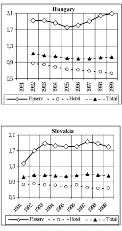
Figure 1. Relative wage developments, 1991-1999

6RXUFH: Countries in Transition 2000, WIIW Handbook of Statistics

1RWH “Finserv,” “Hotel” and “Total” refer to the following ratios: nominal wages in financial serv-ices/nominal wages in industry, nominal wages in the hotel industry/nominal wages in industry and the aver-age nominal waver-age of the economy/nominal waver-ages in industry.

&]HFK5HSXEOLF 0,5 0,9 1,3 1,7 2,1 19 91 19 92 19 93 19 94 19 95 19 96 19 97 19 98 19 99

Finserv Hotel Total

+XQJDU\ 0,5 0,9 1,3 1,7 2,1 19 91 19 92 19 93 19 94 19 95 19 96 19 97 19 98 19 99

Finserv Hotel Total

6ORYDNLD 0,5 0,9 1,3 1,7 2,1 1991 1992 1993 1994 1995 1996 1997 1998 1999

Finserv Hotel Total

6ORYHQLD 0,5 0,9 1,3 1,7 2,1 1991 1992 1993 1994 1995 1996 1997 1998 1999

Finserv Hotel Total 3RODQG 0,5 0,9 1,3 1,7 2,1 1991 1992 1993 1994 1995 1996 1997 1998 1999

(16)

non-tradable sector are related to nominal wage developments in industry. Using annual data for sectoral nominal wages for the period of 1991 to 1999, we compare the evolution of average nominal wages in the economy as a whole with that of wages in industry.12 Moreover, to reveal the dynamics on a more disaggregated level, we show the respective ratio for financial services and the hotel industry. In the case of Hungary and Poland (and possibly the Czech Republic), we encountered minor problems with wage equalisation, especially where wages in financial services to wages in industry were considered. How-ever, based on the visual inspection of Figure 1, our conclusion is that, on the whole, the ratio between nominal wages in different sectors of the economy remains rather stable over time.

We now turn to the results of the cointegration tests reported in Tables 1−5 and 7. The cointegration relationships are summarised in four vectors X1, X2, X3 and X4, where X1=[relative prices, dual productivity], X2=[relative price differential, dual productivity differential], X3=[the CPI-deflated real exchange rate, the relative price differential] and X4=[changes in the CPI-deflated real exchange rate, dual productivity differential]. Theory suggests that dual productivity and the dual productivity differential should be positively correlated with relative prices and the relative price differential. At the same time, we ex-pect a rise (fall) in the relative price differential and in the dual productivity differential to bring about an appreciation (depreciation) of the CPI-based real exchange rate. Techni-cally, the estimated coefficients of X1 and X2 in the time-series cointegration analysis should bear a negative sign while the estimates of β1 for X3 and X4 should be positively

signed. Concerning panel cointegration, the estimate of β1 of the X1 and X2 vectors should

enter with a positive sign. At the same time, the β1 of X3 and X4 should be negative.

Table 1 contains summary statistics for the Czech Republic. The cointegration tests reject the null of no cointegration for the internal linkage between dual productivity and relative prices. As can be seen from Table 1, the estimate of the coefficient is significant and has the correct sign. The stability tests also reveal that this relationship is stable over WLPHDVLVVSDFH +RZHYHUWKHFRHIILFLHQWLVORZHUWKDQRQHLQGLFDWLQJWKDWSURGXFWLYLW\ increases do not fully translate into increases in the relative price of non-tradables. Fur-thermore, we can establish statistically significant and correctly signed long-run relation-ships for the vectors X2, X3 and X4 when Germany and the trade-weighted basket are used as the benchmark. The estimated models are robust in terms of autocorrelation and nor-PDOLW\+RZHYHUZKLOHVSDFH VHHPVWREHVWDEOHZRUULHVDERXWWKHVWDELOLW\RIWKHFRL n-tegration rank equal to 2 arise, especially in the case of the basket, where the coinn-tegration rank becomes equal to 2 just at the very end of the period, casting doubt on the long-term connection between the relative price differential and the real exchange rate. The estimated coefficients suggest that increases in the relative price differential (X3) and the dual pro-ductivity differential (X4) are connected with a more than proportional appreciation of the real exchange rate. The results for the US as the foreign country clearly show that, even if we can find a long-run relationship between the dual productivity differential and the rela-tive price differential, the tests fail to reject the null of one cointegration relationship against the alternative hypothesis of two cointegrating vectors. In addition, while the coef-ILFLHQW 1 is significant and has the appropriate sign, the X2 vector is found rather unstable

during the period studied and the size of the estimated coefficient varies between models.13

12

The industrial sector includes manufacturing, mining and electricity.

13

(17)

Table 1. Johansen cointegration tests, Czech Republic

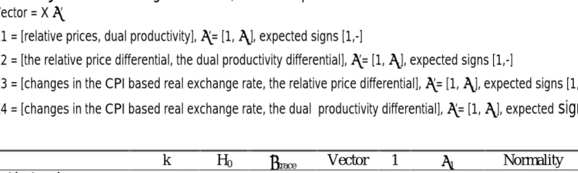
Vector = X β’

X1 = [relative prices, dual productivity], β’= [1, β1], expected signs [1,-]

X2 = [the relative price differential, the dual productivity differential], β’= [1, β1], expected signs [1,-]

X3 = [changes in the CPI based real exchange rate, the relative price differential], β’= [1, β1], expected signs [1,+] X4 = [changes in the CPI based real exchange rate, the dual productivity differential], β’= [1, β1], expected signs [1,+]

k H0 λtrace Vector 1 β1 Normality

&]HFK5HSXEOLF

K=2, m3 R=0 24.32** X1 1* -0.643 4.427 (0.351)

R=1 2.98 (-8.139)

*HUPDQ\

Prod, RPrice, RER K=1, m3 R=0 41.53** X2 1* -1.185 2.037 (0.916) R=1 14.82* (-5.085) R=2 1.53 X3 1* 1.441 (25.732) Prod, RER K=1, m3 R=0 18.57** X4 1* 1.884 1.275 (0.866) R=1 0.53 (5.037) %DVNHW

Prod, Rprice, RER K=1, m3 R=0 40.48** X2 1* -1.007 2.655 (0.851) R=1 16.25** (-5.009) R=2 2.37 X3 1* 1.311 (24.736) Prod, RER K=1, m3 R=0 21.00** X3 1* 1.473 2.488 (0.647) R=1 1.45 (4.829) 86

Prod, RPrice, RER K=1, m3 R=0 29.98** X2 1* -0.753 4.672 (0.587)

R=1 9.33 (2.768)

R=2 1.31 2

Prod, Rprice K=1, m4 R=0 28.89** X2 1 -0.342 4.320 (0.364)

R=1 5.14 (2.408)

1RWHλtrace is the Johansen statistics, critical values are those tabulated in Johansen(1996); * and ** indicate

that H0 is rejected at the 5% and 1% significance level, respectively;. the model tested for and the number of

lags used in the model are in parenthesis below the Johansen statistics. Below β1 values can be found the

t-statistics of the CE in parenthesis. The asterisk above the 1 in column 5, (the beta to which the cointegrating vector is normalised) indicates that the variable is significant at the 5% level in another normalisation. As UHJDUGVWKH-DUTXH%HUDQRUPDOLW\WHVWSYDOXHVDUHLQSDUHQWKHVLVEHQHDWK 2_{statistics and refer to skewness}

and kurtosis: normality is accepted when the p-value is higher than 0.05. When we could establish one coin-tegration relationship, only the corresponding cointegrating vector is reported (e.g. X2, while X3and X4 are not displayed in the table). RPrice and RER stand for the relative price differential and changes in the CPI-deflated real exchange rate, respectively.

(18)

The Johansen test (Table 2) detects the presence of a cointegrating vector between the Hungarian dual productivity and Hungarian relative prices. This estimate, which is signifi-cant at the 5% level and has the correct negative sign, strongly corroborates the prediction of the theoretical model. The specification tests reveal the robustness of the model, as there is no problem in terms of auto-correlation, normality, stability of the cointegration rank or VSDFH ,QWKHWZRFRXQWU\IUDPHZRUN7DEOHVKRZVWKDWDORQJUXQUHODWLRQVKLSFDQEH established between the dual productivity differential and the relative price differential no matter what benchmark country is chosen. These results are also quite robust as they passed all specification tests. The coefficients of the X2 cointegration vectors are highly significant and enter with the appropriate negative sign. Again, we find that increases in the productivity in the traded sector do not fully translate into increases in the prices of +XQJDULDQQRQWUDGDEOHV7KHFRLQWHJUDWLRQUDQNDQGVSDFH DUHIRXQGWREHYHU\VWDEOHDV the residuals satisfy the assumption of no auto-correlation and normal distribution. Even if normality is rejected at the 5% level for the two-variable model containing the dual pro-ductivity differential and the relative price differential with Germany as the foreign coun-try, the cointegration vector is well specified in the three-variable VECM. We should em-phasise here that, no matter which benchmark is chosen, the CPI-deflated real exchange rate does not seem to be related to either the relative price differential or the dual produc-tivity differential.

Table 2. Johansen cointegration tests, Hungary

Vector = X β’

X3 = [changes in the CPI based real exchange rate, the relative price differential], β’= [1, β1], expected signs [1,+]

K H0 λtrace Vector 1 β1 Normality

+XQJDU\

k=1, m3 R=0 37.22** X1 1* -0.694 6.073 (0.194)

R=1 0.59 (-2.168)

*HUPDQ\

Prod, Rprice, RER k=1, m3 R=0 54.79** X2 1* -1.204 5.612 (0.468)

R=1 9.88 (-16.722)

R=2 0.58

Prod, Rprice k=1, m3 R=0 37.22** X2 1* -1.200 11.788 (0.019) R=1 0.59 (-16.438)

%DVNHW

Prod, Rprice, RER k=1, m3 R=0 52.66** X2 1* -1.181 6.258 (0.395) R=1 12.41 (-16.634)

R=2 0.40

86

Prod, Rprice, RER k=1, m3 R=0 45.66** X2 1* -1.057 6.383 (0.382)

R=1 9.15 (-2.890)

R=2 0.09

Prod, Rprice k=1, m3 R=0 29.34** X2 1* -1.109 6.572 (0.160)

R=1 0.11 (13.202)

(19)

Table 3 shows a broadly similar picture in the case of Poland. We detect the presence of a long-run cointegration relationship for the internal transmission mechanism between dual productivity and relative prices. The determined coefficients are the lowest for the internal relationship among the investigated countries. The test results also provide clear empirical evidence for the existence of statistically significant and correctly signed cointegration relationships between the dual productivity differential and the relative price differential, on one hand, and between the relative price differential and the real exchange rate, on the other, when Germany is chosen as the foreign country. As might be expected, the dual pro-ductivity differential is cointegrated with the real exchange rate, which is consistent with the Balassa-Samuelson model. We note that productivity gains are accompanied by a dis-proportionate change in the real exchange rate. Nevertheless, these results suggest that while the dual productivity differential and the relative price differential of non-tradables appear to be connected in the long run when we consider either the basket or the US as the benchmark, movements in the relative price differential do not seem to be related to changes in the real exchange rate. It should be noted here that the VECM models specified for Polish data are extremely robust for several reasons. Most importantly, for each cointe-gration vector, the estimate of the coefficient is found to be always correctly signed and the t-statistics are comfortably large. Moreover, the results of the specification tests attest to the absence of auto-correlation and indicate that normality is not violated. Finally, stability WHVWVSHUIRUPHGRQWKHFRLQWHJUDWLRQUDQNDQGWKHVSDFH FOHDUO\UHMHFWLQVWDELOLW\IRUHYHU\ cointegration relationship.

Table 3. Johansen cointegration tests, Poland

Vector = X β’

3RODQG

k=1, m3 R=0 83.73* X1 1* -0.488 3.095 (0.542) R=1 0.24 (-22.182)

*HUPDQ\

Prod, Rprice, RER k=1, m3 R=0 99.24** X2 1* -0.763 3.617 (0.728) R=1 23.99* (17.744) R=2 1.31 X3 1* 1.852 (21.046) Prod, RER k=1, m3 R=0 36.18** X4 1* 1.320 3.390 (0.495) R=1 3.71 (18.082) %DVNHW

R=2 0.00

86

R=2 0.05

(20)

As reported in Table 4, in terms of the number of the detected cointegration relationships, the time-series cointegration analysis for Slovakia yields similar results as for Hungary. The Johansen tests provide a clear rejection of the null of no cointegration at the 1% level for the internal relationship between dual productivity and relative prices. In addition, we establish long-run cointegrating relationships between the dual productivity differential and the relative price differential, irrespective of the benchmark country. The tests fail, however, to detect a long-term relationship between the relative price differential and the real exchange rate, vis-à-vis our three benchmarks. A quick glance at the results initially seems to suggest that the estimated coefficients of the X2 vectors are statistically signifi-cant at the 1% level and bear the correct negative sign, but Jarque-Bera normality tests reveal that normality is rejected for four out of seven models. Moreover, while auto-correlation is not present in the residuals, we are unable to find a lag length that ensured normal distribution for the error terms for the estimates against the basket, the US and for the internal relationship. We should also note that according to the stability tests, the coin-WHJUDWLRQUDQNVZHGHWHFWHGDQGVSDFH WXUQRXWWREHVWDEOHRYHUWLPHLQGHSHQGHQWRIWKH internal transmission mechanism.

Table 4. Johansen cointegration tests, Slovakia

Vector = X β’

X3 = [changes in the CPI based real exchange rate, the relative price differential], β’= [1, β1], expected signs [1,+]

6ORYDNLD

k=1, m3 R=0 24.34** X1 1* -0.614 23.602 (0.000) R=1 0.21 (-6.396)

*HUPDQ\

Prod, RPrice, RER k=1, m2 R=0 42.56** X2 1* -3.604 10.500 (0.105) R=1 8.12 (-5.112)

R=2 1.70

%DVNHW

R=2 1.91

86

R=2 1.27

(21)

In the case of Slovenia (Table 5), the cointegration tests produce a clear rejection of the null of no cointegration at the 5% level for Slovenian dual productivity and relative prices. Despite the significant, correctly signed coefficient of the productivity variable and evi-dence of the stability of the detected cointegration relationship, the violation of the nor-mality assumption deserves comment. The latter clearly affects the robustness of the es-tablished long-run relationship. The empirical evidence in favour of the Balassa-Samuelson effect is straightforward when Germany and the basket are taken as the bench-mark; it is less clear when the US is considered as the foreign country. The results summa-rised in Table 5 uncover the presence of the cointegrating vectors X2, X3 and X4 for Ger-many and the trade-weighted basket. All estimated coefficients are significant and appro-priately signed. The specification tests confirm the robustness of our estimates. Just as in the case of the four other transition countries, productivity and relative prices only seem to be related using US data, while tests fail to establish any meaningful linkage between rela-tive prices and the real exchange rate.

Table 5. Johansen cointegration tests, Slovenia

Vector = X β’

K H0 λtrace Vector 1 β1 Normality

6ORYHQLD

k=1 m3 R=0 27.28* X1 1* -0.948 55.925 (0.000) R=1 3.19 (-10.478)

*HUPDQ\

Prod, Rprice, RER k=1, m2 R=0 74.99** X2 1* -3.537 2.037 (0.916) R=1 27.92** (-10.685) R=2 5.25 X3 1* 0.537 (8.391) Prod, RER k=2, m2 R=0 22.59** X4 1* 1.686 3.354 (0.500) R=1 5.01 (6.744) %DVNHW

Prod, Rprice, RER k=1, m2 R=0 83.77** X2 1* -3.338 2.655 (0.851) R=1 30.91** (-11.837) R=2 4.91 X3 1* 0.431 (8.979) Prod, RER k=2, m2 R=0 26.92** X4 1* 1.105 2.980 (0.561) R=1 6.19 (6.538) 86

R=2 2.78

(22)

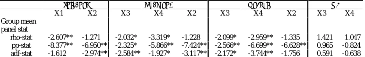
Finally, we construct a panel including the five transition economies for the period used in the time-series analysis. The motivation for using panel data is to increase the power of the cointegration tests. The first step in the analysis is to test for unit root. As the single ADF and PP tests previously indicated that 49 series out of 50 are I(1), it is not surprising that the Im-Pesaran-Shin panel unit root test assuming an intercept and trend and only a con-stant term seems to confirm that all series are I(1) processes. Table 6 gives the results of the Pedroni panel cointegration tests. We note all three types of group mean statistics, since they allow for maximum heterogeneity across countries and give no indication that the residuals’ autoregressive coefficient should be the same for all countries. Results in Table 6 indicate that the panel cointegration technique allows detection of more cointegration relationships than single-country analysis. Thus, we are now able to reject the null hy-pothesis of no cointegration against the alternative hyhy-pothesis of the existence of a cointe-grating relationship for the vectors X3 and X4 for all countries when Germany or the bas-ket serve as benchmark, i.e. also in the cases where time-series analysis could not detect such relationships (Poland vis-à-vis the basket and for Hungary and Slovakia vis-à-vis Germany and the basket). The panel cointegration analysis seems to confirm the results of the Johansen tests in cases where the US was used as a benchmark country: the relative price differential and the real exchange rate are not cointegrated for any countries.

Table 6. Panel Cointegration Statistics

,QWHUQDO *HUPDQ\ %DVNHW 86 X1 X2 X3 X4 X2 X3 X4 X2 X3 X4 Group mean panel stat rho-stat -2.607** -1.271 -2.032* -3.319* -1.228 -2.099* -2.959** -1.335 1.421 1.047 pp-stat -8.377** -6.950** -2.325* -5.866** -7.424** -2.566** -6.699** -6.628** 0.965 -0.824 adf-stat -1.612 -2.974** -2.584** -1.927* -3.117** -2.172* -3.744** -1.756 0.591 -0.638

Note: The Pedroni statistics (1999) are adjusted as proposed in Pedroni (2001). Critical values are based on the standard normal distribution; * and ** indicate that H0 is rejected at the 5% and 1% significance level,

respectively.

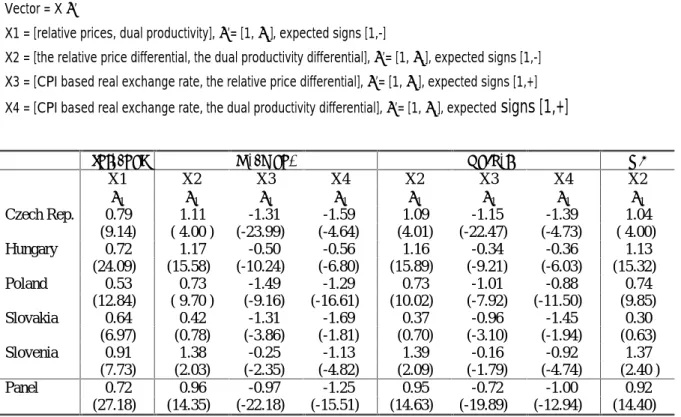
We use the panel FMOLS estimator to obtain the estimates for the coefficients of the cointegrating relationships we detected with the panel cointegration tests. As shown in Table 7, all coefficients are correctly signed.14 For the Czech Republic, Hungary and Po-land, each coefficient is similar to the value obtained from the time-series analysis and is significant at the 1% level. The case of Slovakia and Slovenia is somewhat puzzling in that the values of the coefficients are far lower than what we obtain from the Johansen tests. In DGGLWLRQQRQHRIWKHFRHIILFLHQWVIRU;LVVLJQLILFDQWIRU6ORYDNLDDQGWKHHVWLPDWHRI 1

for the X3 against the basket is not significant for Slovenia.

(23)

Table 7. Panel FMOLS estimates of the cointegrating vectors’ coefficients

Vector = X β’

X2 = [the relative price differential, the dual productivity differential], β’= [1, β1], expected signs [1,-] X3 = [CPI based real exchange rate, the relative price differential], β’= [1, β1], expected signs [1,+] X4 = [CPI based real exchange rate, the dual productivity differential], β’= [1, β1], expected signs [1,+]

,QWHUQDO *HUPDQ\ %DVNHW 86 X1 X2 X3 X4 X2 X3 X4 X2 β1 β1 β1 β1 β1 β1 β1 β1 Czech Rep. 0.79 1.11 -1.31 -1.59 1.09 -1.15 -1.39 1.04 (9.14) ( 4.00 ) (-23.99) (-4.64) (4.01) (-22.47) (-4.73) ( 4.00) Hungary 0.72 1.17 -0.50 -0.56 1.16 -0.34 -0.36 1.13 (24.09) (15.58) (-10.24) (-6.80) (15.89) (-9.21) (-6.03) (15.32) Poland 0.53 0.73 -1.49 -1.29 0.73 -1.01 -0.88 0.74 (12.84) ( 9.70 ) (-9.16) (-16.61) (10.02) (-7.92) (-11.50) (9.85) Slovakia 0.64 0.42 -1.31 -1.69 0.37 -0.96 -1.45 0.30 (6.97) (0.78) (-3.86) (-1.81) (0.70) (-3.10) (-1.94) (0.63) Slovenia 0.91 1.38 -0.25 -1.13 1.39 -0.16 -0.92 1.37 (7.73) (2.03) (-2.35) (-4.82) (2.09) (-1.79) (-4.74) (2.40 ) Panel 0.72 0.96 -0.97 -1.25 0.95 -0.72 -1.00 0.92 (27.18) (14.35) (-22.18) (-15.51) (14.63) (-19.89) (-12.94) (14.40) Note: t-values in parenthesis.

As mentioned above, the final step of our analysis is to test if the relative PPP holds for tradables and thus whether our results fully accord with the Balassa-Samuelson model. To this end, we conduct both single equation ADF and PP tests and the Im-Pesaran-Shin panel unit root test for the real exchange rate calculated using the industrial producer price index. Surprisingly, the null hypothesis of a unit root cannot be rejected at the conventional 5% level, irrespective of the type of the unit root test employed. The fact that the strong ver-sion of the relative PPP cannot be verified for tradable goods provides us with a valuable insight about real exchange rate behaviour − in addition to changes in relative prices play-ing a role in real exchange rate determination, movements in the prices of tradable goods also appear to influence the evolution of the CPI-based real exchange rate.

(24)

6 Quantifying the linkage of productivity growth,

inflation and appreciation of the real exchange rate

So far we have concentrated on the question of whether changes in productivity, relative prices and the real exchange rate are connected via a cointegrating vector. In the following section, we calculate the contribution of the Balassa-Samuelson effect to the inflation dif-ferential and the appreciation of the real exchange rate. In other words, our aim here is to quantify the impact of productivity gains on inflation and the real exchange rate.

We start by computing the inflation differential vis-à-vis Germany, assuming all five of these CEECs will eventually participate in the EMU. Meeting the Maastricht criterion on inflation implies that the inflation rate of an EMU aspirant will not exceed the average of the three lowest inflation rates of Euroland by more than 1.5% for at least one year be-fore entering EMU. In this regard, Germany makes a good proxy for the inflation criterion thanks to its impressive inflation track record. Applying the theoretical assumptions pre-sented in Section II, we derive the relationship between the dual productivity differential and the inflation differential between the home and the foreign country. Expressing the price of non-tradables in equation (7) and combining it with equation (9), we obtain the equation for overall inflation shown in equation (16):

(

)

(

T NT

)

T aˆ aˆ 1 pˆ pˆ= + −α δ γ⋅ − (16)

The inflation differential between countries is then related to the dual productivity differ-ential so that

(

1

) ( )

[

(

ˆ ˆ

)

(

* *

)

ˆ * ˆ *

)

]

* ˆ ˆ * ˆ ˆ S S7 S7 D7 D17 D7 D17 S− = − + −α δ γ ⋅ − − δ γ ⋅ − . (17) We next use equation (18) to determine the extent to which productivity is likely to affect the inflation differential15

(

1

)

[

(

aˆ aˆ

) (

aˆ * aˆ *

)

]

*

pˆ

pˆ− = −α β₁ T − NT − T − NT , (18)

ZKHUH 1 is the estimated coefficient of the X2 vector.

We use several methods to compute the inflation differential associated with the Ba-lassa-Samuelson effect. We consider the productivity data used in the estimations, as well as the trend obtained by employing the Hodrick-Prescott filter on the series.16 Next, the average yearly changes for three periods: the whole period and for two sub-periods,

15_{We set the tradable goods inflation differential to zero as we are interested in the inflation brought about by}

productivity gains. As equations (7) and (8) reveal, this inflation is always non-tradable inflation.

16_{The smoothing parameter is set equal to 1600 as proposed in Hodrick-Prescott (1997) for quarterly data.}

For a recent discussion on the appropriate value of the smoothing parameter for annual and quarterly data, see Ravn-Uhlig (2001).

(25)

tably for 1991:Q1 to 1995:Q4 and 1996:Q1 to 2001:Q2 are determined for the two types of series. We also determine the average annual change in productivity for each year.

6XEVWLWXWLQJWKHVHUHVXOWVLQWRHTXDWLRQZHILUVWRQO\FRQVLGHUWKH WHUP17

in the equation and ignore the estimates of the coefficient issued from the cointegrating vec-WRU:HWKHQHVWLPDWHWKHLQIODWLRQGLIIHUHQWLDOXVLQJERWK DQG 1. We use estimates of

1 coming both from the individual time-series analysis and the panel method.

Once we have quantified the inflation differential associated with the Balassa-Samuelson effect, we next attempt to determine how much real appreciation can be ex-plained by productivity gains. Here, we employ a slightly modified version of equation (13):

(

1

)

(

aˆ aˆ

) (

aˆ * aˆ *

)

rˆ=− −αβ₁ T − NT − T − NT . (19)

The procedure is similar to that described above with the difference that we use the esti-PDWHRI 1 of the cointegration vector X4. The real appreciation associated with the dual

productivity differential is then compared to the observed appreciation of the CPI-deflated real exchange rate. The results are reported in Tables 8, 9, 11 and 12.

Although results differ with regard to the countries and the time period studied (see Tables 8 and 9), the main features of the first results can be readily summarised. First, we observe sizeable productivity gains during the period studied − of the order of 2.7% to 3.6% for Hungary and 3.1% to 4.4% for Poland. Looking at the sub-periods suggests that the productivity growth relative to Germany has accelerated since the mid-1990, from 2.4% and 2.7% to as high as 5.5% and 5.8% for Hungary and Poland, respectively. As a result, in accordance with equation (18), the inflation differential vis-à-vis Germany due to the dual productivity differential amounts to between 2.2% and 3.1% for Hungary and 1.5% to 2.2% for Poland during the period 1991 to 2001. However, as productivity gains become greater over time, the inflation associated with the Balassa-Samuelson effect also rises to 4.3% or 4.6% in the case of Hungary, and 2.8% or 2.9% for Poland, depending on whether individual or panel estimates are used. Contrary to what we observe for the case of Hungary and Poland, the dual productivity differential compared to Germany is found to be slightly negative for Slovakia and Slovenia in the period 1991-2001. In the second half of that period, the dual productivity differential seems to accelerate in these countries tak-ing positive values, but still averages below 1% a year. Table 8 shows the striktak-ing negative effect of productivity on inflation for the entire period and in the first half of the 1990s. With higher productivity growth after 1996, the inflation differential also becomes positive and ranges between 0.02% and 1.9% for Slovakia and between 0.6% and 2.1% for Slove-nia. Note that the results differ substantially depending on whether panel or single-country estimates are used. On average, we can conclude that the dual-productivity-differential-driven inflation is rather modest in these two countries. The Czech Republic’s situation is somewhat different because its dual productivity differential has always exceeded Ger-many’s, although to a lesser extent than for Hungary or Poland. Hence, the impact of the

17_{7KH WHUPLVWKHVKDUHRIQRQWUDGDEOHJRRGVLQ*'3:HGHWHUPLQHLWDVWKHDQQXDODYHUDJHIRUWKH}

period of 1992 to 1998 using nominal sectoral GDP data obtained from the WIIW database on transition economies. The industrial sector is taken as the tradable goods sector, while the non-tradable goods sector includes the rest. We note that agriculture is not taken into account. So, the non-tradable goods share amounts to 61.6% for the Czech Republic, 70.1% for Hungary, 65.5% for Poland, 65.1% for Slovakia and 64.4% for Slovenia.

(26)

dual productivity differential on the inflation differential remains modest, ranging from 0.06% to 1.1%, depending on the period and the source of the coefficientestimates.

Table 8. The contribution of the Balassa-Samuelson effect to the inflation against Germany (with the share of non-tradables as in GDPa)

&]HFK

5HS +XQJDU\ 3RODQG 6ORYDNLD 6ORYHQLD 3DQHO 7KHGXDOSURGXFWLYLW\GLIIHUHQWLDODJDLQVW*HUPDQ\LQ Raw data 1991-2001 0.304 3.668 4.413 -0.696 -0.608 1.416 1991-1995 0.418 1.543 2.251 -1.523 -1.940 0.150 1996-2001 0.198 5.209 5.754 0.057 0.659 2.375 HP filter 1991-2001 0.083 2.730 3.082 -1.305 -0.450 0.828 1991-1995 1.445 2.423 2.771 -1.089 -0.504 1.009 1996-2001 1.229 5.484 5.815 0.805 0.904 2.847 7KHLQIODWLRQGLIIHUHQWLDOGXHWRWKH%DODVVD6DPXHOVRQHIIHFW XVLQJWKH WHUPLQHTXDWLRQ Raw data 1991-2001 0.187 2.571 2.890 -0.453 -0.391 0.967 1991-1995 0.257 1.082 1.474 -0.992 -1.249 0.112 1996-2001 0.122 3.651 3.769 0.037 0.424 1.607 HP filter 1991-2001 0.051 1.914 2.018 -0.850 -0.290 0.569 1991-1995 0.890 1.698 1.815 -0.709 -0.325 0.674 1996-2001 0.757 3.844 3.809 0.524 0.582 1.903 7KHLQIODWLRQGLIIHUHQWLDOGXHWRWKH%DODVVD6DPXHOVRQHIIHFW XVLQJWKH WHUPZKHUHEHWDVDUHHVWLPDWHVIURPWLPHVHULHVDQDO\VLV Raw data 1991-2001 0.222 3.096 2.205 -1.633 -1.384 1991-1995 0.305 1.303 1.125 -3.574 -4.419 1996-2001 0.144 4.396 2.875 0.133 1.501 HP filter 1991-2001 0.061 2.304 1.540 -3.063 -1.026 1991-1995 1.055 2.045 1.385 -2.555 -1.149 1996-2001 0.897 4.629 2.906 1.888 2.060 7KHLQIODWLRQGLIIHUHQWLDOGXHWRWKH%DODVVD6DPXHOVRQHIIHFW XVLQJWKH WHUPZKHUHEHWDVDUHHVWLPDWHVIURPSDQHOGDWD Raw data 1991-2001 0.206 3.009 2.110 -0.190 -0.540 0.888 1991-1995 0.283 1.266 1.076 -0.416 -1.724 0.094 1996-2001 0.134 4.272 2.751 0.016 0.586 1.490 HP filter 1991-2001 0.056 2.239 1.473 -0.357 -0.400 0.519 1991-1995 0.979 1.987 1.325 -0.298 -0.448 0.633 1996-2001 0.833 4.498 2.781 0.220 0.804 1.786 a_{7KH WHUPLVVHWHTXDOWRWKHVKDUHRIQRQWUDGDEOHVLQ*'3}

(27)

As far as the relationship between the dual productivity differential and the appreciation of the real exchange rate is concerned, the picture is broadly similar to what we obtain by analysing the extent to which the dual productivity differential may affect the overall con-sumer price index. In the case of Hungary and Poland, the national currency has experi-enced a real appreciation of 2.4%−3.2% and 4.3%−4.8%, respectively, for the whole pe-riod. As in the case of the dual productivity differential, real appreciation was higher in the second sub-period. Assessing the result obtained in accordance with equation (19), we ob-VHUYH WKDW ZLWK DQG ZLWKRXW 1, the observed real appreciation of the home currency is

strongly related to the Balassa-Samuelson effect. Of the countries examined, Slovenia’s currency had the lowest observed real appreciation − regardless of the period considered or the data used. This may be associated with the moderate fall in dual productivity during the period 1991−2001 and 1991−1995. The second sub-period provides evidence in favour of productivity-backed real appreciation, since the approximately 1.7% to 2.0% appreciation in real terms was accompanied by productivity gains exceeding German productivity growth by 0.6%−0.9%. Although Table 8 shows a large average yearly real appreciation of around 5% for both the Czech Republic and Slovakia, productivity progress remains quite low, and thus the associated real appreciation is also insignificant.18

Using weights based on national accounts as is usual practice, we assumed so far that the non-tradables’ share in the CPI basket is equal to that in the GDP deflator. The exami-nation of the officially published Czech and Hungarian consumer price basket reveals a strikingly different picture − non-tradables represent a mere 32.7% of the Czech basket between 1994 and 2000! Similarly, the average share of non-tradables was as low as 35% in Hungary over the period of 1993 to 2000, 33.9% for Slovakia for the period of 1997 to 1999 and 41% for Poland in 2000.19 Using these weights, we proceed to recalculate the contribution of the dual productivity differential to the inflation differential and the real appreciation of the home currency.

Tables 11 and 12 summarise the new results. The conclusion for the Czech Republic, Slovakia and Slovenia shows little change. The inflation differential vis-à-vis Germany due to the dual productivity differential remains quite low. More importantly, we see a dra-matic decrease in the inflation differential attributable to the Balassa-Samuelson effect for Hungary and Poland. Figures drop under the critical value of 1.5% in the periods 1991−1995 and 1991−2001. Examining the second period 1996−2001 yields figures for the inflation differential slightly above 1.5%.

18_{We also report results for the whole panel where possible. Although it is enticing to reason in terms of a}

panel of countries, we refrain for two reasons. First, in panel estimations, the same weight is attributed to every country. It is clear that Poland and Slovenia should not be treated with the same weights. Second, as the reported results make it clear, the countries are rather heterogeneous and therefore the same estimated coefficient should not be applied to all of them.

19

As we lack data on Slovenia, we assume the average weight of the other countries. Figures obtained from central bank statistics.

(28)

Table 9. The contribution of the Balassa-Samuelson effect to the appreciation of the real exchange rate against Germany (share of non-tradables in GDPa

) &]HFK

5HS +XQJDU\ 3RODQG 6ORYDNLD 6ORYHQLD 3DQHO 5HDODSSUHFLDWLRQMXVWLILHGE\WKH%DODVVD6DPXHOVRQHIIHFW XVLQJRQO\WKH WHUPLQHTXDWLRQ Raw data 1991-2001 0.187 2.571 2.890 -0.453 -0.391 0.967 1991-1995 0.257 1.082 1.474 -0.992 -1.249 0.112 1996-2001 0.122 3.651 3.769 0.037 0.424 1.607 HP filter 1991-2001 0.051 1.914 2.018 -0.850 -0.290 0.569 1991-1995 0.890 1.698 1.815 -0.709 -0.325 0.674 1996-2001 0.757 3.844 3.809 0.524 0.582 1.903 5HDODSSUHFLDWLRQMXVWLILHGE\WKH%DODVVD6DPXHOVRQHIIHFW XVLQJWKH WHUPZKHUHEHWDVDUHHVWLPDWHVIURPWLPHVHULHV Raw data 1991-2001 0.353 NA20 3.815 NA -0.660 1991-1995 0.485 NA 1.946 NA -2.107 1996-2001 0.229 NA 4.975 NA 0.715 HP 1991-2001 0.096 NA 2.664 NA -0.489 1991-1995 1.677 NA 2.396 NA -0.548 1996-2001 1.426 NA 5.028 NA 0.982 5HDODSSUHFLDWLRQMXVWLILHGE\WKH%DODVVD6DPXHOVRQHIIHFW XVLQJWKH WHUPZKHUHEHWDVDUHHVWLPDWHVIURPSDQHOGDWD Raw data 1991-2001 0.298 1.440 3.728 -0.766 -0.442 1.157 1991-1995 0.409 0.606 1.902 -1.676 -1.412 0.122 1996-2001 0.193 2.045 4.862 0.062 0.479 1.940 HP 1991-2001 0.081 1.072 2.604 -1.436 -0.328 0.676 1991-1995 1.415 0.951 2.342 -1.198 -0.367 0.824 1996-2001 1.204 2.153 4.913 0.885 0.658 2.326 2EVHUYHGDSSUHFLDWLRQRIWKH&3,EDVHGUHDOH[FKDQJHUDWH Raw data 1991-2001 4.611 2.436 4.267 4.109 0.500 3.185 1991-1995 5.908 0.643 3.306 4.873 -1.022 2.741 1996-2001 4.780 4.185 6.094 4.448 1.791 4.259 HP filter 1991-2001 4.892 3.153 4.868 4.495 1.552 3.792 1991-1995 6.172 1.617 3.475 4.998 -0.029 3.247 1996-2001 4.562 3.074 5.510 4.292 2.088 3.905 a_{7KH WHUPLVVHWHTXDOWRWKHVKDUHRIQRQWUDGDEOHVLQ*'3}

We also note that the share of regulated prices in the CPI remains high, even if it has gen-erally declined over the past decade. During the period 1991−1999, administered prices represented, on average, 15-20% of the CPI basket (see Table 10). Typically, administered prices apply extensively to services. At stake here is the transmission between productivity

20

Because of the missing cointegration vector, we could not compute the respective figures for Hungary and Slovenia.

(29)

growth and inflation. Consequently, the share of market-based services in the CPI, which provides the pass-through from productivity growth to overall inflation, is in fact lower that suggested above and may in fact drop below 30%. Hence, the figures presented in Ta-ble 11 and 12 should be revised downwards. The point here is that increases in adminis-tered prices likely exacerbate the increase in the relative price of non-tradables. Thus, there is a danger that the impact of non-tradables inflation on overall inflation may be wrongly interpreted as productivity growth.

Table 10. The share of administered prices in the CPI basket, 1991−1999 (%)

&]HFK5HSXEOLF 27.9 18.3 17.9 18.1 17.4 17.4 13.3 13.3 13.3 13.3

+XQJDU\ 11.0 10.9 10.8 11.8 12.9 12.8 15.9 n.a. n.a. n.a.

3RODQG 11.0 14.0 16.0 17.0 17.0 15.0 12.0 10.0 9.0 9.0

6ORYDNLD n.a. n.a. 21.8 21.8 21.8 21.8 15.1 14.7 15.2 n.a.

6ORYHQLD n.a. 23.7 19.8 18.4 22.5 22.4 20.4 17.0 14.3 13.7 Source: EBRD, Transition Report 2001

Based on Szapáry (2000), a growing body of literature calls for modifying the Maastricht inflation criterion since advanced transition countries will be unable to satisfy the criterion on price stability due to of the Balassa-Samuelson effect.21 Our results, conversely, provide hope that even Poland and Hungary will meet the Maastricht criterion on price stability because the structural inflation differential explained by the Balassa-Samuelson effect does not present an insurmountable obstacle for these two countries. Both can bring their infla-tion into line with the Maastricht criterion on price stability. That said, as these economies catch up in terms of per capita GDP, consumption is likely to shift towards non-tradables. This shift will be explicit when the composition of the CPI is modified to give more weight to non-tradable items. An automatic consequence of this change will be the increased im-pact of the dual productivity differential on the overall inflation differential vis-à-vis the rest of the world. Of course, playing catching-up in terms of productivity is a game with diminishing returns: the closer a country approaches the targeted EU average productivity level, the lower the dual productivity differential. Indeed, in the long term, lower dual pro-ductivity could counterbalance the evolution of CPI weights in favour of non-tradables.

(30)

Table 11. The inflation differential against Germany associated with the Balassa-Samuelson effect (share of non-tradables in CPIa

) &]HFK

5HS +XQJDU\ 3RODQG 6ORYDNLD 6ORYHQLD 3DQHO 7KHLQIODWLRQGLIIHUHQWLDOGXHWRWKH%DODVVD6DPXHOVRQHIIHFW XVLQJRQO\WKH WHUPLQHTXDWLRQ Raw data 1991-2001 0.100 1.284 1.809 -0.237 -0.213 0.549 1991-1995 0.137 0.540 0.923 -0.518 -0.679 0.081 1996-2001 0.065 1.823 2.359 0.019 0.231 0.899 HP filter 1991-2001 0.027 0.956 1.263 -0.444 -0.158 0.329 1991-1995 0.473 0.848 1.136 -0.370 -0.177 0.382 1996-2001 0.402 1.919 2.384 0.274 0.317 1.059 7KHLQIODWLRQGLIIHUHQWLDOGXHWRWKH%DODVVD6DPXHOVRQHIIHFW XVLQJWKH WHUPZKHUHEHWDVDUHHVWLPDWHVIURPWLPHVHULHVDQDO\VLV Raw data 1991-2001 0.118 1.546 1.380 -0.853 -0.752 1991-1995 0.162 0.650 0.704 -1.866 -2.402 1996-2001 0.077 2.195 1.800 0.070 0.816 HP filter 1991-2001 0.032 1.151 0.964 -1.600 -0.557 1991-1995 0.560 1.021 0.867 -1.335 -0.624 1996-2001 0.476 2.311 1.819 0.986 1.120 7KHLQIODWLRQGLIIHUHQWLDOGXHWRWKH%DODVVD6DPXHOVRQHIIHFW XVLQJWKH WHUPZKHUHEHWDVDUHHVWLPDWHVIURPSDQHOGDWD Raw data 1991-2001 0.109 1.502 1.321 -0.099 -0.293 0.483 1991-1995 0.150 0.632 0.674 -0.218 -0.937 0.051 1996-2001 0.071 2.133 1.722 0.008 0.318 0.810 HP filter 1991-2001 0.030 1.118 0.922 -0.186 -0.217 0.282 1991-1995 0.520 0.992 0.829 -0.156 -0.244 0.344 1996-2001 0.442 2.246 1.740 0.115 0.437 0.972 a_{7KH WHUPLVVHWHTXDOWRWKHVKDUHRIQRQWUDGDEOHVLQWKHFRQVXPHUSULFHLQGH[}

Next, we study the real appreciation associated with productivity gains. Results for the Czech Republic, Slovakia and Slovenia support the view that the appreciation of the real exchange rate referred to as sustainable in terms of the Balassa-Samuelson effect was es-sentially zero (or negative in the case of Slovenia during the first half of the 1990s). This finding may be somewhat embarrassing for the Czech Republic and Slovakia given that their currency appreciated at an annual pace of 4.5−6.8% and 4.1−4.9% during the whole period and the two sub-periods. For Slovenia, the observed real appreciation of the tolar vis-à-vis the German mark is low indeed, ranging from -1.02% to 2.1%, as can be seen in Table 12.

Table 12 provides an interesting insight as to the nature of the real appreciation in Hungary and Poland. Despite dual productivity differentials as high as 4−5%, the appre-ciation of the real exchange rate justified by the Balassa-Samuelson effect shrinks to just 1% in Hungary and 2% in Poland. This in turn means that only a fraction of the observed

(31)

real appreciation of the Hungarian forint can be explained by the Balassa-Samuelson ef-fect. An exception is the period 1991−1995, when real appreciation was also limited. Ap-proximately half of the de facto appreciation of Poland’s real exchange rate can be attrib-uted to the Balassa-Samuelson effect. At least part of the reason for this is the poorly working transmission mechanism based on relative prices that connects the dual produc-tivity differential to changes in the real exchange rate.

Table 12. Real appreciation associated with the Balassa-Samuelson effect (share of non-tradables in CPIa)

&]HFK

5HS +XQJDU\ 3RODQG 6ORYDNLD 6ORYHQLD 3DQHO 5HDODSSUHFLDWLRQMXVWLILHGE\WKH%DODVVD6DPXHOVRQHIIHFW XVLQJRQO\WKH WHUPLQHTXDWLRQ Raw data 1991-2001 0.100 1.284 1.809 -0.237 -0.213 0.549 1991-1995 0.137 0.540 0.923 -0.518 -0.679 0.081 1996-2001 0.065 1.823 2.359 0.019 0.231 0.899 HP filter 1991-2001 0.027 0.956 1.263 -0.444 -0.158 0.329 1991-1995 0.473 0.848 1.136 -0.370 -0.177 0.382 1996-2001 0.402 1.919 2.384 0.274 0.317 1.059 5HDODSSUHFLDWLRQMXVWLILHGE\WKH%DODVVD6DPXHOVRQHIIHFW XVLQJWKH WHUPZKHUHEHWDVDUHHVWLPDWHVIURPWLPHVHULHV Raw data 1991-2001 0.187 NA 2.388 NA -0.359 1991-1995 0.258 NA 1.218 NA -1.145 1996-2001 0.122 NA 3.114 NA 0.389 HP 1991-2001 0.051 NA 1.668 NA -0.266 1991-1995 0.890 NA 1.500 NA -0.298 1996-2001 0.757 NA 3.147 NA 0.534 5HDODSSUHFLDWLRQMXVWLILHGE\WKH%DODVVD6DPXHOVRQHIIHFWLQ XVLQJWKH WHUPZKHUHEHWDVDUHHVWLPDWHVIURPSDQHOGDWD Raw data 1991-2001 0.158 0.719 2.334 -0.400 -0.240 0.629 1991-1995 0.217 0.303 1.190 -0.875 -0.767 0.067 1996-2001 0.103 1.021 3.043 0.033 0.261 1.055 HP 1991-2001 0.043 0.535 1.630 -0.750 -0.178 0.368 1991-1995 0.751 0.475 1.466 -0.626 -0.199 0.448 1996-2001 0.639 1.075 3.076 0.462 0.358 1.265 2EVHUYHGDSSUHFLDWLRQRIWKH&3,EDVHGUHDOH[FKDQJHUDWH Raw data 1991-2001 4.611 2.436 4.267 4.109 0.500 3.185 1991-1995 5.908 0.643 3.306 4.873 -1.022 2.741 1996-2001 4.780 4.185 6.094 4.448 1.791 4.259 HP filter 1991-2001 4.892 3.153 4.868 4.495 1.552 3.792 1991-1995 6.172 1.617 3.475 4.998 -0.029 3.247 1996-2001 4.562 3.074 5.510 4.292 2.088 3.905 a_{7KH WHUPLVVHWHTXDOWRWKHVKDUHRIQRQWUDGDEOHVLQWKHFRQVXPHUSULFHLQGH[}

Investigating the Balassa-Samuelson hypothesis in transition: Do we understand what we see?

BOFIT

Discussion Papers

Balázs Égert

Investigating the Balassa-Samuelson

hypothesis in transition:

Do we understand what we see?

2002 • No. 6

Bank of Finland

Institute for Economies in Transition

, BOFIT

Economists

Information Services

Contact us

BOFIT

Discussion Papers

Balázs Égert

Investigating the Balassa-Samuelson

hypothesis in transition:

Do we understand what we see?

2002 • No. 6

Bank of Finland

Institute for Economies in Transition

, BOFIT

Contents

Balázs Égert

Investigating the Balassa-Samuelson hypothesis

in transition: Do we understand what we see?

Abstract

Balázs Égert

Investigating the Balassa-Samuelson hypothesis

in transition: Do we understand what we see?

Tiivistelmä

1

Introduction

2

The model

(

)

( )

(

) (

)

(

( )

)

(

(

)

)

(

)

(

)

(

)

(

)

(

)

(

)

(

(

) (

)

)

(

)

(

(

) (

)

)

3

Description of the data

4

Econometric techniques

∑

5