Tax expenditures versus direct government spending: A comparative efficiency analysis

econ

stor

Der Open-Access-Publikationsserver der ZBW – Leibniz-Informationszentrum Wirtschaft

The Open Access Publication Server of the ZBW – Leibniz Information Centre for Economics

Nutzungsbedingungen:

Die ZBW räumt Ihnen als Nutzerin/Nutzer das unentgeltliche, räumlich unbeschränkte und zeitlich auf die Dauer des Schutzrechts beschränkte einfache Recht ein, das ausgewählte Werk im Rahmen der unter

→ http://www.econstor.eu/dspace/Nutzungsbedingungen nachzulesenden vollständigen Nutzungsbedingungen zu vervielfältigen, mit denen die Nutzerin/der Nutzer sich durch die erste Nutzung einverstanden erklärt.

Terms of use:

The ZBW grants you, the user, the non-exclusive right to use the selected work free of charge, territorially unrestricted and within the time limit of the term of the property rights according to the terms specified at

→ http://www.econstor.eu/dspace/Nutzungsbedingungen By the first use of the selected work the user agrees and declares to comply with these terms of use.

zbw

Leibniz-Informationszentrum Wirtschaft Leibniz Information Centre for Economics

Paqué, Karl-Heinz

Working Paper

Tax expenditures versus direct

government spending: A comparative

efficiency analysis

Kiel Working Papers, No. 202

Provided in cooperation with:

Institut für Weltwirtschaft (IfW)

Suggested citation: Paqué, Karl-Heinz (1984) : Tax expenditures versus direct government spending: A comparative efficiency analysis, Kiel Working Papers, No. 202, http://

Kieler Arbeitspapiere

Kiel Working Papers

Working Paper No. 202 Tax Expenditures

versus

Direct Government Spending. A Comparative Efficiency Analysis

Karl-Heinz Paque

Institut fiir Wfeltwirtschaft an der Universitat Kiel

Working Paper No. 202 Tax Expenditures

versus

Direct Government Spending. A Comparative Efficiency Analysis

by .

Karl-Heinz Paque

May 1984

The author himself, not the Kiel Institute of World Economics, is solely responsible for the contents and distribution of each Kiel Working Paper.

Since the series involves manuscripts in a preliminary form, interested readers are requested to direct

criticisms and suggestions directly to the author and to clear any quotations with him.

Contents p a g e 1. I n t r o d u c t i o n : T h e P r o b l e m Setting 1 2. T h e Basic Model 3 3. C o m p a r a t i v e Statics 6 3.1. Policy O p t i o n I: T a x E x p e n d i t u r e s 6

3.2. Policy Option I I : D i r e c t G o v e r n m e n t Spending 12 3.3. T h e Corner Solutions 15 3.4. I n t e r p r e t a t i o n of the R e s u l t s 16

4. A Generalized M o d e l 22 4.1. M o d e l Specification and C o m p a r a t i v e Statics 22 4.2. T h e M a i n Results 2 4 4.3.. W h o Should b e S u b s i d i z e d ? 2 8

5. Concluding Remarks 30

Appendix 33

1. Introduction; The Problem Setting

Until recently the concept of tax expenditures has been ex-clusively analyzed along traditional Pigouvian lines.

Broadly speaking, the introduction of tax/subsidy-schemes was considered to be justified whenever large number exter-nalities prevent the market from working efficiently. This approach while fruitful and important in its own right -neglects a fundamental policy problem, namely the public

choice option between tax expenditures and direct government spending: independent of any welfare theoretic rationale for public intervention, there remains the question which kind of intervention - tax expenditure (implicit subsidization) or direct expenditure - is the most efficient solution. Even if the government wants to change the consumption pat-tern of the economic agents (consumers) without any market failure justification, there are differentially efficient ways to do so. Numerous examples of public interventions on dubious externality grounds come to mind, e.g. public provision of education, health and social relief as sub-stitutes for (possibly subsidized) private supply of these goods and services. Hence, apart from the externality

problem, there is a fundamental question to be asked: Given a public decision that all (or some subsets of all) economic agents have to increase their consumption of some publicly

favoured good - be it defense, public security, education, social and cultural services or even simply apples or oranges -, what is the most efficient (i.e. the cheapest) way to achieve this aim?

Martin Feldstein was the first to tackle this question in a pioneering paper (Feldstein (1980)): Applying optimal taxation theory along the lines traced out by Frank P. Ramsey in his classical paper (Ramsey (1927)), he tried to show that/under

Thanks are due to Roland Vaubel for valuable comments on an earlier draft of this paper.

2

-a bro-ad r-ange of re-alistic circumst-ances, -a subsidy (or -a tax expenditure) is superior to direct government spending. While he developed his model for the case of charitable

giving, his type of analysis is as well applicable to public interventions in other areas.

The present paper follows up the general idea laid down by Feldstein in his paper. In some crucial respects, however, we shall deviate from Feldstein's model; our model will lead

to policy conclusions similar to, but more radical than Feldstein's conclusions.

In Section 2 we shall present the basic model with consumers as-sumed to have equal incomes and identical preferences. In Sec-tion 3, we shall derive and discuss the comparative statics re-sults for the two policy options - tax expenditures and direct government spending - in the framework of our basic model. In Section 4, we shall briefly sketch.the structure and the main results of a generalized version of the model, with

con-sumers assumed to have different tastes and incomes.

Sec-tion 5 will conclude the paper with a few broader consideraSec-tions on the normative significance of our analysis for the scope

2. The Basic Model

Following standard optimal taxation theory, we assume an economy of n individuals (all consumers) with equal incomes and identical preferences. Each individual maximizes a utility function of the form

(1) U = U ( c , f ) ,

with c being defined as the quantity of a "general" com-posite consumption good and f as the quantity of a specific good "favoured" by public authorities. As all individuals are alike, we leave out all subscripts to denote individual utility and consumption. Each individual faces a budget constraint of the form

(2) (1-t)B = c + (1-s)px ,

with B defined as exogenous income, t as the (proportional) income tax rate, s as the per-unit subsidy .rate of the

favoured good f, p as the price of the favoured good in terms of the numeraire good c (with the price of c assumed to be one!) and x as the quantity of the favoured good purchased by the individual. f and x may differ since we assume that f - unlike c - may involve positive consumption externalities. More formally:

(3) f =

with g defined as the amount of public provision of f, n as the number of individuals and #" as the "extent" of the con-sumption externalities of f with 0 - y - 1 . y = 0 (pure private good case!) implies f = x + SL, i.e. any individual consumes the quantity of f he himself purchases (x) plus the quantity the government provides exclusively for him which is exactly the n-th part of total government provision

of f; in turn, }f = 1 (pure public good case!) implies f = nx + g, i.e. any individual consumes the total amount of f provided in the economy which equals the sum over all individuals' f-purchases x and total government provision of f; by the same token, 0 < )f < 1 implies varying degrees of publicness of the good f.

4

-The model is completed by the specification of the govern-ment budget constraint which reads:

(4) n(tB - spx) - epg = r,

with r defined as the public revenue needed for all other purposes,and e defined as a fiscal efficiency parameter denoting whether the government can purchase or provide good f at a higher (e> 1 ) , equal (e = 1) or lower (e< 1) price than the private sector. Such fiscal efficiency

differences may be due to a variety of reasons, e.g. bureau-cratic waste, government monopsony power on goods markets, or any other market imperfection working to the advantage or disadvantage of direct government provision.

Now let us assume that the government wants all individuals to increase their consumption of f by a specified amount,

say one physical unit. This can be achieved either by raising the per-unit subsidy rate s to induce the individuals to buy more of f (ds > 0 ) , or by increasing direct government

spending on f (dg > 0 ) . In any event, the increase in public expenditure - be it through additional tax revenue losses or additional direct spending - must be financed by raising the tax on income (dt > 0 ) , the only tax available by assumption. Naturally, rational individuals will adjust to both "policy

shocks" in a quite complex manner: Increased public provision of f combined with a rise in the tax rate will induce a

change in consumption of f through income and/or substitution effects; a reduction in the relative price of f will most

probably increase the consumption of f while the respective in-crease of the tax rate should have a contrary impact; the net effect of both policy options will be all the more complex when-ever there are positive externalities since the individuals will simultaneously adjust to all others1 changes of f-purchases.

Despite the complexity of the adjustment to a new equilibrium, our model yields an unambiguous measure of the comparative efficiency of both policy options: The policy which, after all adjustments, minimizes the income tax cost (B • dt) per unit

increase of the favoured good consumption, will win the race since this policy is simply the "cheapest" method of public intervention.

Of course, this clearcut measure would not be available if we did not assume the tax base income (and thus labour supply)

to be exogenous. Oddly enough, it is precisely this assump-tion which reduces excess burden to zero, no matter what the extent of incremental taxation happens to be; with the tax base itself not reacting to incremental taxation, we exclude all "feed-backs" from the tax base which eventually add up to the true welfare cost to the economy. Hence we do not

obtain a quantitative measure of the excess burden in a general equilibrium setting; instead we simply obtain a measure of the quantitative burden placed on a given tax base. For any

practical policy purposes, this measure should be the relevant welfare target. As labour supply elasticities are probably

low in the short-run and higher in the long-run, it makes good political sense to minimize a well-defined short-run tax-cost target rather than to maximize a fuzzy long-run welfare

— 6 —

3. Comparative Statics

3.1. Policy Option I: Tax Expenditure

Consider the case of increasing the consumption of the favoured good by an increase in the tax subsidy with no change in direct government provision, i.e. ds =•= 0 , dt + 0 and dg = 0. The government must obey two constraints, namely

- the consumption constraint: after all individual

con-sumption adjustments, i.e. in the new general equilibrium, all individuals must consume exactly one physical unit of f more than in the original equilibrium;

- the budget constraint: in the n e w general equilibrium, the government budget balance must be the same as in the original equilibrium, i.e. the revenue left for "other" purposes must be unchanged.

More formally, the consumption constraint implies

(5) f ds + f dt = 1 ,

with subscripts s and t respectively denoting the partial derivatives of f (or any other variable in this paper!) with respect to s and t respectively.

The values of f and f, can be derived from equation (3) as

(6) £ = fi + tf- (n-1)l • x and

S U v J a

(7) f

t

= jjl + X (n-1)] • x

t

,

with x and x, denoting the partial derivatives of any in-dividual i's purchases of f with all others' purchases changing simultaneously, i.e. we hold t, B and g constant, but allow 2L x. = (n-1)x to change simultaneously with respect to s and t respectively. Thereby we implicitly assume that any individual's initial purchases x are large enough to let the simultaneous adjustment process go uncon-strained. Corner solutions (with x = 0) will be analyzed in Section 3.3. of the paper.

Substituting (6) and (7) into (5) and solving for ds, we obtain

1 - fi + Y- (n-1)7 • x. • dt

(8) ds = i

The budget constraint is given by totally differentiating (4) with respect to s and t:

(9) n • /(B-spx, ) dt - p(sx .+ x) ds I = 0.

Substituting (8) into (9) and solving for dt we obtain

I p s xs + x

do) dt =

T

-

r T T

_

T y

. • - — — — _

Thus we are left with the task of evaluating x and x .

Consider first x . Conceptually, we can distinguish two simultaneous reactions of any individual to the increase of the subsidy rate. First, there is a demand shift into

(or possibly out of) x due to standard income and substitu-tion effects along Slutsky-equasubstitu-tion lines. Second, if there are externalities there is a shift out of (or possibly into) x in reaction to (or better: in rational anticipation of) all others' simultaneous changes of f-purchases x; this shift can also be split into a substitution effect - due to the increased supply of the good f - and an income effect due to the fact that the increased supply of f is just like an earmarked gift of income.

More formally, we can write (11} x = x - (1-m ) f' .

\ J I / A ^^ -A \ I 1 1 1 7 - 1 - /

' s s x s

with x defined as the partial derivative of x with respect to s if the individual lived in isolation and/or if there are no externalities, m defined as the marginal propensity to spend on x,and f defined as the increase of the indi-vidual's consumption of f due to the change (probably the

8

-f = [1 + JT(n-1)J • [x + -f

(3)

we can derive f' by subtracting from both sides of the s

equation the amount of the individual's own purchases x so that

(12) f' = f - x = f(n-1)x + £"i + f (

n

-1>J*5 '

with f defined as all others' purchases of f (including the government), and differentiating (12) with respect to s:

(13) f' = Jf (n-1) x

Note the important double feature o f f : it indicates an s

increase of the individual's (physical) consumption of f by f'*ds which induces a substitution effect of exactly the

s

same magnitude, and it indicates an increase of the indi-vidual i's "externality extended" income

(14) B = (1-t)B + (1-s)pf

by dB = (1-s)pf'ds which induces an income effect of 3x * 9x T T • dB = m f'-ds since, by definition, m = (1-s)p • —JC- .

9B

x s x

9B

Substituting (13) into (11) and solving for x yields (15) xs =

At this point, it is important to note that we have already departed from the analysis of Feldstein (1980) in a crucial respect. Apart from some minor formal differences - in-cluding our assumption of an exogenous income -, Feldstein does not derive anything like our equation (15) which ex-presses the observable partial derivative xs as a function

of the unobservable partial derivative x"s. While recognizing

that xs implies holding t, a and g constant, but allowing

X x-i to change (Feldstein (1980), p. 11.1, especially

foot-j*i

note 18), he does not specify the (unique) functional rela-tionship between xs and xs along the lines of our equations

(11)-(15). Thus our analysis and our final results differ from those of Feldstein, except for the special case with

The evaluation of x can proceed along the lines of standard demand theory. From the Slutsky-equation

ax

(16) with X +

-ax

comp.

defined as the utility compensated comp.

substitution effect of a (net) price change of f. After some simple algebraic rearrangements of (16), we obtain

(17)

1

r 7

x = x m - E

(1-s)

L J

with E defined as the compensated price elasticity of demand for x. Substituting (17) into (16) yields

(18) _{x =}

[m - E 7 x

LI

25J

Given some initial values of s (with 0 - s < 1 ) and x ( x > 0 ) , equation (18) expresses x as a positive function of the two

s

demand parameters m and JE | and as a negative function of the extent of externalities y and the number of individuals n. Equation (18) allows a straightforward economic inter-pretation: With demand being per se more responsive to income and/or relative price changes, any subsidy increase induces stronger income- and substitution effects pushing the indi-vidual into additional purchases x of the good f; in turn, with the extent of externalities and/or population size in-creasing, this very responsiveness is reduced since any individual correctly anticipates all others1 purchases of f

to increase by the same amount as his own. Note the important assumption of rationality involved here: Any individual is able to anticipate all others' demand shifts correctly, i.e. he behaves as if he could find a unique and correct solution to the simultaneous adjustment process. Of course, this is

10

-a bl-at-antly unre-alistic -assumption since consumers -are often not well informed, subject to erratic impulses or whatever kind of illusions. However, as long as these disturbances are random - and we have no a priori reason to assume otherwise -, they are simply irrelevant for the purpose of normative policy evaluation. While obviously not realistic in a descriptive sense, our model can well serve as a normative benchmark for policy making.

Now consider x . Again, we can distinguish two simultaneous reactions of the i'th individual to the change of the policy parameter. First, there is an income effect, i.e. a demand shift out of (or possibly into) x due to the reduction in disposable income. Second, if there are externalities, there is a demand shift into (or possibly out of) x in rational anticipation of all others1 simultaneous changes

of f-purchases x; again, this shift can be split into a substitution effect due to an increased supply of f and an income effect due to the earmarked gift of income generated by the increased supply of f.

More formally, we can write (19) xt = xt - (1-mx) f't ,

with x, defined in a way completely analogous to the definition of x .

Differentiating (12) with respect to t yields

(20) f£ = f(n-1) x

t

;

after substituting (20) into (19) and solving for x. , we obtain

x 2

xt

(21) x =t 1 + t (n-1)(1-mv)

2

Again, we have departed from the analysis of Feldstein (1980) in the way described in footnote 1, this time with respect to the specification of x, in terms of xt.

Using our concept of the externality extended income B (equation (14)) in the framework of standard demand theory, we can evaluate x. as

(22)

9B 3d-t)B at

We know that, by definition,

n m

ax X

(23)

differentiating (14) with respect to disposable income (1-t)B yields

(24) - i l = 1.

5(1-t)B

After evaluating ( 2 5

) iilzV*

=

-

B dt

and substituting (23) - (25) into (22), we arrive at _ m

(26) x = - — -B ,

so that finally x is given by

mx

(27) x = = ± -B.

Z

J

Again, our solution is plausible on intuitive grounds: Given some initial values of B (B > 0) , s (0 - s < 1) and p ( p > 0 ) , a high income responsiveness of demand for x causes stronger negative income effects due to the tax induced reduction in disposable income; if there are externalities, this respon-siveness is reduced by the number of individuals and/or the "extent" of the externalities since any individual com-pensates for the correctly anticipated marginal changes of others' purchases x.

12

-Now we can express the tax cost of policy option I given by equation (10) as a function of the parameters s, p, B, n, f, m and E only. By substituting (18) and (2 7) into (10), and after some algebraic rearrangements, we obtain

T

P 1 (1-s) /i+ f(n-1) (1-m )"] + s Tm -E *1

(28) dt = - • - — —-—2U

B i+^(n-1) - Ex

which is unambiguously greater than zero for |E I > 0. To make sure that policy option I involves an increase in the subsidy rate, we substitute (18), (27) and (28) into (8) and finally arrive at

1 1 (1-s) fi+yin-Dd-m)] + sm

Y

(29) ds = - ' • - *-=* - > 0. x 1+ )f (n-1) -E

X

3.2. Policy Option II: Direct Government Spending

Now consider the alternative case of increasing the consump-tion of the favoured good by an increase of direct govern-ment spending but with no change in the tax subsidy, i.e. dg / 0, dt ^ 0 and ds = 0. As the analysis is completely analogous to the derivation of the tax cost of policy option I, we need only briefly skim over the mathematics of our

present case.

The consumption constraint now reads (30) f dg + f dt = 1

with f and f given by the partial derivatives of (3) with respect to g and t, i.e.

( 3 1 )

a n d (7)

g

After some algebraic rearrangements, substitution of (31) and (7) into (30) yields

1 - fi+ )f(n-1)l- x .dt

(32) d g =

f

fc — ^

£

_

The budget constraint is given by totally differentiating equation (4) with respect to g and t:

(33) n«(B-spx )-dt - p(e+nsx )«dg = 0.

Substituting (32) into (33) and solving for dt, we obtain p e + nsx

(34) d t1 1 q

1+y(n-1) B'fi+nx] + (e-s)«px

t

As x. is given by equation (27), we are left with the task of evaluating x . Any increase in government spending g induces a substitution effect - due to the earmarking of the "consumption gift" in the form of good f - and an in-come effect - due to the increase of "externality extended" income B induced by the earmarked gift.

More formally, we have

(35) xg = - (1-mx) f^ .

Differentiating (12) with respect to g yields

(36) f • = jr<n-1)x + /~1 + y (n-1)J 1 .

f indicates first an increase of the individual i's (physical) consumption of f by f'-dg which induces a substitution effect of exactly the same magnitude, and second an increase of the

A.

individual i's "externality extended" income B given as (14) B = (1-t)B + (1-s)pf

A

by dB = (1-s)pf'«dg which induces an income effect of

2£- • dB = m f'dg since by definition, m = (1-s)p • ^-x .

14

-Substituting (36) into (35) and solving for x , we obtain 1 1 + Y" (n-1) 3

(37) x = - - (1-m ) .

g n 1 + y ( n - 1 ) ( 1 - m )

Again, the mathematics entails plausible economics: a higher marginal propensity to spend on x induces the individual to

"stick" to the consumption of the earmarked gift despite his income increase; this tendency is (cet.par.) reduced by an increase in the extent of the externalities simply because the same total government spending increase then corresponds to a higher spending increase per individual, an effect which is weakened, but never fully neutralized by the induced ex-ternality reduction due to others' simultaneous cutting back of purchases x.

Turning back to equation (34), we can now evaluate dt as a function of s, p, B, n, Jf and m by substituting (37) and

(27) into (34). After some algebraic rearrangements we end up with

T T P 1 1-s (e-s)/1+ #(n-1)(1-m ) / + sm

(38) dt = • —

-B 1+Jf(n-1) 1-e mv

To make sure that d g > 0 for dt given by equation (38), we substitute (27) , (37) and (38) into (32) thus obtaining

n 1 (1-s)fi + y(n-1) (1-m )1 + sm

(39) dg = • —

which is unambiguously positive. Note that equations (38) and (39) together imply that the consumption constraint

(equation (30)) can only be satisfied if m > 0 and e < 1 . Note also that for

Note that with respect to the derivation of Xg, we follow the analysis of Feldstein (1980) since, in contrast to his specification of xs and xt, his specification of xg in terms

m (40) e <

1 + 5T(n-1) (1-m.J

dt becomes negative while dg remains positive. In such cases, the government is fiscally so much more efficient than private purchasers that the induced saving in subsidies (due to the crowding-out of private purchases x) more than outweighs the (relative low) cost of incremental public spending on f. For s = 0, dt remains unambiguously positive since e > 0 .

3.3. The Corner Solutions

Eefore turning to the comparison between the two policy options, let us briefly derive the corner case where no individual consumes and/or purchases good f in the original equilibrium, i.e. x.= 0. The algebraic analysis of this case is straightforward.

For policy option I, we return to equation (10). Setting x = 0 and assuming that x > 0, we obtain

s

Substituting (41) into equation (8) and setting x. = 0 (since x = 0) yields

(42) ds

= i~ • T ~ r ( n - n

>0

-Note that dt does not depend on x since there is no intra-marginal subsidization so that x 'ds is a constant (equation

(42)) .

For policy option II, we return to equation (34). Setting x. = x = 0, we arrive at

16

-Substituting (4 3) into equation (32) and setting x, = x = 0 yields

n

(44) dg = > O .

1 1 f (

3.4. Interpretation of the Results

Let us first consider the case of equal fiscal efficiency of the public and private sector (e = 1). Oddly enough, dt and dg as given by equations (38) and (39) are not defined for this case, i.e. there is no way whatsoever to increase any individual's consumption of f through an in-crease of public spending on f, be there externalities or not. Given the assumptions of our model, we can offer a plausible explanation for this apparent puzzle.

Take the special case of f being a purely private good as the starting point. As all individuals are alike, any

individual receives — t h of incremental government spending and finances — t h of this spending through incremental in-come taxation; thus spending and taxation induce inin-come effects of equal magnitude but opposite sign so that these effects just cancel out at the margin. In other words: what the individual gains in "earmarked income" through govern-ment spending is simultaneously, lost in "disposable money

income" though incremental taxation; with no change in relative prices and income, the individual i has no

in-centive to change his consumption bundle; in turn, constancy of the consumption bundle implies perfect crowding-out

(i.e. —2. = dx) since in a world without externalities, i's n

consumption of f equals the sum of own purchases x and government spending —.

The case of positive externalities is more complex in two respects: First, there is an interdependency of individual

decisions, i.e. any individual's substitution into or out of x affects (and is simultaneously affected by) all others1

substitution into or out of x. As we have specified the same type of "rational simultaneous adjustment process" for both the spending and taxation side, this interdependency of individual decisions does not per se destroy the symmetry of spending and taxation effects identified in the pure

private good case. Second, the burden of incremental taxa-tion per individual is smaller than the benefit of govern-ment spending per individual because any unit of public spending on f can (at least partially) be consumed by all individuals simultaneously. Oddly enough, this obvious asymmetry of the taxation and spending sides turns out to be something like an "optical illusion". Take the polar case of a pure public good of which the government provides one marginal unit to all individuals by incremental taxation of —*p per individual. To realize.the earmarked income

increase of p, any individual would have to cut back his purchase x by exactly one physical unit. However, it is

just the interdependence of individual decisions which pre-vents this realization: Any individual correctly anticipates all others to cut back their individual purchases x by the same amount as he does so that the very process of realizing the income gain involves a reduction of income; in fact, a reduction of x by — t h unit (and not by one unit!) is sufficient to cancel out the public gift of earmarked in-come. Hence it is not the "nominal" income gain generated by government spending, but this "real" (or better: "realiz-able") income gain which enters the economic calculus of all rational individuals. Given this fundamental insight it is not surprising to find the spending/taxation symmetry resumed in the case of a pure public good: With n individuals, the tax cost of publicly providing one unit of f.equals —«p per individual while the simultaneous adjustment involves an income gain of just — p per individual; thus income gains and losses cancel out, and we are back at the argument of the simple private good case. For varying degrees of

18

-externalities (0 < )f < 1) the whole line of reasoning applies in an analogous fashion: the more the taxed individuals

"save" in incremental taxation through a higher degree of externalities, the more they lose in the process of real-izing the income gain, and perfect crowding-out is the

in-evitable consequence. Hence, with policy option II (dg + 0) be-ing entirely useless to increase f-consumption whenever e = 1, policy option I (ds $ 0) becomes the preferable alternative as long as JE |> 0, no matter what the other parameters happen to be.

Of course, this line of reasoning does not apply in the case of a corner solution: As the individuals do not purchase any x. at the outset, there is simply no initial f-consumption to be crowded out so that the total tax cost B«dt as given by equation (43) remains a finite number for dg £ 0 given by equation (44) . However, a comparison of dt (as given by (41)) and dt (as given by (43).) for e = 1 reveals that dt < dt iff s < 1 which is satisfied by our prior restriction on the range of s (0 - s < 1 ) . The economics of this result has intuitive appeal: Given "normal" demand characteristics of f, there is no reason why the government should not first

"match" the demand of the individuals so that the demand plus matching grant just add up to the per unit cost of the favoured good; as long as there is a positive demand (i.e. a positive marginal utility of f ) , the individuals bare at least a small share of the cost. Note'that, again, the presence of externalities does not matter since the adjust-ment process is of the same type for both policy options.

Given these fundamental insights for the case of e = 1, we can now tackle the question of how large the required fiscal efficiency gap between government and private purchases has to be to destroy the superiority of policy option I over option II. The relevant tax cost measures are given by equations (28) and (38) for the unconstrained solution and by equations (41) and (43) for the corner solution. After

some simple, but partly tedious algebraic rearrangements, it turns out that dtI]"< d t1 iff

m - sE

(4 5) e < for the unconstrained case, and m - E

x x

(46) e < s for the corner solution.

Note the striking fact that neither of these efficiency gaps depends on the extent of externalities or the number of individuals, a result which is not counterintuitive in view of our prior interpretation of the simultaneous adjust-ment process following external disturbances (ds =# 0 or

dg # 0 ) in the case of positive externalities.

Inequality (45) entails plausible economics:

- The stronger the responsiveness of the individuals to

marginal price decreases of x (i.e. the higher |E | ) , the

A

more attractive the subsidy scheme and, cet.par., the larger the market efficiency gap required to neutralize the intrinsic superiority of the subsidy.

- The higher the marginal propensity to spend on x, the more the individuals "stick" to their prior purchases in

response to government spending increases, and, cet.par., the smaller the required efficiency gap.

- The lower the per-unit subsidy so far, the lower cet.par. the per-unit cost of marginal subsidization to the public and thus the larger the required efficiency gap.

Inequality (46) allows for a straightforward interpretation; As x = 0 at the outset, there will be no intramarginal costs and adjustments to an increase of per-unit subsidization or direct government spending. Thus the tax cost of both

measures will boil down to the marginal cost of providing one unit of f to every.consumer. Corrected for the degree of externalities, the total per-unit tax cost will be the

20

-per-unit price s*p in the case of subsidization and e-p in the case of direct public provision. Thus dt < dt when-ever e < s.

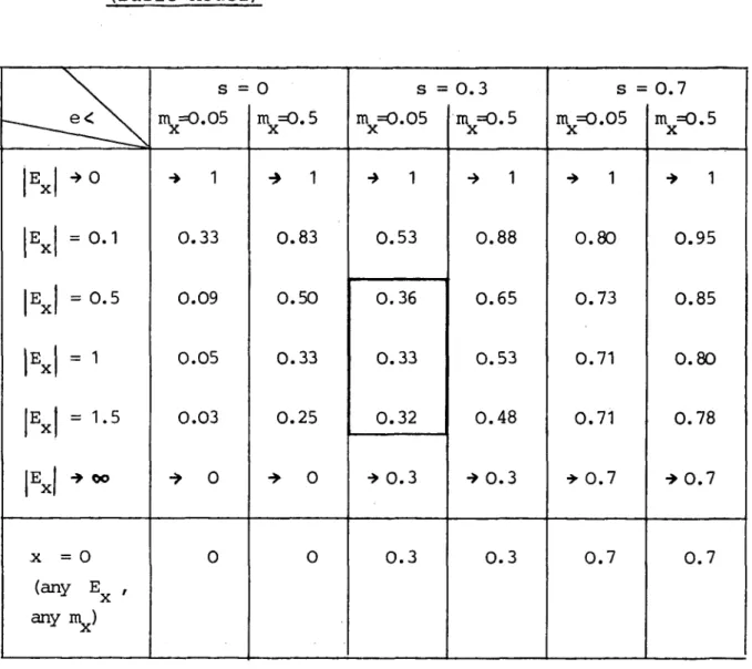
Let us put some numbers into inequality (56) to obtain a quantitative picture of the magnitude of the required efficiency gap. Table 1 presents a set of more or less realistic alternative values for the three parameters |E |, m and s with the corresponding "threshold" values of e.

X

The table reveals some interesting features:

- For r e a l i s t i c values of |E | (in the empirically confirmed T 4

range 0.5 ^ |E | ^ 1.5) , m (m ' = 0.05) ands (s = 0.3

X X X

which is roughly the average implicit subsidy rate in Germany under the present income tax law), government spending has to be about three times more efficient than private purchases; no doubt, such a gigantic efficiency gap simply does not exist in the.real world since even extreme monopsonistic power should at most yield a ten or a fifteen percent discount.

- Even for a pathologically low absolute value of E

(|E I = 0 . 1 ) and an equally pathologically high value of

X

m (m = 0 . 5 ) , we obtain quite substantial efficiency

X X

gaps, especially in the case of low (and realistic) subsidy rates.

- The sensitivity of the efficiency gap with respect to changes in the subsidy rate is high; in fact, s figures as the lower limit of e for |E | going to infinity; in the case of a corner solution with x = 0. at the outset, the threshold value of e just equals s.

4

See the survey by Clotfelter & Steuerle (1981) for the U.S., and Paque (1982) for Germany. Of course, empirical

estimates yield, uncompensated price elasticities; for

realistically low values of % i mx» 0 . 0 5 ) , however, we can

infer compensated elasticities which are, in absolute value, only slightly below the estimates of the uncompensated

Table 1: Threshold Efficiency Gaps for Selected Parameters (Basic Model) • — - ^ E X Ex Ex Ex Ex Ex X \ e< - - , •» 0 = 0. = 0. = 1 = 1. = 0 (any E any mx) 1 5 5 s = mx=0.05 -> 1 0.33 0.09 0.05 0.03 •> 0 0 0 0 . 0 . 0 . 0 . . 5 1 83 50 33 25 0 0 0 . 0 . 0 . 0 . •» 0 0 s = . 0 5 1 53 36 33 32 . 3 . 3 0 . 3 0 . 0 . 0 . 0 . •> 0 0 . 5 1 88 65 53 48 . 3 . 3 • » 0 . 0 . 0 . 0 . * 0 0 s = . 0 5 1 80 73 71 71 . 7 . 7 0 . 7 mx=0.5 * 1 0.95 0.85 0.80 0.78 , 0 , 0 . 7

All this points to the unambiguous policy conclusion that, under any realistic circumstances captured in our model, the government should use the instrument of subsidization or tax expenditures as much as possible.

22

-4. A Generalized Model

Our previous model was restrictive in one important sense: We assumed that all individuals have identical tastes and equal incomes. In the following we shall briefly sketch a possible generalization of this model to allow for individuals with differing tastes and incomes.

4.1. Model Specification and Comparative Statics

We assume an economy with two separate groups of consumers called K and J. Within each group all individuals are alike; between the groups they differ in all demand parameters and income. If present, externalities equally extend over both groups so that no "balkanization" of the economy into

homogenous groups is possible.

The f-consumption of an individual of group K and J respec-tively is now given by

(47) f

k

= £i+y(kn-1)J . x

k

+

and

(48) f

j

= jj1+}f(jn-1)] • x

j

+ }fknx

k

+ F l + ^ n - i ) ] - 3.

respectively, with the superscript k (j) denoting the rele-vant parameters and variables of group K (J), and small letter k (j) denoting the share of group K (J) in the total number of individuals (with k + j = 1 ) . Note that govern-ment spending is equally provided to all individuals, no matter which group they belong to.

The government budget constraint now reads as

(49) n Jt(kB

k

+ jB

1

') - sp(kx

k

+ jx^)J - epg = r ,

with price p and per-unit subsidy rate s being the same for all individuals.

Again, the comparative statics for our two policy options comprise two constraints, a consumption constraint and a budget constraint. The consumption constraint is now given by

( 5 0 ) k f + j f J I • d s + k f . + j f J • d t = 1

l _ s J s j |_ t t J

for policy option I, and

(51) jTkfgk + j f

g j

j - dg + fkftk + Jf

t DJ- dt = 1 for policy option II.

Note that equations (50) and (51) describe constraints for the economy as a whole, not for any single individual. With only two policy parameters (either s and t or g and t) at the disposal of government, it is not possible to uniquely determine individual consumption levels of f in the case of heterogenous individuals. For (partially) public goods

(1 > )f > 0 ) , such an economy-wide constraint makes much sense since for this kind of goods, social target levels are often formulated in aggregate terms. For purely private goods

( y = 0 ) , however, a specified aggregate consumption level is an odd social target so that the following analysis is of not much use for this particular case.

The budget constraints for our two policy options are given by totally differentiating equation (49) with respect to s (g)

and t yielding (52) d t TkBk + jB^ - s p ( k xt k + - pds / " s ( k xs k + j-Xg-*) + k xk + j x ^ J = 0 and (53) ndt JkBk + jBj - sp(kxt k + jx^) I - pdg fns(kx k + jx •*) + e l = 0

24

-parallel to our previous model: Equations (50), (52) and (51), (53) respectively can be solved for ds, dt and dg, dt respectively. Note that the assumed rational adjustment process of any individual's f-purchases x to changes in others' (or government's) provision of f is the same as before, with the only technical difference that the adjust-ment takes place with respect to changes of f-purchases inside and outside any individual's group. Analytically, this means that we specify two reaction functions - e.g. x = x (x ^) and x ^ = x -1 (x ) - which yield a unique

s s s i s s s

solution for x , x J as functions of the unobservable

de-s ks i k i

mand parameters ra , m J, E and E J (analogously for

x , x -* and x, , x,-*) . While the whole procedure involves some messy algebra, it does not pose any particular analytical difficulties.

4.2. The Main Results

Solving the above model for dt and dt in the unconstrained case, we obtain two cumbersome tax cost measures which are

+ +

presented as equations (1 ) and (2 ) in the appendix. To focus on the effect of differences in the demand parameters between the two groups, we make some simplifying assumptions;

k i k i

in particular, we assume that B = BJ = B and x = xJ = x and

we let the total number of.individuals n go to infinity (thus restricting the analysis to the practically relevant large number case). Under these assumptions, we end up with two limiting tax cost measures - corrected for the degree of externalities - which read

(54) llm and r T dt1 L B

~

L

x

r f

P (e-s)(1-s)Jf(k(1-m

k

)+j(1-m

j

(55) limldt^fi+^n-i)}! =

L

^

respectively. As i t turns out,

lim [ d t

1

{ 1+)f ( n - 1 ) ] ] > l i m f d t

1 1

f i + y ( n - 1 ) j ] i f f

( 5 6 ) e <

k i k i

which - for m = m = m and E = E J = E - boils down to

X X X X X X

inequality ( 4 5 ) .

k i k i In the case of a corner solution with x = x J = x = x J =

k i 9 5 = x = x J = 0, the results of our previous model with

iden-tical tastes and equal incomes are only slightly modified. k i

Without any additional restrictions on B , BJ and n, the two

tax cost measures are given by T sp 1 (57) d tA = r- r > 0, and 1 + f (n-1) kBK + jBD II ep . 1 • (58) dt: = •—T- r > 0 so that 1 + f (n-1) k BK + jBJ •

dt > dt iff e < s which is a mere replication of inequality (46).

Returning to the unconstrained case, we have to ask the

question whether inequality (56) does in any way invaliditate the conclusions drawn on basis of our previous, more restrictive model. To make the two threshold levels of e as given by

inequalities (45) and (56) comparable, we assume that both the average marginal propensity to spend on x and the average com-pensated price elasticity of demand for x are the same in both models, i.e.

26

-(59) in = km k + jmJ , and

Thus the two threshold levels are normalized to the same average level of the demand parameters. Substituting equa-tions (59) and (60) into equation (45), it turns out that the previous model requires a lower e, i.e. a higher fiscal efficiency gap to compensate for the intrinsic superiority of policy option I, iff

(61) -A- > -^ for y > 0 ,

IP. E -1 x x k i

with m > mJ by assumption (without loss of generality).

For y = 0, the threshold level of e is the same in both models. As long as there is no conclusive empirical

evidence of a positive correlation between m andJE |- and, 5 x x

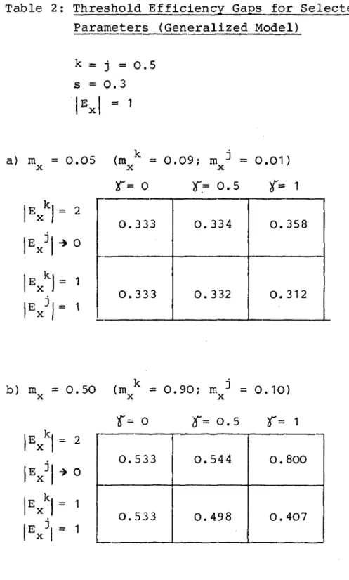
so far, there is none-, the odds are in favour of in-equality (61) to hold. Even if inin-equality (61) does not hold, however, the upward correction of the threshold level of e is likely to be very small. This can be inferred

from Table 2a) which depicts a scenario of somewhat realistic parameters (k=j = 0 . 5 ; s = 0 . 3 ; |E I = 1; m = 0.05) to

demonstrate the effect of different group specific parameters. Even in the most unfavourable case (Jf= 1; |E | = 2; JE -1 j •» 0) ,

the threshold level of e is only about 2.5 percentage points above its level for the coresponding case with

iden-tical tastes (with e 0.333). Only when we switch to a pathologically high average marginal propensity to spend on x (m = 0.5), we obtain - at least in one of the pure public good cases - a marked upward correction of e (see Table 2b)). All this points to the conclusion that the presence of dif-ferent demand parameters can hardly challenge our prior con-clusions. Even with heterogeneous individuals, the widest possible use of tax expenditures is appropriate on efficiency grounds.

Table 2: Threshold Efficiency Gaps for Selected Parameters (Generalized Model)

k = j = 0.5 s = 0 . 3 E a) m = 0 . 0 5 (m k = 0 . 0 9 ; m ^ = 0 . 0 1 ) X X X

o

x 0.333 0.333 0.334 0.332 0.358 0.312 b) m = 0 . 5 0 (in k = 0 . 9 0 ; raj* = 0 . 1 0 ) X X X ; m -* = x = o ?r= 0 . 5 j r = 1 E K X E

x

3 P i ExD = 2 -> 0 = 1 0. 0. 533 533 0. 0. 544 498 0. 0. 800 407

28

-4.3. Who Should Be Subsidized?

After having established a case for tax expenditures, we are left with the question of how a tax expenditure system should be designed in a world with heterogeneous individuals In particular, we can now address the interesting question whether differences in price elasticities of demand for the

favoured good justify varying per-unit subsidy rates on efficiency grounds.

To tackle this problem, we compare three policy options, namely

(i) a subsidy increase granted to all individuals at the same rate, i.e. ds # 0, dt * 0;

(ii) a subsidy increase granted only to the group of in-dividuals with a high compensated price elasticity E (say, group k) , i.e. ds 4= 0, dt * 0;

(iii) a subsidy increase granted only to the group of in-dividuals with a low compensated price elasticity E (say, group j ) , i.e. ds-3 4= 0, dt * 0.

To isolate the effect of differences in E , we assume

1 '

m = m -1 = m to be equal for all individuals •

After proceeding, with minor changes, along the analytical lines described above, we obtain three tax-cost measures for the unconstrained case, namely

(62) dt(l) =

p (1-s)f]oc

k

+jx^ji+,f(n-1) (1-m )?+sfkx

k

(m -E ^H-jx^m -E

:

. k -J I . XJ *- x x x x •* ^ o

1+Hn-i) -n(kBk + jB^) (kxk E k + jx^ E i)

-n(kBk + jBD) E

(iii) ( ) f 3 ( ) ( )} + s-(m-E

j

)

(64) d t

u i i ;

= •

l

J U

x x

> o.

-n(kBK + jBD) E ]

As it turns out, our assumption that |E | > \E^\ is necessary and sufficient to ensure that d t ^1 1 1^ > d t ^ > d t *i : L* . Hence

tax cost minimization requires the marginal subsidy increase to be granted only to group K, i.e.- to the group of high elasticity demanders of x. Note, that income differentials are irrelevant for marginal per-unit subsidization: As long as income is a poor proxy for the compensated price .elasticity, the present system of tax deductions in the U.S. and Germany - with per-unit subsidization increasing with marginal tax rates - lacks an efficiency rationale.

In the case of corner solutions with x = xJ = 0, all three

are given by measures (65) dt d t( j H L ), dt s p H)T(n-1 a n d 1 ) k Bk + d t i B ^ (iii) > 0 .

Not surprisingly, price elasticities do not matter in this case since there is no intramarginal subsidization to be financed; thus all options are equally efficient at the margin.

Our critique of the tax deduction system is entirely

different from the critique by Hochman & Rodgers (1977) who base their analysis on Lindahl-optimality criteria.

30

-5. Concluding Remarks

Our analysis has shown that, under a broad range of realistic circumstances, a tax expenditure is preferable to direct

government spending as an instrument to reach some target level of collective consumption. Taken at face value, this result has remarkable consequences for economic policy making; it may even contain the germ for a redefinition of the

function of governments. Given our results, we are inclined to confine any government - be it local or national - to the limited task of deciding which prices of which goods should be artificially lowered so as to ensure that some politically determined target level of collective consumption will be reached. Pushing our model to its logical extreme, we may even conceive of a government setting up a tax expenditure scheme which allows all political target levels of consump-tion to be reached simultaneously without any actual tax revenue.

Note that, in this vision of a "tax-free state", we do not preclude the public authorities from exercising a more or less tight legal control on the kind.of good provided by private agents. But setting up a legal control framework and financing an activity is quite a.different matter: Even such a classical public good as national defense may be ex-clusively financed through private donations at an appropri-ately high per-unit subsidy rate. Of. course, the tighter the public control, the less it makes sense to speak of a genuine private provision. Hence the most fertile ground for tax expenditures may still lie in the traditional realm of private charities (e.g. in education, the arts, health

services and social relief) where the kind of goods to be pro-vided is not too narrowly specified by some public authority.

How should a tax expenditure system be designed to be most efficient? Without tackling the details of this welfare

theoretic question , we may conjecture that an efficient scheme should be organized on a firmly decentralized basis. Most so-called public goods are public only with respect

to a narrow geographical area - say, a town or a region -, and the people who are potentially willing to pay for these goods live in or fairly close to that area. Thus local governments are likely to be much better informed about preferences and demand parameters of the citizens of their region than any central authority; in optimizing the struc-ture of a tax expendistruc-ture system, they should clearly have a comparative advantage. Needless to say that the present systems of income tax deductions for charitable contributions

(such as Sec. 170 Internal Revenue Code in ,the U.S. and § 10b Income Tax Law in Germany), do. not conform to this decentralization postulate. Hence drastic reforms.are re-quired: While the central government may., fix some flat-rate income tax credit for charitable contributions in general, the local governments should be given the authority to grant additional per-unit tax exemptions for particular charitable contributions with special interest to the community. These per-unit exemptions may (and should) vary among regions and goods and possibly even among donors (whenever price

elasticities of demand differ significantly). Induced income tax revenue losses of the central government.should be accounted for in the calculation of interregional grants so that any single local government has an incentive to choose a scheme which minimizes the cost to all governments taken together.

To force bureaucrats to use the efficient instrument of tax ex-penditures instead of maximizing direct government spending, a constitutional amendment should be passed which prohibits

governments on all levels to resort to direct government spending as long as the public support to private voluntary

The author is presently working on a detailed analysis of this point. The following remarks are a sketchy summary of his conclusions.

32

-good supply is the less expensive policy.option. Clearly, such an amendment would lay the ground for a dramatic ex-pansion of the private charity market. With a good deal of tax money ready to be channelled into the voluntary non-profit sector, a large number of new charities and founda-tions would appear to compete for private contribufounda-tions. Such a pluralistic system of competitive public good pro-vision would probably be much more efficient in coping with changing economic and social conditions than the present system of a rigid monopolistic bureaucracy.

Finally, the proposed system has a distinct advantage in granting the taxpayers a much more effective voice in de-termining the structure and volume of public services, even without a change of the government in power. If, e.g.,

charity x does not conform to the expectations of its donors - be it for mismanagement or simply for a change in consumer preferences -, its level of donations will decrease. In this situation, the government has two options: either it lets the demand shift determine a new equilibrium level of x's activity (which means that consumers are sovereign even in public goods provision!) or it raises the subsidy up to the point where the charity is back at its previous level of donations (which means that a high level of transparency is introduced into public decision making). In any case, we would be better off than in the present system.

X X X X T (1 ) d t

-.s) (kx

k

+jx

j

)fi + rl(kn1) ( 1

-i

n-D n (kB

k

+jB

j

){kx

k

[i-f(1-m

j

)] [-E

k

] + j

y(1-ni

j

)] [m

k

-E

k

]+jx

j

ri-(Bkxj-Bjxk) +

1 e. [1 -f

2

(.1 -m

k

) (1 -m

j

.)] .+. (1 -m

k

) f 1 -J(.1 -m

j

)j £j-jkn (e-s) -e] -skn (1 -y)j .+.

Jf(n-1) n (1-e) [kB

k

m

k

{i-f(1-m

j

)J+jB

j

m

j

{i-f(1-m

k

)

j

JT(.1-m

k

)] [)f [ j n ( e - s ) - e ] - s j n ( 1 - p j

U)

34

-References

Clotfelter, Charles T., C. Eugene Steuerle (1981), "Chari-table Contributions", in: H.J. Aaron, J.A. Pechman

(eds.), How Taxes Affect Economic Behaviour. Washington D.C., pp. 403-446.

Feldstein, Martin (1980), "A Contribution to the Theory of Tax Expenditures. The Case of Charitable Giving", in: H.J. Aaron, H.J.. Boskin (eds.), The Economics of

Taxation. Washington D . C , pp. 99-122.

Hochman, Harold M., James D. Rodgers (1977), "The Optimal Tax Treatment of Charitable Contributions", in:

National Tax Journal 30., pp. 1-18.

Paque, Karl-Heinz (1982), "The Efficiency of Public Support to Private Charity. An Econometric Analysis of the

Income Tax Treatment of Charitable Contributions in the Federal Republic of Germany". Kiel Working Paper No. 151 Ramsey, Frank P. (1927), "A contribution to the Theory of