arXiv:2006.10478v1 [math.PR] 18 Jun 2020
SHADOW MARTINGALES – A STOCHASTIC MASS TRANSPORT APPROACH TO THE PEACOCK PROBLEM
MARTIN BRÜCKERHOFF MARTIN HUESMANN NICOLAS JUILLET
Abstract. Given a family of real probability measures(µt)t≥0increasing in convex order (a peacock) we describe a systematic method to create a martingale exactly fitting the marginals at any time. The key object for our approach is the obstructed shadow of a measure in a peacock, a generalization of the (obstructed) shadow introduced in [12, 45]. As input data we take an increasing family of measures
(να)
α∈[0,1] withνα(R) =αthat are submeasures ofµ0, called a parametrization of
µ0. Then, for anyαwe define an evolution(ηαt)t≥0of the measureνα=η0αacross our peacock by settingηα
t equal to the obstructed shadow ofναin(µs)s∈[0,t]. We identify
conditions on the parametrization(να)α∈[0,1]such that this construction leads to a unique martingale measureπ, the shadow martingale, without any assumptions on the peacock. In the case of the left-curtain parametrization(νlcα)α∈[0,1]we identify the shadow martingale as the unique solution to a continuous-time version of the martingale optimal transport problem.
Furthermore, our method enriches the knowledge on the Predictable Representa-tion Property (PRP) since any shadow martingale comes with a canonical Choquet representation in extremal Markov martingales.
Keywords: peacock problem, peacocks, optimal transport, martingale optimal trans-port, predictable representation property, Choquet representation
Mathematics Subject Classification (2010): Primary 60G42, 60G44; Secondary 91G20.
1. Introduction
Two finite measuresµandµ′ onRwith finite first moments are said to be in convex order, denoted by µ≤c µ′, if
R
ϕdµ≤R
ϕdµ′ for all convex ϕ:R→ R. Peacocks are families (µt)t≥0 of probability measures on R with finite first moments that increase in convex order. Given a peacock (µt)t≥0, the peacock problem is to construct a probability measure π such that the canonical process X = (Xt)t≥0 is a martingale w.r.t. its natural filtration and the marginal distributions coincide with (µt)t≥0, i.e. Lawπ(Xt) =µt for eacht≥0.
There is a wide range of beautiful solutions to this problem employing different ideas and techniques, e.g. [39, 42, 14, 37, 27, 43, 34, 22, 2, 36, 24]. On the one extreme, there is the fundamental non-constructive result of Kellerer [39] proving the existence of Markov solutions for any given peacock. On the other end of the spectrum, there are very explicit constructions for specific sub classes of peacocks, many of which can be found in the monograph [26] by Hirsch, Profeta, Roynette, and Yor. However, it
Date: June 19, 2020.
MB and MH have been partially supported by the Vienna Science and Technology Fund (WWTF) through project VRG17-005; they are funded by the Deutsche Forschungsgemeinschaft (DFG, Ger-man Research Foundation) under GerGer-many’s Excellence Strategy EXC 2044 –390685587, Mathematics Münster: Dynamics–Geometry–Structure. NJ thanks the Erwin-Schrödinger Institue (ESI) for sup-porting his stay in Vienna in June 2019.
is difficult to manage both aspects by constructing an explicit solution for a generic peacock. Only recently there have been contributions in this direction by Lowther [42], Hobson [27], Juillet [36] and Henry-Labordere and Touzi [25].
We propose a new method to systematically construct a martingale associated with a peacock. Thereby, we rely on the rich theory of optimal transport. In optimal transport a coupling of two probability measures is interpreted as a plan to transport one marginal to the other one. More precisely, given a coupling π of two probability measures µ0 and µ1 on R, i.e. a probability measure π onR2 withπ(A×R) =µ0(A) and π(R×B) = µ1(B) for all Borel sets A and B. The quantity π(A×B) can be interpreted as the amount of mass (of the measure µ0) that is transported from the set
A to the set B under π. Conversely, a coupling π is fully characterized by the family of values(π(A×B))A,B and this characterization still holds if we only consider certain
families of sets, e.g. only sets A×B withA of the type (−∞, q]. Note, that given q
the values of B 7→π((−∞, q]×B) are encoded in the second marginal of π|(−∞,q]×R ,
i.e. in the measure ηq :=π((−∞, q]× ·). Therefore, the family (ηq)q∈R associated with
((µ0)|(−∞,q])q∈R, i.e. the one-step evolution (µ0((−∞, q]), ηq), completely determines the transport planπ.
In recent years, this mindset of optimal transportation found several new applica-tions within stochastic analysis sometimes subsumed under the name stochastic mass transport, see e.g. [13, 6, 18, 41, 8]. In various striking applications it turned out to be useful to interpret a stochastic process X ≡(Xt)t≥0 as a device to transport mass from time0 to the distribution ofX at a (potentially random) time τ. To identify the induced coupling of the distribution of X at time0 and time τ it is then necessary to trace the evolution of fixed parts of the initial distribution, e.g. to consider for A⊂R
the evolution in tof
ηAt :=P[Xt∈ ·|X0 ∈A].
Observe, that opposed to the classical optimal transport setup knowing the evolution of ηAt for A ⊂ R does in general not allow to recover the process X. Note that this
already fails for two-step processes. For instance, compare the law of (X1, X2, X3) where the three random variables are independent and identically distributed to the law of (X1, X2, X2).
We call a measureν a submeasure ofµ, ifν≤+µ, i.e. ifν(A)≤µ(A)for all measur-able sets A. For instance, the restrictions (µ0)|A of µ0 =Law(X0) to the measurable setsA= (−∞, q]are submeasures ofµ0. Using this terminology, the goal of this article is to uniquely define a martingale associated with a peacock(µt)t≥0 from the following input data only:
• A parametrization of µ0, i.e. a family of submeasures (να)α∈[0,1] of µ0 s.t.
να(R) =α, να≤
+νβ for α≤β, and ν1 =µ0.
• For each α, the evolution of να through the marginals (µt)
t≥0, i.e. a family
(ηα
t)t≥0 of submeasures of(µt)t≥0,ηtα≤+µtfor allt≥0, satisfyingνα=ηα0 ≤c ηα
s ≤c ηαt for all 0≤s≤t. These evolutions also need to be consistent in the
sense that ηα
t ≤+ηβt for all α≤β in[0,1] andt≥0.
It is easy to see that, without further assumptions, this data is not sufficient to uniquely determine the law of a martingale. It turns out that a certain convexity of
(να)α∈[0,1] together with some kind of minimality in the choice of(ηα)α∈[0,1] is the key to uniquely define a martingale measure via this procedure.
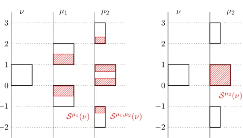
−2 −1 0 1 2 −2 −1 0 1 2 Figure 1. The shaded area shows the evolution (ηαt)t≥0 ofνα through
(µt)t≥0 for α = 31 (left) and α = 23 (right), respectively. Here µt =
Unif[−1−t,1+t] and Iα = [−α,+α]. The measures are represented by their density functions w.r.t. the Lebesgue measure. The representation is in 3D-perspective with times evolving transversally to the page.
Before introducing the appropriate notions we would like to present our solution in a special setting which already gives a good idea of the general case (namely Theorem 1.5 in Subsection 1.1):
Corollary 1.1. Let(µt)t≥0 be a peacock. For any nested family of intervals (Iα)α∈[0,1]
for which
(i) µ0(Iα) =α for any α∈[0,1],
(ii) α7→R
Iαydµ0(y) is a convex function and
(iii) supIα <+∞ and∂Iα∩∂Iβ =∅ for all α 6=β in [0,1],
there exists a unique solution π to the peacock problem w.r.t. (µt)t≥0 such that for any
other solution ρ to the peacock problem w.r.t.(µt)t≥0 it holds
(1.1) Lawπ(Xt|X0∈Iα)≤cLawρ(Xt|X0∈Iα)
for all α∈[0,1]and t≥0. Moreover, (X0, Xt)t≥0 is a Markov process underπ.
Remark 1.2. As the reader should have noticed, a completely rigourous statement of
Corollary 1.1 requires to specify on which measurable space the martingale measure π
in Corollary 1.1 is defined. Here, as well as in all of the paper, we use R[0,∞) with the
Borel σ-algebra induced by the product topology on R[0,∞).
Alternatively, if the map t 7→ µt is right-continuous w.r.t. the weak topology (cf.
Section 3.1), by standard martingale regularization (see e.g. [46, II §2]) there exists
a càdlàg modification of the canonical process on R[0,∞) under π that one can use to
define the solution π directly on the Skorokhod space of càdlàg functions from [0,∞) to
R, see Section 6 for an implementation.
Consider the peacock (µt)t≥0 consisting of uniform distributionsµt= Unif[−1−t,1+t] on the intervals[−1−t,1 +t]and the interval familyIα = [−α, α],α∈[0,1]. It is not difficult to check that this pair satisfies the conditions (i)-(iii) in Corollary 1.1 and for two choices of α, Figure 1 illustrates the evolution (ηα
t)t≥0 of να = (µ0)|Iα over time
under the solution to the peacock problem constructed in Corollary 1.1.
We would like to highlight a few features of Corollary 1.1 which all appear in the general case, Theorem 1.5, again:
• The parametrization ofµ0 induced by the intervals Iα, namely(µ0|Iα)α∈[0,1], is in a certain sense convex, cf. item (iii) in Corollary 1.1.
• The minimality condition (1.1) affects only the conditional one-dimensional marginal distributions underπ. Thus, only the evolutionηα
t =αLawπ(Xt|X0 ∈
Iα) of να = (µ
0)|Iα is prescribed by the requirement to be minimal in convex
order but (a priori) no joint distributions are fixed.
• In particular, (1.1) says that Lawπ(Xt|X0 ∈ Iα) is minimal in convex order among all solutions to the peacock problem, for every α. Explicitly, for every
t, every α, every convex function ϕ, and any other solution ρ to the peacock problem w.r.t.(µt)t≥0 there holds
Z
ϕ dLawπ(Xt|X0 ∈Iα)≤ Z
ϕ dLawρ(Xt|X0 ∈Iα),
so that, in this precise sense,Lawπ(Xt|X0 ∈Iα) is as concentrated as possible. Hence, we can think of π as a plan to transport µ0|Iα through (µt)t∈[0,1] as concentrated as possible subject to the martingale constraint.
• Finally, it will become apparent during the proof of Theorem 1.5 that the Markov property turns out to be a consequence of the fact thatLaw(X|X0) is uniquely determined by its marginal distributions, see Lemma 4.29, Proposition 4.30.
1.1. Main results. Our main results, Theorem 1.5 and 1.6, enlarge the perspective presented in Corollary 1.1 but are of the same nature. They in fact permit further parametrizations of µ0 and stress the optimal feature of our shadow martingales.
To state Theorem 1.5 we need to introduce the objects that will replace the specific parametrization(µ0|Iα)α∈[0,1] and property (1.1). We start with the definition of shad-ows, the concept that will replace (1.1). To not overload the introduction we give a preliminary (but correct) definition and refer to Proposition 4.20 where it is extended to a more general setting.
As before a martingale measure is a probability measure under which the canonical process is a martingale w.r.t. the filtration generated by the process.
Definition 1.3. For all peacocks (µt)t≥0, t ≥0 and ν ≤+ µ0 with α =ν(R) >0 the
set
αLawπ(Xt) : π is a martingale measure, ν =αLawπ(X0)
andαLawπ(Xs)≤+µs for all s∈[0, t]
attains a minimum w.r.t. the convex order ≤c. This minimum is called the shadow of
ν in (µs)s∈[0,t] and is denoted bySµ[0,t](ν).
We say that two finite measuresµandµ′onRwith finite first moments are in
convex-stochastic order, denoted byµ≤c,s µ′, ifR
ϕdµ≤R
ϕdµ′ for all convex and increasing functionsϕ:R→R. A parametrization (να)
α∈[0,1] ofµ0 is called≤c,s-convex if for all α1< α2 < α3 in[0,1]it holds (1.2) ν α2 −να1 α2−α1 ≤c,s να3 −να2 α3−α2 .
Since property (1.2) can be interpreted as increasing slopes of secant lines for the func-tionsα7→R
ϕdµα,ϕincreasing and convex, this property is called≤
c,s-convexity. The
following three parametrizations, that were introduced in [13] for one step processes, are examples of ≤c,s-convex parametrizations (cf. Lemma 4.6 for the proof):
• the left-curtain parametrization
νlcα=µ0|(−∞,F−1
µ0(α))+ (α−µ0(−∞, F −1
where F−1
µ0 is the quantile function of µ0, i.e the generalized inverse of the cumulative distribution functionFµ0,
• the sunset parametrization να
sun =αµ0 for everyα ∈[0,1]and
• the middle-curtain parametrization
νmcα =µ0|(qα,q′
α)+cαδqα+c ′ αδq′
α
where qα ≤ qα′ and cα, c′α ∈ [0,1] are chosen such that να
mc(R) = α and R ydνα mc(y) = R ydµ0(y).
We remark that ifµ0has no atoms the left-monotone and the middle-curtain parametriza-tions are special cases of the parametrization used in Theorem 1.1. In particular, the parametrization in Figure 1 is the middle-curtain parametrization of the uniform mea-sure on[−1,1].
The final object that we need to introduce are martingale parametrizations. Their purpose is to allow conditioning on the initial behaviour of a martingale which is not of the form{X0 ∈Iα}for some Borel setIα⊂R. Again, as Definition 1.3, Definition 1.4 is a simplified version of the general Definition 4.1. Notice that the notion of submeasure from page 2 is also well-defined for measurable spaces other than R. Moreover, we denote by πα(Xt∈ ·) the push-forward measure of πα via Xt (it is a measure of mass α).
Definition 1.4. Let (να)
α∈[0,1] be a parametrization ofµ0 and π the law of a
martin-gale indexed by [0,∞). A family (πα)
α∈[0,1] of finite measures is called a martingale
parametrization of π w.r.t. (να)α∈[0,1] if
(i) for every α∈[0,1] it holdsπα(R[0,∞)) =α,
(ii) we have πα≤
+πα ′
for all α≤α′,
(iii) for every α∈(0,1]the measure πα
α is a martingale measure,
(iv) we have π1 =π and
(v) it holds πα(X
0 ∈ ·) =να for all α∈[0,1].
As we discuss in Subsection 4.1.2, a martingale parametrization (πα)α∈[0,1] w.r.t.
(να)
α∈[0,1] is a convenient way of encoding that for each α ∈ [0,1] the martingale π transports the submeasureναofµ
0according toπα, i.e. we may interpretπαformally as “αLawπ(X|X0 ∈να)”. In particular, any martingale parametrization (πα)α∈[0,1] w.r.t.
(να)α∈[0,1] induces a specific evolution ofνα for everyα∈[0,1], namely ηαt =πα(Xt∈ ·). We would like to stress that there might be several martingale parametrizations of
π w.r.t.(να)
α∈[0,1] (cf. Example 4.9). We can now state our first main result:
Theorem 1.5. Let (µt)t≥0 be a peacock and (να)α∈[0,1] a ≤c,s-convex parametrization
of µ0. Then, there exists a unique pair (π,(πα)α∈[0,1]) where the martingale measure π
solves the peacock problem w.r.t.(µt)t∈T, (πα)α∈[0,1] is a martingale parametrization of
π w.r.t. (να)
α∈[0,1] and
(1.3) πα(Xt∈ ·) =Sµ[0,t](να)
for all α ∈[0,1] and t≥0. We call π the shadow martingale (measure) w.r.t. (µt)t≥0
and (να)α∈[0,1].
The shadow martingale π can be represented as π = Law MU
where U is a [0,1]
-valued random variable and (Ma)a∈[0,1] is a family of R[0,∞)-valued random variables
(i) {U} ∪ {Ma:a∈[0,1]} is a collection of independent random variables,
(ii) the random variableU is uniformly distributed on[0,1]withLaw(MU
0 |U ≤α) = 1
ανα for all α∈(0,1]and
(iii) for each a ∈ [0,1], (Ma
t)t≥0 is a Markov martingale which is uniquely
de-termined by its (one-dimensional) marginal distributions, i.e. any martingale
(Yt)t≥0 withLaw(Yt) = Law(Mta) for all t≥0 satisfies Law(Y) = Law(Ma).
Note that the single constraint on π given by (1.3) only involves the evolution
(πα(Xt ∈ ·))t≥0 of the submeasures να and a priori no joint distributions. Hence, the theorem states that taking a ≤c,s-convex parametrization of the initial marginal µ0 and fixing its evolution to be as concentrated as possible w.r.t. the convex order uniquely characterizes a martingale.
Specializing to the left-curtain parametrization(να
lc)α∈[0,1]and additionally assuming that both µ0 has no atoms and t 7→ µt is weakly right-continuous, we can give an alternative characterization of the associated shadow martingale which identifies it as a unique solution to a variant of an optimal transport problem, namely a peacock version of the martingale optimal transport problem:
Theorem 1.6. Let (µt)t≥0 be a peacock with µ0({x}) = 0 for all x ∈ R and c a
sufficiently integrable and regular cost function with ∂x∂2yc <0 (cf. Theorem 8.4). The
shadow martingale πlc w.r.t. (µt)t≥0 and (νlcα)α∈[0,1] is the only solution to the peacock
problem w.r.t. (µt)t≥0 that satisfies
(1.4) Eπlc[c(X0, Xt)] = inf{Eρ[c(X0, Xt)] :ρ sol. to peacock problem w.r.t.(µt)t≥0}
simultaneously for all t≥0.
The necessity of the assumption of no atoms is best seen by looking at the case
µ0 = δ0. In that case, since the marginals at time t are given, each solution to the peacock problem w.r.t. (µt)t∈[0,1] is a solution to the optimization problem (1.4).
When considering only finitely many marginals {µt0, µt1, . . . , µtn}increasing in con-vex order, and a corresponding piecewise constant peacock, Theorem 1.6 reduces to a recent theorem by Nutz, Stebegg and Tan [45, Theorem 7.16]. As we will prove in Remark 8.6, in certain situations the martingale measureπlcis the unique limit of these
piecewise constant martingales.
Remark 1.7. Corollary 1.1, Theorem 1.5 and Theorem 1.6 are well-defined and valid
if we replace the index set [0,∞) by an abstract totally ordered set (T,≤) with minimal
element 0∈T (see Corollary 7.5, Theorem 7.3 and Theorem 8.4).
Moreover, the convex-stochastic order is defined via the integrals of increasing convex functions. Of course, one could define an analogue order relation on the set of finite measures via decreasing convex functions. Then the corresponding version of Theorem 1.5 for a “convex-decreasing”- parametrization of the initial marginal distribution holds.
1.2. Choquet representation and the PRP property. There is another abstract point of view on our main result Theorem 1.5. Any martingale measure has a Choquet representation, i.e. it can be written as a superposition of martingale measures that are extremal elements of the convex set of all martingale measures. Such a representation is interesting because the extremality in the set of all martingale measures naturally relates to the predictable representation property (PRP). In stochastic analysis a mar-tingale M is said to satisfy the PRP if and only if any martingale X adapted to the natural filtration of M can be represented as a stochastic integral with respect toM.
According to a theorem by Jacod and Yor a martingale satisfies the PRP if and only if it’s law is extremal in the convex set of all martingale measures (cf. [32, 48, 31]). Hence, any martingale measure is a superposition of martingales with the PRP. To the best of our knowledge, no concrete recipe for the construction of such a representation is known. However, for shadow martingales there exists a natural Choquet representa-tion. In fact, this natural Choquet representation is the driving force behind the proof of Theorem 1.5, especially the uniqueness part.
Given a peacock µ = (µt)t≥0, our construction of the uniquely determined shadow martingale starts with a representation of µas a superposition of peacocks, i.e.
(1.5) µ=
Z
[0,1]
ηa da.
This representation is induced by the shadow and the choice of a proper parametrization
(να)
α∈[0,1] ofµ0 (cf. Lemma 5.4). The peacocksηa in (1.5) are in general not extremal in the convex set of all peacocks (in the sense that 2ηa =η′+η′′ impliesη′ =η′′=ηa)
so that (1.5) cannot be called a Choquet representation of µ. However, they satisfy a very similar property that we call non self-improvable (NSI) (cf. §4.3):
(1.6) 2ηa=η′+η′′ and η0′ =η0′′=η0a implies η′ =η′′=ηa.
The main consequence of the NSI property is that for every peacock that satisfies this property there exists only one martingale measure that is associated with this peacock. Thus, the unique martingale measures πa associated withηaare extremal in the set of
martingale measures with fixed initial distribution, i.e. (
2πa=ρ′+ρ and
ρ′(X0 ∈ ·) =ρ′′(X0 ∈ ·) =πa(X0 ∈ ·)
implies ρ′ =ρ′′=πa
Indeed, if ρ′ and ρ′′ are two martingale measures with 2πa = ρ′ +ρ′′ that have the
same initial distribution as πa, the marginal distributions of these three objects satisfy (1.6) and thus the marginal distributions of ρ′ and ρ′′ are ηa, i.e. they coincide with
the marginal distributions of πa. But then the uniqueness of the associated martingale measure given by the NSI property yields πa = ρ = ρ′. The superposition of these
special martingale measures
(1.7) π=
Z 1 0
πada
is exactly the shadow martingale w.r.t. µ and (να)
α∈[0,1]. More precisely, πa is the distribution of Ma in the representationπ = Law(MU)of the shadow martingale that is described in the second part of Theorem 1.5.
The representation of the shadow martingale in (1.7) is in general not yet a Cho-quet representation because the martingale measures πa are only extremal in the set
of martingale measures with fixed initial distribution. Nevertheless, we can directly obtain a Choquet representation from (1.7) and then by Jacod and Yor’s theorem we have a rather explicit representation of the shadow martingale as a superposition of martingales that satisfy the PRP. In the case of the left-curtain parametrization, this is particularly easy. The construction of (1.5) is such that for each α∈[0,1] there holds Rα
0 η
a
0da = νlcα where (νlcα)α∈[0,1] is the left-curtain parametrization. Looking again at the definition of (νlcα)α∈[0,1] in Subsection 1.1, we see that η0a is a Dirac measure for any a ∈ [0,1]. Hence, the peacocks ηa and the associated martingale measures πa
Therefore, in the case of the left-curtain parametrization, (1.7) is in fact already a Choquet representation of the shadow martingale π. More generally, given any ≤c,s -convex parametrization (να)
α∈[0,1] of µ0 we obtain a Choquet representation of the shadow martingale by further disintegrating (1.7) w.r.t. the initial marginal µ0, i.e. by conditioning on the starting value of π.
We want to emphasize that this Choquet representation of the shadow martingale is uniquely determined by the representation of the peacockµgiven in (1.5). This repre-sentation ofµis constructed using only the shadow and a≤c,s-convex parametrization of the initial distribution. To show that the peacocks (ηa)
a∈[0,1]in (1.5) satisfy the NSI property (which is very similar to extremality, cf. (1.6)) is in fact a crucial part of our proof. Moreover, this abstract point of view of our result makes it apparent that the construction of the shadow martingale is purely based on its marginals as an object in the space of peacocks and thus these are intrinsic solutions to the peacock problem. 1.3. Outline. There are several contributions to martingale optimal transport theory and the peacock problem that are related to our results and that we discuss in Section 2. In Section 3 we recall order relations for finite measures and important properties of the peacock problem.
In Section 4 we introduce (martingale) parametrizations, (general obstructed) shad-ows and non self-improvable peacocks. These concepts are not only essential ingredients of our proof of Theorem 1.5 but are interesting in themselves.
In Section 5, we prove a variant of Theorem 1.5 in the case that the peacock is indexed by a countable set S⊂[0,∞) that contains 0 and satisfies supS ∈S. In this setup it is possible to avoid some of the technicalities needed to be able to handle the general case and concentrate on the key steps and ideas of the proof. Let us briefly sketch them in the following paragraphs:
We need to construct a family of measures (πα)
α∈[0,1] on RS that satisfies both Definition 1.4 (i)-(iii) and property (1.3)1and need to show that this family is uniquely determined by these two properties (note that (1.3) already implies that π := π1 is a solution of the peacock problem w.r.t. (µt)t∈S and that condition (v) of Definition 1.4
is satisfied). To this end, we pursue the following approach:
• STEP 1: Any family of measures(πα)
α∈[0,1] on RS satisfies Definition 1.4 (i)-(iii) if and only if there exists a family of martingale measures(ˆπa)
a∈[0,1] such that πα = Z α 0 ˆ πada
for allα∈[0,1]. In particular, the family(πα)
α∈[0,1]is uniquely determined by any such family(ˆπa)
a∈[0,1] and for Lebesgue-a.e.a∈[0,1]it holds
(1.8) πˆa= lim
h↓0
πa+h−πa h
under an appropriate topology (cf. Subsection 3.1). Thus, (πα)
α∈[0,1] satisfies property (1.3) if and only if the following two properties hold: For Lebesgue-a.e.
a∈[0,1] and allt∈S the limit (1.9) ηˆat = lim
h↓0
Sµ[0,t]∩S(νa+h)− Sµ[0,t]∩S(νa) h
1Of course withR[0,∞)replaced byRSand[0
exists and the distribution of Xt under πˆa is ηˆa
t. Step 1 is accomplished in
Subsection 5.1.
• STEP 2: Step 1 implies that there exists a family(πα)
α∈[0,1] with the desired properties, if there exists a family (ˆπa)
a∈[0,1] of martingale measures on RS such that the canonical process under ˆπa has marginal distributions (ˆηa
t)t∈S
for Lebesgue a.e. a∈[0,1]. By Kellerer’s Theorem, for fixed a∈[0,1] such a martingale measureπˆa exists if (ˆηa
t)t∈S is a peacock. Using the calculus rules
that we develop for general obstructed shadows, we show in Subsection 5.2 that for Lebesgue-a.e.a∈[0,1]the limit in (1.9) exists and that(ˆηa
t)t∈S is a peacock. • STEP 3: Another implication of Step 1 is that the family (πα)
α∈[0,1] con-structed in Step 2 is uniquely determined if there exists only one martingale measure with marginal distributions (ˆηa
t)t∈S for Lebesgue a.e. a ∈ [0,1].
Un-fortunately, just from the defining equation (1.9), the peacock(ˆηa
t)t∈S does not
need to satisfy this very restrictive property for all a∈ [0,1] where (ˆηa t)t∈S is
defined (cf. Example 9.4).
That being said, it is sufficient for us that (ˆηat)t∈S is NSI for
Lebesgue-a.e. a ∈ [0,1] since the NSI property implies the uniqueness of a martingale associated with(ˆηta)t∈S(cf. Section 1.2). To show this, we introduce an auxiliary
optimization problem and establish a corresponding monotonicity principle (cf. Subsection 5.3). The minimality of the shadow in conjunction with the ≤c,s -convexity of(να)
α∈[0,1]implies that(ˆηa)a∈[0,1]is a minimizer of this optimization problem which in turn implies that(ˆηa
t)t∈S is NSI for Lebesgue-a.eaas desired
(see Subsection 5.4).
IfS was finite, we could use the concept of Kellerer dilations as in [13] to show that for alla∈[0,1]where(ˆηa
t)t∈S is well-defined there is only one martingale measure with
these one-dimensional marginal distributions (cf. Remark 4.31). However, as shown in Example 9.4, this is not true if S is infinite. This major difference between the case of a finite index set and a countable infinite one, is the reason why we have to develop new tools and techniques and cannot extend methods used in [13] and [45].
In Section 6 we establish Theorem 1.5 in the setting of a continuous time index set
T ⊂[0,∞)under the additional assumption that the given peacock is right-continuous. Martingale regularization techniques imply that martingale measures are uniquely de-termined by their behaviour on a countable index set. We will show in Subsection 6.2 that also the obstructed shadow and the NSI property are determined by the be-haviour of the peacock (µt)t∈T restricted to a well chosen countable index set S ⊂T.
This allows us to lift the results from Section 5 to the setting of T ⊂ [0,∞) with right-continuous peacock.
In Section 7 we show how we can pass to an abstract totally ordered index set without any assumptions on the peacock. In particular, this completes the proof of Theorem 1.5 (recall that it was stated for the totally orderd space T = [0,∞)). Moreover, we explain how Corollary 1.1 follows from Theorem 1.5.
The proof of Theorem 1.6 is contained in Section 8.
Finally, in Section 9 we discuss counterexamples regarding shadows and NSI peacocks and provide explicit examples of shadow martingales.
2. Related literature
The theory of optimal transport dates back to Monge (1781) and Kantorovich (1939) and has a huge variety of different facets and applications (see e.g. [47]). Martingale op-timal transport is a relatively new part of this theory, that has for instance applications in robust mathematical finance (see e.g. [1] or the book [23]). Given two probability measures µ0 and µ1 with µ0 ≤c µ1 and a cost function c, the goal is to minimize (or maximize)
π 7→Eπ[c(X0, X1)]
over the set of couplings of µ0andµ1 that additionally satisfy the martingale property. Among the solutions of the problem (for different cost functions) are the couplings presented by Hobson and Neuberger [29], Hobson and Klimmek [28] and for other related problems the couplings recently introduced in [33] by Jourdain and Margheti and in [13] by Beiglböck and Juillet. Note that martingale optimal transport problems are a special case of a wider class of transport problems as weak optimal transport problems [20, 19] or linear transfers [16].
The left-curtain coupling introduced by Beiglböck and Juillet in [12] is of partic-ular importance for our approach of the peacock problem. Besides being the unique minimizer for a certain class of cost functions (cf. [12]), the left-curtain coupling has several different characterizations, for instance concerning the geometry of its support [35] or in the context of the Skorokhod Embedding problem [10, 13]. Moreover, Hobson and Norgilas show in [30] that it possesses a natural interpretation in Mathematical Finance.
The concept of shadow – that is at the root of this article – is introduced and developed in the same paper [12] as the left-curtain coupling π. In fact,πis introduced by
π(X0≤a, X1 ∈ ·) =Sµ1(µ0|(−∞,a]).
for every a ∈ R. The shadow martingale w.r.t. the left-curtain parametrization is a natural extension of this coupling (and hence also of its discrete time extension by Nutz, Stebegg and Tan in [45]) to the continuous time case. Moreover, shadow martingales extend the concept of shadow couplings introduced in [13].
The name peacock (alias PCOC) which is derived from the French term Processus
Croissant pour l’Ordre Convexe and likewise the peacock problem were introduced by
Hirsch, Profeta, Roynette and Yor in their monograph [26] and are therefore quite re-cent. However, the construction of martingales that match given marginal distributions at least goes back to the seminal work of Kellerer [39]. Since then a variety of solutions have been developed before it was subsumed under the name peacock problem. Most of these solutions make more or less restrictive additional assumptions on the peacock, e.g. assuming that the peacock satisfies the (IMRV) property (see [43]) or consists of the marginal distributions of a solution to a certain class of SDE (see [21]). Moreover, the construction of fake Brownian motions (e.g. [2, 22]) can be seen as solutions to a (very specific) peacock problem. The monograph [26] provides a comprehensive overview of solutions to the peacock problem that work with special classes of peacocks.
Recently there were several contributions that face generic peacocks without a rich additional structure. There is the solution of Hobson [27] which is based on the Sko-rokhod Embedding Problem and the one of Lowther [42] who constructs for continuous peacocks with connected support a solution under which the canonical process is a strong Markov process. The approach closest to our class of solutions is the one par-allely studied by Henry-Labordère, Tan and Touzi [24] and Juillet [36]. The shadow
martingale w.r.t. the left-curtain parametrization (να
lc)α∈[0,1]is the limit of the discrete time simultaneous minimizer of
Eπ[c(X0, Xtk)] ∀ 1≤k≤n among all martingale coupling of µ0, µt1, . . . , µtn for allcwith∂x∂
2
yc <0asntends to
infinity for a suitable chosen sequence of nested finite partitions ofT whose mesh tends to zero. In contrast, the solution of [24, 36]– when it exists– is constructed as the limit of the concatenation of the discrete time simultaneous minimizers of
Eπ[c(Xtk−1, Xtk)] ∀ 1≤k≤n.
for allcwith∂x∂2yc <0. Unsurprisingly, this solution behaves notably differently than
the shadow martingale induced by the left-curtain parametrization (see Example 9.10). Besides this article we are not aware of solutions to the peacock problem that are related to shadow martingales w.r.t. a parametrization which is not the left-curtain one. Similarly, there are no results about uniquely constructing martingales by solely describing how parts of the initial distribution evolve. In fact, the only approach in this direction that we are aware of is [15] but in a non-martingale setup.
3. Preliminaries
In this section we introduce our notation and recall objects and properties that are well known in the context of martingale optimal transport and the peacock problem. Since we want to work at the level of probability distributions (of processes), we some-times choose a non-standard perspective on standard results.
3.1. Notation. We denote byM0(X)(resp.P0(X)) the set of all finite measures (resp. probabilty measures) on some measurable space X. The underlying space will mostly be the space of functions from T to R, denoted by RT, for some totally ordered set
(T,≤). In this case, the space RT is equipped with the product topology and the corresponding Borelσ-algebra, the canonical process onRT is denoted by (Xt)t∈T, i.e.
for all t∈T
Xt:RT ∋ω7→ω(t)∈R,
and (Ft)t∈T is its natural filtration defined by Ft=σ(Xs :s≤t).
The setM1(RT)consists of allπ ∈ M0(RT)for which all one-dimensional marginal distributions have a finite first moment. We equip M1(RT) with the initial topology generated by the functionals (If)f∈G0∪G1 where
If :M1(RT)∋π 7→ Z RT fdπ ∈R and ( G0 ={g◦(Xt1, . . . , Xtn) :n≥1, t1, . . . , tn∈T, g∈Cb(R n) } G1 ={|Xt|:t∈T}.
We denote this topology on M1(RT) by T1. In contrast, we denote by T0 the initial topology onM0(RT)that is generated by the functionals(If)f∈G0 only. The subspace of
probability measures inM1(RT)is denoted byP1(RT)and equipped with the inherited topology. IfT is finite, the topology onP1(RT)is induced by the1-Wasserstein metric
W1,l1 corresponding to the l1-metric onRT (see Villani [47, Theorem 6.9]). It is also not difficult to see, that, if T is countable, M1(RT) is first countable and therefore continuity is equivalent to sequential continuity.
Note now that we can reduceG0 in the defintion ofT0 to the following set of functions
G′
0={ω∈RT 7→1} ∪ {g◦(Xt1, . . . , Xtn) :n≥1, t1, . . . , tn∈T, g∈Cc(R n)}
To see this, recall that a sequence (πn)n∈N converges to π w.r.t. some initial topology T defined by some set of functions G if and only if (If(πn))n∈N converges to If(π) in
Rfor allf ∈ G. IfT is finite and Gcontains Cc(RT), the same limit is also satisfied for any continuous function f that can be dominated by a linear combination generated with elements fi ∈ G, i.e such that
|f| ≤X i
ζifi.
This is the reason why (i) the topology generated by G0′ is exactly T0 (also if T is infinite), (ii) functions g◦(Xt1,· · ·, Xtn)where ggrows at most linearly at infinity are
admissible for T1.
We denote the push-forward of a measure π ∈ M1(RT) under some measurable map f defined on RT by f#π. Ifπ is a probability distribution, we refer to the push-forward as the law or distribution of f underπ denoted byLawπ(f). Furthermore, the
expression “marginals of a probability measure π on RT”, always refers to all the one-dimensonal marginal distributions of the canonical process underπ, i.e. to the measures
Lawπ(Xt) for t∈T.
LetS be a subset of T and projS :RT →RS the projection on the index setS. The induced projection map
M1(RT)∋π7→(projS)#π∈ M1(RS)
is continuous w.r.t. T1 on M1(RT) and M1(RS). We denote the measure π projected on the coordinates in S, i.e. (projS)#π, by the shorter notation π|S as if it were the
restriction of a random vector.
Moreover, we denote the cumulative distribution function of a probability measure
µ onRby Fµ and its quantile function is
Fµ−1:α∈[0,1]7→inf{x∈R:Fµ(x)≥α}.
We also denote byλthe Lebesgue measure on[0,1], by UnifI the uniform distribution
on an interval I ⊂R and byδx the Dirac measure at pointx.
3.2. Order relations and potential functions. We use several partial order rela-tions on M1(R). They can all be introduced in a parallel way saying thatµ∈ M1(R) is smaller than or equal to µ′ ∈ M
1(R)if (3.1) Z R ϕdµ≤ Z R ϕdµ′
for every ϕ in a certain positive cone of measurable test functions. These orders and the corresponding cones are:
• The positive order: µ≤+µ′ if (3.1) holds for all non-negative ϕ.
• The convex order: µ≤c µ′ if (3.1) holds for all convexϕ.
• The convex-positive order: µ≤c,+µ′ if (3.1) holds for all non-negative convex
ϕ.
• The convex-stochastic order: µ≤c,s µ′if (3.1) holds for all increasing convexϕ.
Both non-negative and convex functions are bounded from below by an affine func-tion and thus, since the first moments are finite, the integrals in (3.1) are well-defined with values in (−∞,∞]. Note that the positive order is well-defined for finite measures
on any measurable space (e.g.RT). Moreover, recall from the introduction that we call
π a submeasure of π′ if π ≤
+π′.
Lemma 3.1. Let µ andµ′ be in M
1(R).
(i) If µ≤c µ′, then µ(R) =µ′(R) and RRydµ(y) =RRydµ′(y).
(ii) If µ≤c,+µ′ andµ(R) =µ′(R) , then µ≤c µ′.
(iii) If µ≤c,sµ′ and R
Rydµ(y) =
R
Rydµ′(y), then µ≤cµ′.
Proof. Item (i): The four functionsx7→ ±1and x7→ ±xare convex functions.
Item (ii): If µ ≤c,+ µ′ and µ(R) = µ′(R), equation (3.1) is satisfied for every non-negative convex function and also for x 7→ −1. Thus (3.1) is satisfied for any convex function that is bounded from below. Hence, for a general convex function ϕ with R
Rϕdµ′<+∞, (3.1) holds forϕn=ϕ∨(−n)and the monotone convergence theorem
shows that (3.1) holds for ϕas well.
Item (iii): We use a similar argument adding x 7→ −x to the set of nondecreasing convex functions. Any convex function is the pointwise increasing limit of a sequence of convex functions with limit slope bounded at −∞.
Lemma 3.2. Let µn, µ′n, µ, µ′ ∈ M1(R) for all n∈N.
(i) Suppose(µn)n∈N and(µ′n)n∈N converge toµ and µ′ under T0. Ifµn≤+µ′n for
all n∈N, thenµ≤+µ′.
(ii) Suppose (µn)n∈N and (µ′n)n∈N converge to µ and µ′ under T1. For any order
relation≤c, ≤c,+ or≤c,s represented by ≤, the relationsµn≤µ′n for all n∈N
implyµ≤µ′.
Proof. Item (i): It is clearly sufficient to test the positive order by indicator
func-tions of closed intervals. For any such function ϕ there exists a sequence (ϕm)m∈N
of continuous bounded functions such that 0 ≤ϕm ≤ ϕfor all m ∈N and R
Rϕdµ =
limm→∞RRϕmdµ. Since convergence inT0 implies thatRRϕmdµ= limn→∞RRϕmdµn
for all m∈N, the claim follows.
Item (ii): For any (non-negative/increasing) convex functionϕ∈L1(µ), there exists a sequence(ϕm)m∈Nof (non-negative/increasing) convex functions with bounded slope
at±∞such thatϕm ≤ϕfor allm∈NandR
ϕdµ= limm→∞
R
ϕmdµ. Since the slope of ϕm is bounded, there exist am, bm>0such that |ϕm(x)| ≤am|x|+bm for allx∈R
and hence the claim follows because the sequences converge w.r.t. T1 (cf. Subsection
3.1).
Note that convergence inT0 does in general not preserve the order relations≤c,≤c,+ and ≤c,s. However, a sequence that is convergent under T0 and has a uniform upper bound in ≤c,+, is in fact convergent under T1:
Lemma 3.3. Let (µn)n∈N be a sequence in M1(R). If there exists a measure θ ∈
M1(R) such that µn ≤c,+ θ for all n ∈ N, then the sequence (µn)n∈N is uniformly
integrable, i.e. lim N→∞supn∈N Z R| x|1[−N,N]cdµn(x) = 0.
Hence, (µn)n∈N converges under T0 if and only if (µn)n∈N converges under T1.
More-over, if (µn)n∈N converges underT0 to µ∈ M1(R), then it holds
R
fdµn→R
f dµ for
Proof. We have|x|1[−N,N]c(x)≤(2|x| −N)+for all x∈RandN ∈N. Thus, we obain Z R| x|1[−N,N]cdµn(x)≤ Z R (2|x| −N)+dθ
and this upper bound converges to 0asN tends to infinity by dominated convergence. Similarly, for any convex function ϕ∈L1(θ) and continuous f with|f| ≤ϕit holds
Z R| f|1[−N,N]cdµn≤ Z R (ϕ+|x| −N)+dθ
for all N ∈ N. Hence, standard argumentation via the triangle inequality based on compact continuous functions coinciding with f on [−N, N] yields that R
fdµn →
R
f dµ asntends to infinity for all suchf.
Dealing with the convex order, potential functions are a very useful representation of finite measures on R. They are defined as follows:
Definition 3.4. Let µ∈ M1(R). The potential function of µ is the function
U(µ) :R∋x7→
Z
R|
y−x|dµ(y)∈R+.
Since elements of M1(R) have finite first moments, the potential function is always well-defined. We collect a few important properties of potential functions below.
Lemma 3.5 (cf. [12, Proposition 4.1]). Let m ∈ [0,∞) and x∗ ∈ R. For a function
u:R→Rthe following statements are equivalent:
(i) There exists a finite measure µ∈ M1(R) with mass µ(R) =m and barycenter
x∗ =R
Rxdµ(x) such that U(µ) =u .
(ii) The function u is non-negative, convex and satisfies
(3.2) lim
x→±∞u(x)−m|x−x ∗|= 0.
Moreover, for all µ, µ′ ∈ M1(R) we have µ=µ′ if and only ifU(µ) =U(µ′).
Convex ordering and convergence in M1(R) can be well expressed in terms of po-tential functions.
Lemma 3.6. For all µ, µ′ and sequences (µn)n∈N in M1(R) with µ(R) = µ′(R) =
µn(R) for all n∈N, we have the following properties:
(i) It holds µ≤c µ′ if and only if U(µ)≤U(µ′).
(ii) It holds µn→µ under T1 if and only if U(µn)→U(µ) pointwise.
Proof. Since for everyx∈Rthe function fx:y7→ |y−x|is convex the direct
implica-tion of (i) is obvious. The reverse implicaimplica-tion is part of the folklore (see e.g Exercise 1.7 of [26]). It can be proved as follows: let C be the cone of real functions f for which R
fdµ ≤ R
fdµ′. It includes the constants and also the functions fx, x ∈ R. Considering both sequences (f±n−n)n∈N, by the monotone convergence theorem we
obtain ±x∈C. Hence C contains any piecewise (we mean with finitely many pieces) affine convex function. By the monotone convergence theorem again we see that every convex function is in C.
Sincefxis affine close to±∞, the direct implication of (ii) is obvious. For the reverse implication, since all measures have the same finite mass and U(µn)(0)→U(µ)(0) we have R
f dµn →n∈∞ R
f dµ for x 7→ 1 and x 7→ |x|. Therefore it suffices to establish the convergence for every continuous and compactly supported functionf. Notice that
the vectorial space spanned by the functions fx and the constant functions includes the continuous and piecewise affine functions with compact support. Hence we can conclude by their density in Cc(R) for the uniform norm.
Specified to families monotonously increasing in convex-stochastic order, the second part of the previous lemma yields the following result.
Corollary 3.7. Let T ⊂ R and (µt)t∈T be a family in M1(R) that is increasing in
convex-stochastic order, i.e. µs≤c,sµt for all s≤t in T. There exists a countable set
S ⊂T such that t7→µt is a continuous map from T\S toM1(R) under T1.
Proof. For allq ∈Qthe function
(3.3) t7→U(µt)(q) = Z R |y−q|dµt(y) = 2 Z R (y−q)+dµt(y)− Z R (y−q) dµt(y)
is continuous except on a countable set Sq because it is the difference of two
func-tions that are monotonously increasing in t. Set S = S
q∈QSq. Observe that ut¯ :=
lims↓tU(µs) is a well defined convex function as a pointwise limit of convex functions.
This limit exists by monotonicity in tof the integrals in (3.3). Alsout(x) :=U(µt)(x)
is a convex function and we get ut¯ = ut on Q for all t 6∈ S. Since both ut¯ and
ut are continuous as convex functions this equality extends to R. Similarly, it holds
limr↑tU(µr)(x) = U(µt)(x) for all x ∈ R and t 6∈ S. Thus, the map t 7→ U(µt)(x)
is continuous for every x ∈ R at any time t 6∈ S. This transfers to the continuity of
t7→µtoutside of S by Lemma 3.6 (ii).
Despite monotonicity, a family increasing in convex-stochastic order does in general not admit left- and right-limits everywhere underT1. For instance, the family(µt)t∈[0,1] with µt= 1−t2 2−t2δ−1−1t + 1 2−t2δ1+t µ1=δ2 does not have a left-limit at 1.
3.3. Infimum and supremum in convex order.
Definition 3.8. Let A be a set of measures in M1(R). If A possesses a smallest
upper bound w.r.t. convex order, we call it the convex supremum of Aand denote it by
Csup A. It is then the unique measure ζ such that
(i) µ≤c ζ for all µ∈ A and
(ii) ζ ≤c ζ′ for all ζ′ that satisfy (i).
Similarly, we define Cinf A as the convex infimum, if it exists.
Proposition 3.9. Let Abe a non-empty subset ofM1(R) such that all measures in A
have the same mass and the same barycenter.
(i) The convex infimumCinfA exists.
(ii) If there exists some θ ∈ M1(R) such that µ ≤c,+ θ holds for all µ∈ A, then
the convex supremum CsupA exists.
Moreover, their potential functions satisfy
U(CinfA) = conv
inf
µ∈A U(µ)
and U(CsupA) = sup
µ∈A U(µ).
where conv(f) denotes the convex hull of a function f, i.e. the largest convex function
Proof. Item (i): Since the measures of A all have the same mass m and barycenter
x and U(mδx) is convex, the set {g : g convex, g ≤ infµ∈AU(µ)} is not empty. Let u be defined by u(x) = sup{g(x) : g convex, g ≤ infµ∈AU(µ)}. It is convex as the
pointwise supremum of convex functions and U(mδx)≤u≤U(µ)for any fixedµ∈ A.
Hence u posseses the right behavior at±∞ in the sense of Lemma 3.5. Therefore u is a potential function and the corresponding measure satisfies the properties of a convex infimum by Lemma 3.6 (i).
Item (ii): According to [12, Lemma 4.5] applied tomδxandθthe orderingmδx ≤c,+θ implies that there exists aθ′∈ M1(R)withmδx≤c θ′such that for allη∈ M1(R)with
mδx ≤c η ≤c,+θ there holds η ≤c θ′ (θ′ is a restriction of θin a proper neighborhood
of ±∞, up to atoms).
In particular, we obtain U(mδx)≤U(µ)≤U(θ′) for every µ∈ A and therefore the convex function u= supµ∈AU(µ) satisfies U(mδx)≤u≤U(θ′). Thus,u has the right
behavior at ±∞ in the sense of Lemma 3.5. Hence, by Lemma 3.5 u is a potential function and the corresponding measure satisfies the properties of a convex supremum
(see Lemma 3.6 (i)).
Remark 3.10. The assumption that all measures in A have the same mass and
barycenter is equivalent to the assumption that A has a lower bound w.r.t. the
con-vex order. Hence, we don’t need an additional lower bound in (i).
Lemma 3.11. Let(µn)n∈N be a sequence in M1(R).
(i) If µm ≤c µn for all n≤ m in N, then (µn)n∈N converges to Cinf{µn:n∈ N}
under T1.
(ii) If µn ≤c µm ≤c,+ θ for all n≤ m in N and some θ ∈ M1(R), then (µn)n∈N
converges to Csup{µn:n∈N} under T1.
(iii) If (µ′
n)n∈N is another sequence in M1(R) and both sequences are increasing
in convex-oder and are uniformly bounded from above in convex-positive order, then
Csup
µn+µ′n:n∈N = Csup{µn:n∈N}+ Csup
µ′n:n∈N .
Proof. With Proposition 3.9 and Lemma 3.6 we can rewrite this statement in terms of
sequences of real functions and then the statement is well known.
Lemma 3.12. Let A be a non-empty subset of M1(R) such that all measures in A
have the same mass, the same barycenter and are dominated by some θ ∈ M1(R) in
convex-positive order. If additionally for all µ1, µ2 ∈ A there exists some µ′ ∈ A such
that µ1 ≤cµ′ andµ2 ≤cµ′, then there exists an increasing sequence (µn)n∈N inA that
converges to CsupA under T1.
Proof. The potential function of CsupA is given by u = supµ∈AU(µ). For any q ∈
Q there exists a sequence (νkq)k∈N of measures in A such that for the corresponding
potential functions uqk=U(νkq) the sequence (uqk(q))k∈N converges to u(q).
Let (qn)n∈N be an enumeration of Q, setµ1 =ν1q1 and choose aµn ∈ A that is an upper bound in convex order to the finite set
{µn−1} ∪
νql
k : 1≤k, l≤n
which is possible by assumption. Thereby, we get an increasing sequence in A that satisfies limn→∞U(µn)(q) = u(q) for all q ∈Q. Since (µn)n∈N is increasing in convex
order, limn→∞U(µn)(x) = supn∈NU(µn)(x) for all x ∈R. Thus, supn∈NU(µn) and u
u(x)for allx∈Rand we can apply Lemma 3.6 (ii) to conclude that(µn)n∈Nconverges
to CsupA underT1.
3.4. Peacocks and Kellerer’s Theorem. In this section we introduce notation re-garding peacocks and martingale measures.
We fix a totally ordered index set(T,≤). As already indicated in Subsection 3.1, we are not working on the level of processes but with their distributions on the state space
RT. However, we would like to introduce the martingale property and the Markov property that are typically formulated for processes indexed by T and not probability measures on RT.
Definition 3.13. Let π ∈ P1(RT).
(i) We callπ a martingale measure if the canonical process (Xt)t∈T is a martingale
w.r.t. its natural filtration under π, i.e. if
Eπ[Xt | Fs] =Xs π-a.e.
for alls≤tinT. The set of all martingale measures on RT is denoted byMT.
(ii) The probability measure π is said to be Markov if the canonical process (Xt)t∈T
is a Markov process underπ, i.e. if
Eπ[1A(Xt)|Fs] =Eπ[1A(Xt)|Xs] π-a.e.
for all Borel sets A⊂R ands < t in T.
We equipMT with the topology inherited fromT1 onP1(RT)and the corresponding Borel σ-algebra. All subsets of MT are equipped with the subspace topology and subspace σ-algebra.2
By Jensen’s inequality, the marginal distributions (Lawπ(Xt))t∈T of a martingale
measure π form a family in P1(R) that is increasing in convex order. Recall from the introduction that those families are called peacocks:
Definition 3.14. We call a family(µt)t∈T inP1(R)a peacock, ifµs≤c µtfor alls≤t
and we denote by PT the set of all peacocks indexed by T. Moreover, we say that a
martingale measure π is associated with a peacock (µt)t∈T if Lawπ(Xt) = µt for all
t∈T.
Since all elements of a family of finite measures increasing in convex order have the same mass (not always 1) by Lemma 3.1 (i), they can therefore easily be rescaled to become peacocks. We equip PT with the inherited product topology on P1(R)T where each factorP1(R)is equipped withT1. The corresponding Borelσ-algebra is the product σ-algebra.
Definition 3.15. Let S ⊂ T and (µt)t∈S be a family in P1(R). By MT((µt)t∈S) we
denote the set of all martingale measures π ∈ MT satisfying Lawπ(Xt) = µt for all
t∈S.
Thanks to the following result we know precisely when MT((µt)t∈T)is not empty.
Proposition 3.16 (Kellerer Theorem [39, 40]). Let(µt)t∈T be a family in P1(R). The
following are equivalent:
(i) The family(µt)t∈T is a peacock.
2Recall that the Borelσ-algebra of the subspace topology coincides with the subspaceσ-algebra of
(ii) There exists a martingale measure π ∈ MT((µt)t∈T) which can moreover be
chosen to be Markov.
The existence of solutions to the peacock problem is also true for martingales on Rd
withd≥2 (cf. [26]) but it is still an open problem whether in this case the martingale can be choosen to be Markov. An extension to partially ordered sets of indices is possible but only in certain cases (cf. [34]).
4. Parametrizations, shadows, and NSI
The goal of this section is to introduce the three concepts that are crucial on the one hand for the construction of the shadow martingales, namely parametrizations and obstructed shadows, and on the other hand for the uniqueness of the shadow martingale measure, namely the NSI property, cf. Subsection 1.3.
Throughout this section we fix a totally ordered set(T,≤). 4.1. Parametrizations.
Definition 4.1. Let X be a measurable space and µ∈ P0(X). A family (µα)α∈[0,1] in
M0(X) is called a parametrization of µif
(i) µα(X) =α for all α∈[0,1],
(ii) µα ≤
+µα ′
for all α≤α′ in[0,1] and
(iii) µ1 =µ.
Each parametrization of a probability measureµcan be seen as an explicit coupling of
µwith a uniformly distributed random variable on[0,1]that is added to the probability space. Recall, that λdenotes the Lebesgue measure on[0,1].
Remark 4.2. Let Xbe a measurable space,µ∈ P0(X)and(µα)α∈[0,1] a family of finite
measures on X. The following are equivalent:
(i) The family(µα)
α∈[0,1] is a parametrization of µ.
(ii) There exists a couplingξ ofλandµwithξ([0, α]×B) =µα(B)for allα∈[0,1]
and measurable sets B ⊂E.
Clearly, the coupling ξ is uniquely determined by (µα)
α∈[0,1] and vice versa.
Lemma 4.3. Let Xbe a measurable space, µ, ν ∈ P0(X), (µα)α∈[0,1] a parametrization
of µ and (να)α∈[0,1] a parametrization of ν. If µα =να for all α in a dense subset A
of [0,1], then µα=να for all α∈[0,1] and, in particular,µ=ν.
Proof. Letα∈(0,1]and(αn)n∈Na sequence inAwithαn↑α. Remark 4.2 yields that
µα(B) = lim n→∞µ
αn(B) and να(B) = lim
n→∞ν αn(B)
for all measurable sets B⊂X.
Given a specific peacock, the degree of freedom in our construction (Theorem 1.5) is the choice of a parametrization of the initial marginal. Hence, our primary motiva-tion to consider general (non-interval based) parametrizamotiva-tions of probability measures is to enlarge the set of possible input choices. For instance, an initial distribution that contains atoms cannot satisfy condition (i) in Corollary 1.1. The concept of parametrizations allows us to break these atoms into a continuum of quantiles.
4.1.1. Convex parametrizations.
Definition 4.4. Let µ be in P1(R). A parametrization (να)α∈[0,1] of µ is said to be
≤c,s-convex if (4.1) ν α2−να1 α2−α1 ≤c,s να3 −να2 α3−α2 for all α1 < α2 < α3 in [0,1].
Since both sides of inequality (4.1) can be interpreted as the slopes of secant lines of α 7→ να on [α
1, α2] and [α2, α3], the inequality yields that α 7→ να is convex in this sense. Moreover, property (4.1) is equivalent to α 7→R
ϕdνα being convex for all
increasing convex functions ϕ:R→R.
Lemma 4.5. Let µ∈ P1(R) and (να)α∈[0,1] be a parametrization of µ. If there exists
a sequence of nested intervals (Iα)α∈[0,1] in R such that
(i) supIα <+∞ andsupp(να)⊂Iα for all α∈[0,1),
(ii) supp(να2 −να1)⊂I
α1c for all α1< α2 in [0,1]and
(iii) α7→R
Rydν
α(y) is convex,
then the parametrization (να)
α∈[0,1] is ≤c,s-convex.
Proof. For allα1< α2 < α3 in[0,1]the measure
¯
ν1,2:=
να2 −να1 α2−α1 is concentrated on Iα2 by (i) and
¯
ν2,3:=
να3 −να2 α3−α2
is concentrated on the closure of the complement Iα2c by (ii). Moreover, both of theses
measures are probability measures and their barycenters satisfy Z R yd¯ν1,2(y)≤ Z R yd¯ν2,3(y) because α 7→ R Rydν
α(y) is convex by property (iii). Let ϕ : R → R be a convex
increasing function. Since Iα2 is bounded from above, there exists an increasing affine function l(y) =ay+bwithϕ≤lon Iα2 andϕ≥lon Iα2c. Thus, we obtain
Z R ϕd¯ν1,2 ≤ Z R ld¯ν1,2 =a Z R yd¯ν1,2(y) +b ≤ a Z R yd¯ν2,3(y) +b= Z R ld¯ν2,3≤ Z R ϕd¯ν2,3 because a≥0.
Note that this Lemma includes the setting of Corollary 1.1. Figure 4.1.1 illustrates the following three ≤c,s-convex parametrizations:
Lemma 4.6. The following parameterizations of µ∈ P1(R) are≤c,s-convex:
(i) The left-curtain parametrization (νlcα)α∈[0,1] with
νlcα =µ|(−∞,F−1
µ (α))+ (α−µ[(−∞, F −1
να sun νmcα να lc Figure 2. A sketch of να
lc,νmcα and νsunα for α∈ {14,12,34,1}.
(ii) The middle-curtain parametrization (νmcα )α∈[0,1] with
νmcα =µ|(qα,q′
α)+cαδqα+c ′ αδq′
α
forqα ≤q′αinRandcα, c′α∈[0,1]such thatνα
mc(R) =αand R ydνα mc= R ydµ.
(iii) The sunset parametrization (να
sun)α∈[0,1] withνsunα =αµ.
Proof. For item (iii), we have α 1
2−α1(να2 −να1) =µfor allα1< α2 in[0,1].
For item (i) and item (ii) we can apply Lemma 4.5 because both α 7→ R
Rydν α lc(y) and α7→R Rydν α
mc(y) are convex functions. Indeed, it holds 1 α2−α1 Z R ydνα2 lc − Z R ydνα1 lc ≤Fµ−1(α2)≤ 1 α3−α2 Z R ydνα3 lc − Z R ydνα2 lc
for all α1 < α2< α3 in[0,1] andα7→RRydνmcα (y) =
R
Rydµis constant.
4.1.2. Probability measures onRT. To be able to describe the evolution of a submeasure of the initial measure under a measure π ∈ MT we need to consider parametrizations of π as well.
Definition 4.7. Let π in P1(RT).
(i) Let (να)
α∈[0,1] be a parametrization of the initial marginal Lawπ(X0). A
fam-ily (πα)
α∈[0,1] in M1(RT) is called a parametrization of π w.r.t. (να)α∈[0,1] if
(πα)
α∈[0,1] is a parametrization of π withπα(X0∈ ·) =να for all α ∈[0,1].
(ii) A parametrization (πα)
α∈[0,1] of π is called a martingale parametrization of π,
if α1πα ∈M
T for all α∈(0,1].
Remark 4.8. Letπbe inP1(RT)and(να)α∈[0,1]be a parametrization of the initial
mar-ginal Lawπ(X0). Moreover, let (πα)α∈[0,1] be a parametrization of π w.r.t. (να)α∈[0,1].
It is not difficult to prove that for any α ∈ [0,1], for which there exists a Borel set
A⊂R withνα= (µ
Remark 4.8 suggests that we can interpretπα as the way να is transported underπ,
i.e. we can see πα(X
t∈ ·) as a formal version of ‘αLawπ(Xt|X0 ∈να)’. However, one has to be careful with this informal notation because contrarily to αLawπ(X|X0 ∈A) that is uniquely defined, there can be several parametrizations (πα)
α∈[0,1] of the same measure π w.r.t. (να)α∈[0,1], each giving another meaning to αLawπ(Xt|X0 ∈ να). This is illustrated in Example 4.9 just below. Hence, the correct interpretation of the existence of a parametrization(πα)
α∈[0,1]ofπw.r.t.(να)α∈[0,1]is thatνα = Lawπα(X0)
can be transported according to πα as part of the dynamic given byπ.
Example 4.9. Let (µt)t≥0 be a peacock, (νsunα )α∈[0,1] be the sunset parametrization of
µ0 and let π ∈ P1(R[0,∞) be associated with (µt)t≥0. Let (πα)α∈[0,1] be a (martingale)
parametrization of π w.r.t. (νsunα )α∈[0,1]. For α ∈ [0,1], set ρα = π−π1−α. Assume
that there is α¯ ∈ (0,1) such that πα¯ 6= ρα¯. Then, the family (ρα)
α∈[0,1] is again a
(martingale) parametrization of π w.r.t. (να
sun)α∈[0,1] but different from(πα)α∈[0,1]. For
a concrete example one can choose (µt)t≥0, π and (πα)α∈[0,1] as in Example 9.11.
Remark 4.10. In the last example the assumption that there is a martingale
parametriza-tion satisfying πα¯ 6= ρα¯ for some α¯ ∈ [0,1] is always satisfied as soon as the peacock
is not NSI (see § 4.3). NSI peacocks are extremal elements in the set of peacocks with
fixed initial marginal so that they are in a certain sense rare (see Lemma 4.28).
4.2. Shadows. The concept of the shadow of a measure ν through a family of finite measures is at the center of our construction (cf. Section (1.3)). After recalling pre-vious results of Beiglböck and Juillet [12] and Nutz, Stebegg and Tan [45] for simple and finitely obstructed shadows, we establish in Proposition 4.20 the existence of an obstructed shadow in the generality required for our setup.
4.2.1. The simple shadows. We start by recalling the original concept of (simple) shad-ows developed in [12]. Given two finite measures ν andµon R, the shadow ofν inµis defined as the minimum in convex order among all submeasure ofµthat are in convex order larger than ν. More precisely:
Proposition 4.11 (cf. [12, Lemma 4.6]). Let ν, µ∈ M1(R) satisfyingν ≤c,+µ. There
exists a unique finite measure η such that
(i) ν≤c η,
(ii) η≤+µand
(iii) for all η′∈ M
1(R) withν ≤c η′ ≤+µit holds η≤c η′.
The measure η is denoted by Sµ(ν) and called the shadow of ν in µ.
For a detailed proof we refer to [12]. We only stress that the proof is based on potential functions and the potential function of the shadow has an explicit expression in terms of the potential functions of ν and µstated in the following lemma:
Lemma 4.12. Letν, µ∈ M1(R) withν ≤c,+µ. It holds
U(Sµ(ν)) =U(µ)−conv(U(µ)−U(ν))
where conv(f) denotes the convex hull of a function f, i.e. the largest convex function
that is pointwise smaller than f.
Proof. This formula has been brought to our attention by Mathias Beiglböck and can

![Figure 3. The striped red area on the left represents the shadow of ν 1 = δ 0 in µ 1 = 2Unif [−1,1] and the shaded area on the right illustrates the shadow of ν 2 = Unif[ − 1 2 , 12 ] in µ 2 = Unif [−2,−1] + Unif [1,2] .](https://thumb-us.123doks.com/thumbv2/123dok_us/1967718.2791637/22.892.196.692.110.291/figure-striped-represents-shadow-unif-shaded-illustrates-shadow.webp)