University of California, Berkeley
U.C. Berkeley Division of Biostatistics Working Paper Series
Year Paper
Avoiding Boundary Estimates in Linear Mixed
Models Through Weakly Informative Priors
Yeojin Chung∗ Sophia Rabe-Hesketh† Andrew Gelman‡ Jingchen Liu∗∗ Vincent Dorie††
∗University of California, Berkeley, [email protected] †University of California, Berkeley, [email protected]
‡Department of Statistics, Columbia University, [email protected] ∗∗Columbia University, [email protected]
††Columbia University, [email protected]
This working paper is hosted by The Berkeley Electronic Press (bepress) and may not be commer-cially reproduced without the permission of the copyright holder.
http://biostats.bepress.com/ucbbiostat/paper284 Copyright c2012 by the authors.
Avoiding Boundary Estimates in Linear Mixed
Models Through Weakly Informative Priors
Yeojin Chung, Sophia Rabe-Hesketh, Andrew Gelman, Jingchen Liu, and Vincent Dorie
Abstract
Variance parameters in mixed or multilevel models can be difficult to estimate, especially when the number of groups is small. We propose a maximum penal-ized likelihood approach which is equivalent to estimating variance parameters by their marginal posterior mode, given a weakly informative prior distribution. By choosing the prior from the gamma family with at least 1 degree of freedom, we ensure that the prior density is zero at the boundary and thus the marginal posterior mode of the group-level variance will be positive. The use of a weakly informative prior allows us to stabilize our estimates while remaining faithful to the data.
A non-degenerate estimator for hierarchical variance parameters via
penalized likelihood estimation
Yeojin Chung∗, Sophia Rabe-Hesketh†
∗†Graduate School of Education, University of California, Berkeley, CA 94705, USA †Institute of Education, University of London
Vincent Dorie, Andrew Gelman, and Jingchen Liu
Department of Statistics, Columbia University, New York, NY 10027, USA
February 13, 2012 Abstract
We propose a maximum penalized likelihood approach for estimating group-level variance parameters in mixed or multilevel models, equivalent to estimating variance parameters by their posterior mode, given a weakly informative prior distribution. By choosing the prior from the gamma family with shape parameter greater than 1, we ensure that the estimated variance will be positive. When the maximum likelihood estimate is at zero, our maximum penalized likelihood estimator is approximately one standard error from zero and thus remains consistent with the likelihood while being non-degenerate. (In contrast, lognormal and inverse-gamma penalty functions effec-tively bound the estimated variance parameter away from zero, which can result in regularized estimates that are inconsistent with the likelihood.) We also discuss the use of the gamma family to convey substantive prior information. In either case—pure penalization or prior information—our recommended procedure gives non-degenerate estimates when the number of groups is small and in the limit coincides with maximum likelihood as the number of groups increases.
Keywords: Hierarchical Linear Model, Multilevel Model, Penalized likelihood, Variance
Estimation
§The research reported here was supported by the Institute of Education Sciences (grant R305D100017)
and the National Science Foundation (SES-1023189), the Department of Energy (DE-SC0002099), and Na-tional Security Agency (H98230-10-1-0184).
1
Introduction
Linear mixed models (e.g. Harville, 1977; Laird and Ware, 1982), also known as hierarchical or multilevel linear models, are widely used for longitudinal data, cross-sectional data on sub-jects nested in neighborhoods or institutions (hospitals, schools, firms), cluster-randomized trials, multi-site trials, and meta-analysis. The models include random intercepts and some-times random coefficients that vary among groups and that we will refer to as varying intercepts and coefficients. We consider the situation where some variability is known to exist a priori due to omitted group-level covariates. Maximum likelihood is a useful way to estimate variance parameters in mixed models. But when the number of groups is small, estimates of group-level variance parameters can be noisy and can often be zero. In a multi-variate setting, estimated covariance matrices can be singular. Estimating a variance to be zero causes underestimation of uncertainty in the parameter estimates of the model.
Most clearly, degenerate variance estimates lead to complete shrinkage of predictions for new and existing groups and yield estimated prediction standard errors that understate uncertainty. For example, Gelman et al. (2007) fit a multilevel model predicting voter choice given income, with the intercept and slope for income varying by state. They found that richer voters tended to support Republican candidates but with a slope that varied depending on some state-level predictors. For one election year, the fitted model had a zero value for the point estimate of the variance of the state-level errors for the slopes. In the resulting inferences, the state-level slopes were perfectly predicted by the state-level predictors. There is no reason to believe this—the perfect prediction is merely an artifact of a variance estimate that happened to be zero—and it is awkward to graph these results, showing an estimated perfect fit that we do not and should not believe. A related difficulty arises when comparing instances of a model that is repeatedly fit to similar data from different surveys or different years, yielding zero variance estimates some of the time.
When a variance parameter is estimated as zero, there is typically a large amount of uncertainty about this variance. One possibility is to declare in such situations that not enough information is available to estimate a multilevel model. However, the available alternatives can be unappealing since, as noted above, discarding a variance component or setting the variance to zero understates uncertainty. The other extreme is to fit a regression with indicators for groups (a fixed-effects model), but this will overcorrect for group effects (it is mathematically equivalent to a mixed-effects model with variance set to infinity) and also does not allow predictions for new groups.
If zero variance is not a null hypothesis of interest, a boundary estimate, and the corre-sponding zero likelihood ratio test statistic, should not necessarily lead us to accept the null hypothesis and to proceed as if the true variance is zero. This point is particularly important when zero variance leads to the smallest possible standard errors for parameters of interest as in random-effects meta-analysis where the practice of using tests of homogeneity as a ba-sis for choosing between fixed and random-effects meta-analyba-sis has been criticized (Hardy and Thompson, 1998; Curcio and Verde, 2011; Draper, 1995, p.52-53). Inclusion of varying intercepts can be viewed as a continuous model expansion (Draper, 1995) to allow for the possibility that there may be unexplained differences between groups (see also Gelman and Meng, 1996).
An argument against avoiding boundary estimates is that negative variance parameters should be permitted if the model is viewed as a marginal model for the responses given the covariates, in which case only the sum of the group-level and within-group variance must be positive (Verbeke and Molenberghs, 2000, p.52-53). However, we take a hierarchical perspective, where the intercepts vary due to omitted group-level variables, and therefore the group-level variance must be nonnegative.
Several authors (e.g., Kubokawa and Tsai, 2006; Srivastava and Kubokawa, 1999; Mathew and Niyogi, 1994; Kelly and Mathew, 1994) have developed nonnegative (definite) estimators
of variance components to improve standard estimation methods such as analysis of variance, maximum likelihood (ML) or restricted maximum likelihood (REML) in terms of Stein loss or mean-squared error (MSE). Our estimators are developed to avoid boundary estimates while respecting the data, and they turns out to perform as well as the standard methods such as ML or REML in terms of MSE.
1.1 Outline of our approach
In this paper we develop a non-degenerate estimator by maximizing the likelihood∗multiplied
by a penalty function, or equivalently by assigning a prior distribution to the unknown variance parameters and finding the posterior mode. It is possible to do this without requiring strong prior knowledge. But our functional form is general enough that it can also be applied when real prior information is available.
Our primary aim is to develop a default penalization that gives non-degenerate variance estimators in multilevel models, bounded away from zero but automatically respecting the data. In particular, we recommend a class of gamma priors (for unidimensional problems) and Wishart (for multidimensional) that produce maximum penalized likelihood estimates (or Bayes modal estimates) approximately one standard error away from zero when the maximum likelihood estimate is at zero. We consider these priors to be weakly informative in the sense that they supply some direction but still allow inference to be driven by the data. The prior has little influence when the number of groups is large or when the data are informative about the variance.
Penalized likelihood estimation has been used to obtain more stable estimates of item parameters in item response theory (Swaminathan and Gifford, 1985; Mislevy, 1986; Tsu-takawa and Lin, 1986) and to avoid boundary estimates in log-linear models (Galindo-Garre
∗We use the term likelihood to refer to the integrated or marginal likelihood, with random effects
et al., 2004) and latent class analysis (Maris, 1999; Galindo-Garre and Vermunt, 2006). To our knowledge, this idea has not previously been applied to variance parameters in multilevel models.
Compared with full Bayes or posterior mean estimation, our approach does not require simulation and is computationally as efficient as maximum likelihood estimation, in fact potentially more efficient as it avoids the slow convergence that can occur if the maximum likelihood estimate is on the boundary. No additional convergence checking is required and there is no need to specify priors for all model parameters. We have implemented posterior modal estimation in Stata and R with only minor modifications of existing software for max-imum likelihood estimation of linear mixed models. Given user-specified or default choices of hyperparameters, the programs automatically find the posterior mode of the variance parameter and provide inferences for the coefficients conditional on that estimate.
Although our main objective is to avoid boundary estimates, we also compare the bias and MSE of our estimator to maximum likelihood and restricted maximum likelihood in simulations across a wide range of conditions. Our method performs well and also provides better estimates of standard errors of regression coefficients.
Our method has natural extensions to models beyond the linear mixed model with a varying intercept. For the model with varying intercept and slopes, the penalty function can be generalized using the relationship between the gamma and Wishart distributions. Since we propose a principled method to avoid boundary estimates, we can extend it to other models in which variance parameters could be estimated at zero including generalized linear mixed models and hierarchical models with more than two levels.
We begin by illustrating the boundary problem for a simple model in Section 1.2. In Section 2, we discuss Bayes modal estimation and propose a gamma prior as a weakly informative prior. Section 3 shows theoretical properties of the resulting estimator. In Section 4 we apply the proposed method to a dataset and in Section 5 we perform simulations
to compare performance of our method with maximum likelihood and restricted maximum likelihood in a range of situations. We end with a discussion in Section 6.
1.2 Boundary problem for a simple model
We demonstrate the problem with a varying-intercept model with J = 10 groups and a single group-level variance parameter. To keep things simple, we do not include covariates and treat the mean and within-group variance as known:
yj ∼N(θj,1), θj ∼N(0, σ2θ), for j = 1, . . . , J.
In our simulation, we set the group-level standard deviation σθ to 0.5. From this model,
we create 1000 simulated datasets and estimateσθby maximum likelihood by solving forσbθin
the equation 1 +bσ2 θ = 1 J PJ j=1y 2
j, with the boundary constraint thatσbθ = 0 if J1 PJj=1y 2
j <1.
In this simple example, it is easy to derive the probability of obtaining a boundary estimate as Pr(χ2
(J)< 1+Jσ2
θ) = 0.37.
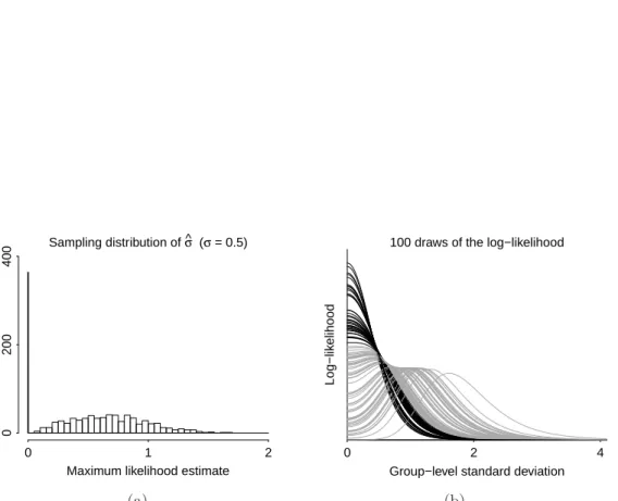
[Figure 1 about here.]
Figure 1(a) shows the sampling distribution of the maximum likelihood estimate of σθ. As
expected, in more than a third of the simulations, the likelihood is maximized at bσθ = 0.
The noise is so much larger than the signal here that it is impossible to do much more than bound the group-level variance; the data do not allow an accurate estimate.
Figure 1b displays 100 draws of the likelihood function, which shows in a different way that the maximum is likely to be on the boundary, with there being quite a bit of uncertainty. We want a point estimator that is positive while being consistent with the data. Setting σθ
to zero would be a mistake, and it would also be wrong to say that the likelihood offers no information at all. In particular, it boundsσθ on the high end. A fair point summary would
be somewhere in the range supported by the likelihood, with a standard error high enough to acknowledge the uncertainty in the inference.
2
Maximum penalized likelihood estimation of
σ
θ2.1 A brief review of the maximum likelihood and restricted maximum likelihood estimation
We consider the model
yij =xTijβ+θj +ǫij, i= 1, . . . , nj, j = 1, . . . , J, J X
j=1
nj =N, (1)
where yij is the response variable and xij is a p-dimensional vector of covariates for unit
i in group j; β is a p-dimensional vector of coefficients that do not vary between groups;
θj ∼ N(0, σθ2) is a group-level error; and ǫij ∼ N(0, σ2ǫ) is a residual for each observation.
We further assume that θj and ǫij are independent.
The parameters (β, σθ, σǫ) are commonly estimated by maximum likelihood (ML).
An-other option is restricted or residualized maximum likelihood (REML, Patterson and Thomp-son, 1971), which is equivalent to specifying uniform priors for the regression coefficients β
and maximizing the marginal posterior mode, integrated overθj andβ (Harville, 1974).
Un-like the ML estimator, the REML estimator of σ2
θ is unbiased in balanced designs (constant
group-size) if it is allowed to be negative.
Discussion of small-sample inference for mixed models has largely focused on the covari-ance matrix of βb (e.g., Kenward and Roger, 1997). Longford (2000) points out that this covariance matrix is often poorly estimated because variance components are estimated in-accurately. The sandwich estimator (Huber, 1967; White, 1990) is asymptotically consistent even if the distributional assumptions are violated. However, as Drum and McCullagh (1993)
note, it can perform poorly when the sample size is small. Crainiceanu et al. (2003) derive a general expression for the probability that the (local) maximum of the marginal (or re-stricted) likelihood is at the boundary for linear mixed models and Crainiceanu and Ruppert (2004) discuss the finite-sample distribution of the likelihood ratio statistic for testing null hypotheses regarding the group-level variance.
2.2 Maximum penalized likelihood estimation
In the present article, we are particularly concerned with the group-level standard deviation, and we specify a penalty or a prior only forσθ, implicitly assuming a uniform prior,p(β, σǫ) =
1, on β and σǫ.
The penalized log-likelihood function can be written as
loglp(σθ,β, σǫ;y) = logl(σθ,β, σǫ;y) + logp(σθ) +c, (2)
where the first term of the right hand side is the log-likelihood, logp(σθ) is an additive penalty
term or log prior, and c is a constant. We find the maximum penalized likelihood (MPL) estimator that attains the maximum of (2). The penalized log-likelihood can be regarded as the marginal log-posterior density with varying intercepts (θj) integrated out and MPL
estimates are equivalent to posterior modal estimates. By integrating the posterior over
θj, we avoid the incidental parameter problem (Neyman and Scott, 1948; O’Hagan, 1976;
Mislevy, 1986).
Unlike posterior mean estimation, posterior modal estimation does not involve simula-tion and is computasimula-tionally as efficient as maximum likelihood estimasimula-tion. In addisimula-tion, by modifying existing maximum likelihood estimation procedures, we can easily find the pos-terior mode. We have implemented maximum penalized likelihood estimation for gllamm
lme4 package (Bates and Maechler, 2010) in R. In both programs, the user has the option to specify a prior and the corresponding log density is added to the log-likelihood during op-timization. (The modifiedgllamm is available from www.gllamm.org and the modifiedlmer
can be found in the blme package available from the Comprehensive R Archive Network.)
2.3 Desired properties of a weakly informative prior
Our goal is to find a penalty or a prior for σθ so that MPL estimates are off the boundary,
but with the penalty being weak enough so that inferences are consistent with the data. For our purpose, we desire p(σθ) that
(i) is zero at the origin and
(ii) has a positive constant derivative at zero.
Condition (i) ensures a positive estimate of the variance parameter, even when the maximum of the likelihood is at 0. Condition (ii) allows the likelihood to dominate if it is strongly curved near zero. The positive constant derivative implies that a prior is linear at zero and there is no “dead zone” in the penalty near zero—that is, the penalty does not rule out positive values near zero if they are supported by the likelihood.
For our default choice of penalty, we do not impose any restriction on the right tail of
p(σθ) since our primary concern is to avoid boundary estimates and the right tail has little
impact on the posterior mode. If the number of groups is small and we want to further control the estimate, it would make sense to assign a finite scale to the prior to constrain the right tail.
Various reasonable-seeming choices of priors do not satisfy both the above conditions. The
exponentialandhalf-Cauchyfamilies, for example, do not decline to zero at the boundary, so they do not rule out posterior mode estimates of zero. Such priors can be excellent weakly
informative priors for full Bayesian (posterior mean) inference (see Gelman, 2006) but do not work if the goal is to get a non-degenerate posterior mode estimate.
The lognormal and inverse-gamma densities satisfy condition (i) but not condition (ii). They have a zero derivative at the origin, essentially ruling out low estimates of σθ no
matter what the data suggest. Thus, the lognormal can only be used when there is real prior information to guide the choices of its two parameters; it cannot be a default choice of the sort we are seeking here.
2.4 Gamma penalty function
We propose the logarithm of a gamma (not inverse-gamma) density as a penalty function of
σθ or equivalently, assign a gamma prior on σθ : defined by
p(σθ) = λα Γ(α)σ α−1 θ e −λσθ, α > 0, λ >0 (3)
with mean α/λand varianceα/λ2
, where αis the shape parameter and λis the rate param-eter (the reciprocal of the scale paramparam-eter).
With an appropriate choice of parameters, the gamma satisfies the two conditions for the weakly informative prior listed in the previous section. For anyα >1, gamma(α, λ) satisfies the first condition that p(0) = 0. In order to have a positive constant derivative at zero (the second condition), α can be chosen to be 2.
We consider three ways to apply the gamma prior as a penalty:
• Our default choice is gamma(α, λ) with α = 2 and λ → 0, which is the (improper) density (p(σθ) ∝ σθ). As we discuss shortly, this default bounds the MPL estimate
away from zero while keeping it consistent with the likelihood.
like to include in our model. Whenα= 2, the gamma density has its mode at 1/λ, and so our recommendation is to use the gamma(α, λ) with 1/λ set to the prior estimate of σθ.
• If strong prior information is available, then both parameters of the gamma density can be set to encode this. If α is given a value higher than 2, property (ii) above will no longer hold, but this is acceptable if this represents real information aboutσθ.
3
Theoretical properties
3.1 Difference between ML estimator and MPL estimator
To examine the effect of α and λ on the MPL estimator analytically, we treat (β, σǫ) as
nuisance parameters and assume that the profile log-likelihood can be approximated by a quadratic function in σθ around the ML estimator, ˆσθML,
logL(σθ)≈ − (σθ−σˆθML) 2 2·se(ˆb σML θ )2 +c1. (4) Herese(ˆb σML
θ ) represents the estimated asymptotic standard error ofσθ(based on the observed
information). This quadratic approximation of the profile log-likelihood function of σθ is
reasonable because the first derivative of the profile log-likelihood (with respect to σθ, not
σ2
θ) at the ML estimate ˆσ
ML
θ is zero even when ˆσ
ML
θ is zero.
For example, consider a balanced varying-intercept model without covariates by setting
xTijβ=µand ni =n in model (1). Then the profile log-likelood of σθ is given by
logLσθ(σθ) =− (n−1)J 2 log ˆσ 2 ǫ − J 2 log ˆ σ2 ǫ +nσ 2 θ − 1 2 SST ˆ σ2 ǫ − nσ2 θ ˆ σ2 ǫ(ˆσǫ2+nσ 2 θ) SSB
where ˆ σ2 ǫ = SSW /(n−1)J if SSB ≥ SSWn−1 SST /nJ if SSB < SSWn−1, SST =PjPi(yij −y¯··)2, SSB =n P j(¯y·j −y¯··)2 and SSW =SST −SSB.
Taking the derivative of logLσθ with respect to σθ, we have
∂logLσθ ∂σθ = − nJ 2(ˆσ2 ǫ +nσ 2 θ) + n·SSB 2(ˆσ2 ǫ +nσ 2 θ)2 ·2σθ. (5)
When we have boundary estimates ofσθ, it is possible that the log-likelihood function of σθ2
has its maximum in the negative region, and so ∂logLσθ/∂(σ
2
θ) (the part in the parenthesis
of the right-hand side in (5)) is negative atσ2
θ = 0. In this case, the quadratic approximation
of logLσθ inσ
2
θ at the boundary will not be appropriate because the linear term still exists.
Even in this case, (5) will be zero because of the factor 2σθ. Therefore, in the Taylor
expansion of logLσθ in σθ at 0, the linear term vanishes, the leading term becomes the
quadratic (with negative coefficient when σbθ = 0) and the higher order terms are negligible
around σθ = 0. In Sections 4 and 5, we will confirm that the quadratic approximation fits
well in an application and in simulations.
Using this quadratic approximation of the profile log-likelihood inσθ, we derive a number
of properties of the log-gamma(α, λ) penalty of σθ. (Derivations are in the supplementary
materials.) In what follows, we discuss the behavior of ˆσθfor two cases: given under Property
1 for ˆσML
θ = 0 and Property 2 for ˆσ
ML
θ >0.
Property 1. When σˆML
θ = 0, for fixedα >1andse(ˆb σ
ML
θ ), the largest possible MPL estimate
is attained when λ→0 with the value
b
σθ =se(ˆb σθML) √
Whenα = 2, we obtainσbθ =se(ˆb σθML). That is, when the ML estimate is on the boundary,
the log-gamma(2, λ) penalty shifts the MPL estimate away from zero but not more than one estimated standard error.
One standard error can be regarded as a statistically insignificant distance from the ML estimate. If the quadratic approximation in (4) holds and ˆσML
θ is zero, the likelihood-ratio
test (LRT) statistic for H0 : σθ = se(ˆb σθML) is 2(logL(0)−logL(se(ˆb σ
ML
θ ))) = 1. For the null
hypothesis σθ = 0, it is known that the asymptotic distribution (as J approaches infinity)
of the test statistic is 0.5χ2
0+ 0.5χ 2
1 with 99th percentile 5.41. In finite samples, the mass at zero is larger and the 99th percentile is smaller, but even with J = 5, the 99th percentile is as large as 3.48, in a model without covariates and large cluster size (Crainiceanu and Ruppert, 2004). For testing H0 : σθ =se(ˆb σθML) (> 0), the percentile will be larger because
there is less point mass at zero (Crainiceanu et al., 2003). Therefore, a LRT statistic of 1 can be considered small.
Property 2. When σˆML
θ >0, for fixedα >1andse(ˆb σ
ML
θ ), the largest possible MPL estimate
is attained when λ→0 with the value
b σθ = ˆ σML θ 2 + ˆ σML θ 2 q 1 + 4(α−1)se(ˆb σML θ ) 2/(ˆσML θ ) 2 >σˆML θ .
In addition, ∂bσθ/∂se(ˆb σMLθ ) decreases in σˆ
ML
θ .
Similar to the case of ˆσML
θ = 0, ˆσθ is greater than ˆσθML and is an increasing function of b
se(ˆσML
θ ). The gradient∂bσθ/∂se(ˆb σMLθ ) has maximum √
α−1 for ˆσML
θ = 0 that coincides with
(6) and decreases as ˆσML
θ increases. This implies that the log-gamma(α, λ) penalty does not
shift the MPL estimate as much when ˆσML
θ >0 as it does when ˆσ
ML
θ = 0 when λ is close to
zero. Therefore it has less influence on the estimate when the ML estimate is plausible than when the ML estimate is on the boundary.
3.2 Asymptotic properties
Although this paper is concerned with the problem of boundary estimates which occur when
J is small, it is important to investigate the asymptotic properties of the proposed estimator as J → ∞ and compare them with the asymptotic properties of the ML estimator.
Consider a balanced varying-intercept model with xT
ijβ = µ and ni = n. For
sim-plicity, we assume that µ and σ2
ǫ are known. Then the ML estimator of σθ is ˆσmlθ = PJ j=1(¯y·j−y¯··) 2 /J−σ2 ǫ/n +1/2 where (·)+ = max(·,0).
When log-gamma(α, λ) penalty is applied to σθ, the MPL estimator, say ˆσθMPL, is a root
of a fifth order polynomial (See the supplementary materials B). Therefore, we do not have a simple formula for ˆσMPL
θ but we can investigate its asymptotic properties using expansions
of the penalized log-likelihood (or the log-posterior) function.
The asymptotic distribution of the ML estimator in linear mixed models is shown in Miller (1977). To examine the asymptotic properties of an estimator forσθ, it is sufficient to assume
only J → ∞ regardless of n. As J → ∞, ˆσML θ is consistent with σ 0 θ and √ J σˆML θ −σ 0 θ follows N(0, I(σ0 θ)− 1 ) asymptotically where I(σ0
θ) is the information matrix and σ
0
θ is the
true value ofσθ.
Fu and Gleser (1975) show that the posterior mode is consistent and has the same limiting distribution as the ML estimator under some regularity conditions that are satisfied for our model. That is, as J → ∞,
√ J(ˆσMPL θ −σ 0 θ)→N 0, I(σ 0 θ)− 1 .
Based on this result, we compare the higher order bias of the ML estimator and the MPL estimator in the following theorem.
Theorem 3. At the order of J−1
fol-lowing bias. E(ˆσML θ ) =σ 0 θ − 1 4(σ0 θ)3J σ2 ǫ n + (σ 0 θ) 2 2 +o(J−1 ) E(ˆσMPL θ ) = σ 0 θ+ α+λσ0 θ −1 2 − 1 4 1 (σ0 θ)3J σ2 ǫ n + (σ 0 θ) 2 2 +o(J−1 )
In addition, with the default prior (α = 2 and λ → 0), two estimators have the same magnitude of bias but negative for σˆML
θ and positive for σˆ
MPL
θ .
Proof. An outline of the proof is in the supplementary materials and Dorie (2012).
The MPL estimator ofσMPL
θ with the default penalty is not only asymptotically unbiased
and as efficient as the ML estimator, but also has the same magnitude of bias at the higher order as seen in Theorem 3. In addition, the MPL estimator tend to be less biased for small
J as will be shown using simulations in Section 5.
3.3 Transformation of σθ
In the Bayesian point of view, when the posterior density ofσθ is asymmetric, a
transforma-tion of σθ can make the density more symmetric so that the posterior mode will be located
near the posterior mean which has good asymptotic properties. Note that while the ML estimator is invariant under transformations, the posterior modal estimator is not due to the change in prior density when transformingσθ. Thus the transformation affects the posterior
mode.
Consider the Box-Cox transformations (Box and Cox, 1964)
gγ(σθ) = σγθ−1 γ if γ 6= 0; log(σθ) if γ = 0 .
equiv-For example, consider a special case with α = 1, λ → 0, and γ = 0, which implies the uniform (improper) prior onσθ and log transformation of σθ. With this prior, the marginal
posterior density is just the likelihood, which is often right-skewed or even has its mode at
σθ = 0 (where the boundary estimation problem occurs). In this case, the log transformation
of σθ can make the shape of the posterior more symmetric. If we maximize the posterior
density of log(σθ), then the maximizer log(dσθ) will be the same as log(ˆσθ) where ˆσθ is the
maximizer of the posterior with gamma(2, λ) prior on σθ.
We have discussed the gamma prior on the group-level standard deviation (σθ) since the
profile log-likelihood as a function of σθ has a better quadratic approximation so it helps us
to investigate the properties in Section 3.1. However, one might still be interested in priors on the variance, σ2
θ.
Property 5. In the limit λ→0, a gamma(α, λ)prior on σ2
θ is equivalent to a gamma(2α−
1, λ) prior on σθ.
Therefore, the properties of the gamma prior in this paper hold for the gamma prior on
σ2
θ with α adjusted appropriately.
3.4 Connection to REML
In Section 2.1, we mentioned that REML gives an unbiased estimate for variance components in the balanced case (when negative variance estimates are permitted). In this section, we regard REML as a penalized likelihood estimator and compare the REML penalty with the log of the gamma density, considered as a penalty on the log-likelihood.
Patterson and Thompson (1971) describes the REML log-likelihood, say logLR, in terms
of the original log-likelihood, L, and an additive penalty term,
logLR= logL−
1
2log det(X
TV−1
whereV is theN×N covariance matrix of the vector of all responses yand X is the design matrix with rows xTij. In the varying-intercept model in (1), V is a block-diagonal matrix with nj ×nj blocks, Vj, j = 1, . . . , J, where Vj contains σθ2 +σ
2
ǫ in the diagonal and σ
2
θ
in the off-diagonals. Recalling that the penalized log-likelihood in (2) is the sum of the log-likelihood and the log-gamma density, the second term in (7), denoted by logpR(σθ), is
analogous to the log of the gamma density function.
In order to compare the REML penalty and log-gamma penalty, we consider a special case of model (1) with balanced group size n, q level-1 covariates, and r level-2 covariates. The level-1 covariates, written as columns z1, . . . ,zq of the design matrix, consist of the
same elements for each group and satisfy 1Tzu = 0, zuTzu′ = 1 if u = u′, and 0 otherwise
for u = 1, . . . , q. The level-2 covariates are assumed to be dummy variables for the first
r(< J −q−2) groups. Then the REML penalty becomes
logpR(σθ) = r+ 1 2 log σ2 θ+ σ2 ǫ n +c1 (8)
where c1 is a constant. The proof is provided in the supplementary materials. Recall that, when λ → 0, the gamma(α, λ) prior on σ2
θ (equivalently gamma(2α−1, λ)
onσθ) has log density,
logp(σ2
θ) = (α−1) logσ
2
θ +c2. (9)
Ignoring the constant terms that have no influence on the posterior mode, we see that the gamma((r+ 1)/2 + 1, λ) on σ2
θ (equivalently gamma(r+ 2, λ) on σθ) approximately matches
the REML penalty, particularly when the group-size n is large and λ is close to zero. The difference between these two penalty terms is clear when σθ is close to zero. At
σθ = 0, the log-gamma penalty term in (9) is −∞ for α > 1, whereas the REML penalty
boundary estimates. Further, it implies that the log-gamma penalty assigns more penalty on
σθ close to zero than REML for small n and largeσǫ. Otherwise, REML can approximately
be viewed as a special case of our method with a log-gamma penalty.
The REML penalty expression in (8) is derived for covariates with specific properties as described above. However, we found that the relationship between the REML and gamma penalty illustrated in this section holds more generally (see the supplementary materials.)
4
Application: meta-analysis of 8-schools data
Alderman and Powers (1980) report the results of randomized experiments of coaching for the Scholastic Aptitude Test (SAT) conducted in eight schools. The data consist of an estimated treatment effect and associated standard error for each school (obtained by separate analyses of the data of each school) and have previously been analyzed by Rubin (1981) and Gelman et al. (2004).
Meta-analysis with varying intercepts (DerSimonian and Laird, 1986), typically called random-effects meta-analysis, allows for heterogeneity among studies due to differences in populations, interventions, and measures of outcomes. The model for the effect size yi of
study i can be written as
yi =µ+θi+ǫi, θi ∼N(0, σθ2), ǫi ∼N(0, s2i), (10)
and allows the effect µ+θi of study i to deviate from the overall effect size µ by a
study-specific amount θi. The estimated effect yi for study i differs from µ+θi by an estimation
error ǫi with standard deviation set equal to the estimated standard error for study i.
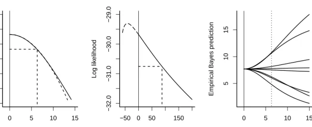
σ2
θ (middle). On the left we see that the profile log-likelihood has its maximum at zero where
the gradient is zero as discussed in Section 3.1. Further, the profile log-likelihood is quite flat. We see in the middle panel of Figure 2 that the profile log-likelihood has a negative gradient at zero as a function of σ2
θ so that the quadratic approximation for σ
2
θ is poor at
the maximum likelihood estimate of zero.
When a researcher is interested in comparing study-specific effects, we can predictθi using
the empirical Bayes predictor, ˜θi =λiyi+ (1−λi)ˆµwhereλi = ˆσθ2/(ˆσ
2
θ+s
2
i) (e.g. Raudenbush
and Bryk, 1985). Whenσθ is estimated as zero, all the studies have the same predicted value
ˆ
µ, The right panel of Figure 2 shows that predictions change rapidly with increasingσθ. The
widths of the empirical Bayes prediction interval also increase with increasing σθ, so that
the uncertainty of the predictions is understated with σθ is underestimated.
Inference forσθis also important because it affects both the point estimate and estimated
standard error of the overall effect size µ,
b se(µb) = " X i 1 s2 i + ˆσ 2 θ #−1/2 . (11)
For example, the estimated standard error is 4.1 for ˆσθ = 0, compared with 5.5 for ˆσθ = 10
(the corresponding estimates of µ are 7.7 and 8.1, respectively.)
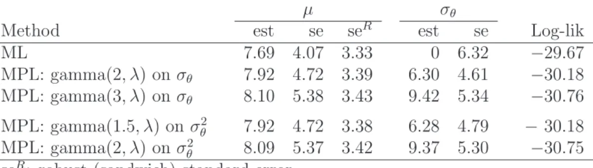
[Table 1 about here.]
For the model in (10), we consider four different penalties: log-gamma(2, λ) and log-gamma(3, λ) on σθ and log-gamma(1.5, λ) and log-gamma(2, λ) on σ2θ, where λ = 10−
4 . MPL estimates with these penalties and ML estimates are given in Table 1. The estimated standard error of ˆσML
θ is 6.32 (which corresponds tose(ˆb σ
ML
θ ) in Section 3.1).
When the penalty is assigned on σθ (rows 2 and 3), ˆσθMPL is 6.30 and 9.42 for α = 2
and α = 3, respectively. These are close to the values se(ˆb σML
)√α−1 with se(ˆb σML
which we expect with ˆσML
θ = 0 if the profile log-likelihood is quadratic in σθ, as it appears
to be in the left panel of Figure 2. In both cases, the log-likelihood at the MPL estimate is only a little bit lower than the maximum log-likelihood.
Specifying a log-gamma(2, λ) penalty on σ2
θ (row 5) gives estimates that agree well with
those for a log-gamma(3, λ) penalty on σθ as expected (see Property 5). Similarly, a
log-gamma(1.5, λ) on σ2
θ (row 4) gives MPL estimates that are close to the estimates with
log-gamma(2, λ) on σθ. A log-gamma penalty on σθ2 with α = 1.5 corresponds to REML
with no level-2 covariates. While REML givesσbθ = 0 (not shown here), a log-gamma penalty
with α= 1.5 gives a legitimate estimate and decreases the log-likelihood by only 0.5. Table 1 also reports model-based and robust standard error estimates for µb (seR). We
see that the estimated model-based standard error of the estimated overall effect size µ
increases with σθ as implied by (11), whereas the robust standard errors, based on the
sandwich estimator, change very little.
5
Simulation study: balanced varying-intercept model
We consider a varying-intercept model,
yij =β0+θj +β1x1ij +β2x2ij +ǫij, i= 1, . . . , n, j= 1, . . . , J (12)
with J = 3,5,10,30 groups and n = 5,30 observations per group. This model includes two covariates: x1ij = i varies within groups only (its mean is constant across groups),
and x2ij = j varies between groups only. The coefficients β0, β1, β2 are fixed parameters,
θj ∼ N(0, σθ2) is a varying intercept for each group, and ǫij ∼ N(0, σǫ2) is an error for each
observation.
β0 = 0, β1 =β2 = 1, σǫ = 1, and σθ = 0,1/ √
3, or 1, which correspond to intra-class corre-lations ρ = 0,0.25 and 0.5, respectively. Although our method is based on the assumption that σθ > 0, we include the condition σθ = 0 as the worst-case scenario. We obtain MPL
estimates with log-gamma(2, λ) and log-gamma(3,λ) penalties on σθ, where λ= 10−4. The
REML penalty corresponds toα= 3 since the model contains one group-level covariate. We compare MPL estimates with ML and REML estimates.
Boundary estimates Here we report the proportion of estimates of σθ that are on the
boundary (less than 10−5
) when the true σθ is not zero (1/ √
3 and 1). For σθ = 1/ √
3, 47% of ML estimates and 45% of REML estimates are zero for J = 3 and n = 5. As J or n
increases, the proportion decreases, but for J = 5 and n = 30, the proportion of estimates on the boundary is still 5% for ML and 4% for REML.
When σθ = 1, the same pattern occurs but estimates are on the boundary less often for
a given condition. For J = 3 and n = 5, ML produces 34% of estimates on the boundary compared with 32% for REML. When J increases to 5 and n to 30, 1% of ML estimates and 0.7% of REML estimates are on the boundary. When J = 30, ML and REML yield no boundary estimates for either value of σθ.
In contrast to the ML and REML estimates, the MPL estimates are never on the bound-ary in any of the simulation conditions. At the same time, the likelihood at the MPL estimates does not differ considerably from the maximum. The likelihood ratio test statistic
−2logL(bσMPL
θ )−logL(σb
ML
θ )
for testing the restriction σθ =bσθMPL was calculated for each
replicate. When J > 3, the largest test statistic among all the replicates and simulation conditions is 2.60. Even for J = 3, the largest test statistic is 3.45. As discussed in Section 3.2, these values are not large.
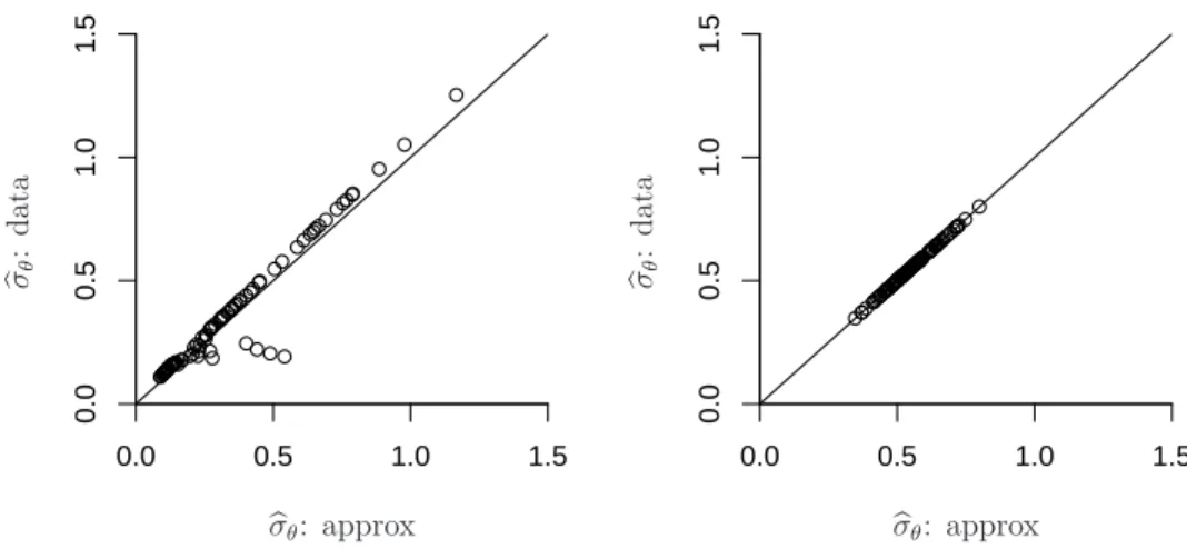
Quadratic approximation
[Figure 3 about here.]
We now assess how well some of the relationships hold that were derived in Section 3.1 by assuming that the profile log-likelihood is quadratic. Figure 3 shows that the MPL estimates calculated by the quadratic approximation of the profile log-likelihood (see properties 1 and 2) agree well with the MPL estimates with a log-gamma(2,λ) penalty onσθ for J = 3 (left)
and J = 30 (right) when ρ= 0.25 andn = 30.
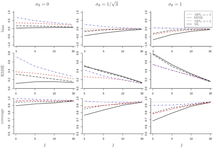
[Figure 4 about here.]
Figure 4 summarizes the estimated bias and the root mean squared error (RMSE) of σθ,
and the coverage of 95% confidence intervals (CI) for β2 for the four methods for n = 5,
J = 3,5,10,30 and σθ = 0,1/ √
3,1. Results for n = 30 are given in the supplementary materials.
Estimates of σˆθ The first row of Figure 4 shows that the bias for σθ decreases as J
increases and σθ decreases. Thus the differences between methods are most obvious with
small J, and particularly when σθ >0.
For σθ > 0, both REML and ML tend to underestimate σθ. MPL estimates with a
log-gamma(2, λ) penalty also tend to be downward biased for σθ but not as much as the
ML estimates. On the other hand, the MPL estimator with log-gamma(3, λ) produces the largest estimates among the four estimators so it often overestimates σθ. For σθ = 1, the
MPL estimator with log-gamma(3, λ) has the smallest bias for all J.
When σθ = 0, as expected, the MPL estimators assign more penalty on the values close
to the boundary than REML, so the bias is larger than for REML and ML.
confirms that the log-gamma penalty on σθ with α = 3 agrees with the REML penalty
when the model contains one group-level covariate, particularly with largen, as discussed in Section 3.4.
The root mean squared errors (RMSE) of both MPL estimators are consistently smaller than for ML and REML when σθ is not zero (see second row of the figure). For σθ = 1/
√
3 and σθ = 1, REML has smaller bias than MPL with log-gamma(2, λ) but its RMSE is
significantly larger because the REML estimates have the largest variance among the four estimators. The MPL estimator tends to have smaller RMSE with log-gamma(2, λ) than with log-gamma(3, λ) but the difference decreases as n,J and σθ increase.
Coverage of CI for β2 The standard error estimates of the estimated coefficient of the
group-level covariate (βb2) is greatly influenced by bσθ. The squared asymptotic standard
error ofβb2 from the Hessian matrix is Var(βb2)≈(nσ2θ +σǫ2)/nJs2X
2 wheresX2 is the standard
deviation of the group-level covariateX2(Snijders and Bosker, 1993). When the true variance is not zero but bσθ is on the boundary, the standard error of βb2 will be underestimated and the CI will be too narrow.
The third row of Figure 4 shows the proportions of 95% CI that cover the true value of
β2. The gray solid line shows the nominal coverage (0.95). For all values of σθ, ML gives CI with lower than nominal coverage. For σθ = 0, all the methods except ML tend to have
higher than nominal coverage.
When σθ > 0, most of the methods have lower than nominal coverage, but the MPL
estimator with α= 3 has the best coverage, particularly forσθ = 1/ √
3. Although the MPL estimator with α = 3 tends to have large positive bias for σθ, it turns out to give better
coverage. Recalling that log-gamma(3, λ) is close to the REML penalty (discussed in Section 3.4) for large n, we found that the coverage for the MPL estimator with α = 3 is closer to REML forn= 30 (not shown here) than for n= 5. However, REML still shows significantly
lower coverage than the MPL estimator, particularly for smallJ.
In summary, the MPL estimator with a log-gamma penalty is successful at avoiding boundary solutions and, at the same time, the likelihood does not change substantially most of the time. Furthermore, the MPL method performs as well as or better than ML or REML: if σθ is not zero, RMSE of bσθ is uniformly lower for the MPL estimator with both
log-gamma penalties than for REML and the ML estimator and coverage of the CI for the fixed coefficient for the group-level covariate is best for the MPL estimator with α = 3. Although there is no obvious winner between gamma withα = 2 andα= 3, neither penalty ever produces a boundary estimate (bσθ <10−5).
We also performed a simulation study for unbalanced variance component models without any covariates, following Swallow and Monahan (1984). For two different unbalanced pat-terns withσθ = 0,1/
√
3,1, we compared ML and REML estimates with MPL estimates with a gamma(2,λ) prior, which corresponds to the REML penalty when there is no group-level covariate. (Results are in the supplementary materials.)
Similar to the balanced case, when σθ is not zero, ML and REML tend to underestimate
σθ and the RMSE tends to be larger than for the MPL estimates. The advantage of the
gamma prior in terms of the RMSE is more obvious for σθ = 1. The standard errors of
the fixed intercept estimate are also underestimated by ML and REML when σθ is not zero
while the MPL estimators perform better in this regard.
6
Discussion
In this paper, we considered linear varying-intercept models and suggested specifying a log-gamma penalty for the group-level standard deviation to avoid boundary estimates. We showed that our procedure guarantees non-zero estimates of the group-level variance, while maintaining statistical properties as good or better than maximum likelihood and restricted
maximum likelihood when the true group-level variance is not too close to zero. The penalty (or prior) is only weakly informative in the sense that the log-likelihood at the maximum penalized likelihood estimates tends to be not much lower than the maximum.
We have shown that this strategy of accepting the maximum likelihood estimate results in under-coverage of confidence intervals for regression coefficients of group-level covariates. In datasets where boundary estimates occur, a large range of values of the group-level standard deviation is often supported by the data, and our method provides one such value. Our approach is hence somewhere between purely data-based maximum likelihood estimation and setting the variance to a constant instead of estimating it, as suggested by Longford (2000) for the purpose of obtaining better standard errors and by Greenland (2000) when the variance is not identified.
Our idea can also be applied to models with varying intercepts and slopes where the problem is to regularize the covariance matrix, say Σ, away from its boundary, |Σ| = 0. In this case, the gamma prior can be naturally extended to the Wishart prior on Σ, which is equivalent to the product of gamma priors on the eigenvalues of Σ1/2
. Therefore the Wishart prior with a certain choice of parameters will shift the posterior mode of each eigenvalue away from 0, or equivalently move the posterior mode of Σ away from the singularity. At the same time, it moves the eigenvalues approximately at most one standard error away from the ML estimates as did the gamma(2,λ) in the univariate case.
Other applications of our approach include generalized linear mixed models, models with more hierarchical levels, and latent variable models of all sorts—basically, any models in which there are variance parameters that could be estimated at zero.
Another generalization arises when there are many variance parameters—either from a large group-level covariance matrix, several different levels of variation in a multilevel model, or both. In any of these settings, it can make sense to stabilize the estimated variance parameters by modeling them together, adding another level of the hierarchy to
allow partial pooling of estimated variances.
Finally, from a computational as well as an inferential perspective, a natural interpreta-tion of a posterior mode is as a starting point for full Bayes inference, in which informative priors are specified for all parameters in the model and Metropolis or Gibbs jumping is used to capture uncertainty in the coefficients and the variance parameters (Dorie et al., 2011). For reasons discussed above, it can make sense to switch to a different class of priors when moving to full Bayes: once modal estimation is abandoned, there is no general reason to work with priors that go to zero at the boundary.
Supporting Information
A supplementary material contains derivation of properties in Section 3, proofs of Theorem 3 and equation (7), REML and gamma priors in general cases, and additional simulation results.
References
Alderman, D. and Powers, D. “The effects of special preparation on SAT-Verbal scores.”
American Educational Research Journal, 17(2):239–251 (1980).
Bates, D. and Maechler, M. lme4: linear mixed-effects models using S4 classes (2010). R package version 0.999375-37.
URLhttp://CRAN.R-project.org/package=lme4
Box, G. and Cox, D. “An analysis of transformations.” Journal of the Royal Statistical Society. Series B (Methodological), 26(2):211–252 (1964).
Crainiceanu, C. and Ruppert, D. “Likelihood ratio tests in linear mixed models with one vari-ance component.” Journal of the Royal Statistical Society: Series B (Statistical Method-ology), 66(1):165–185 (2004).
Crainiceanu, C., Ruppert, D., and Vogelsang, T. “Some properties of like-lihood ratio tests in linear mixed models.” Technical report, available at http://www.orie.cornell.edu/∼davidr/papers (2003).
Curcio, D. and Verde, P. “Comment on: Efficacy and safety of tigecycline: a systematic review and meta-analysis.” Journal of Antimicrobial Chemotherapy Advanced Access, doi: 10.1093/jac/dkr353 (2011).
DerSimonian, R. and Laird, N. “Meta-analysis in clinical trials.” Controlled Clinical Trials, 7:177–188 (1986).
Dorie, V. “Mixed Methods for Mixed Models: Bayesian Point Estimation and Classical Uncertainty Measures in Multilevel Models.” Ph.D. thesis, Columbia University (2012). Dorie, V., Liu, J., and Gelman, A. “Bridging between point estimation and Bayesian
infer-ence for generalized linear models.” Technical report, Department of Statistics, Columbia University (2011).
Draper, D. “Assessment and propagation of model uncertainty.” Journal of the Royal Statistical Society. Series B (Methodological), 57(1):45–97 (1995).
Drum, M. and McCullagh, P. “[Regression models for discrete longitudinal responses]: Com-ment.” Statistical Science, 8(3):300–301 (1993).
Fu, J. and Gleser, L. “Classical asymptotic properties of a certain estimator related to the maximum likelihood estimator.” Annals of the Institute of Statistical Mathematics, 27(1):213–233 (1975).
Galindo-Garre, F. and Vermunt, J. “Avoiding boundary estimates in latent class analysis by Bayesian posterior mode estimation.” Behaviormetrika, 33(1):43–59 (2006).
Galindo-Garre, F., Vermunt, J., and Bergsma, W. “Bayesian posterior mode estimation of logit parameters with small samples.” Sociological Methods & Research, 33(1):88–117 (2004).
Gelman, A. “Prior distributions for variance parameters in hierarchical models.” Bayesian Analysis, 1(3):515–533 (2006).
Gelman, A., Carlin, J., Stern, H., and Rubin, D. Bayesian Data Analysis, second edition. Champan and Hall/CRC (2004).
Gelman, A. and Meng, X. “Model checking and model improvement.” In Markov Chain Monte Carlo in Practice, 189–201. Chapman and Hall (1996).
Gelman, A., Shor, B., Bafumi, J., and Park, D. “Rich state, poor state, red state, blue state: What′s the matter with Connecticut?” Quarterly Journal of Political Science,
2(4):345–367 (2007).
Greenland, S. “When should epidemiologic regressions use random coefficients?” Biometrics, 56(3):915–921 (2000).
Hardy, R. and Thompson, S. “Detecting and describing heterogeneity in meta-analysis.”
Harville, D. A. “Bayesian inference for variance components using only error contrasts.”
Biometrika, 61(2):383–385 (1974).
—. “Maximum likelihood approaches to variance components estimation and related prob-lems.” Journal of the American Statistical Association, 72:320–340 (1977).
Huber, P. J. “The behavior of maximum likelihood estimation under nonstandard condition.” In LeCam, L. M. and Neyman., J. (eds.),Proceedings of the Fifth Berkeley Symposium on Mathematical Statistics and Probability 1, 221–233. University of California Press (1967). Kelly, R. and Mathew, T. “Improved nonnegative estimation of variance components in
some mixed models with unbalanced data.” Technometrics, 171–181 (1994).
Kenward, M. and Roger, J. H. “Small-sample inference for fixed effects from restricted maximum likelihood.” Biometrics, 53(3):983–997 (1997).
Kubokawa, T. and Tsai, M. “Estimation of covariance matrices in fixed and mixed effects linear models.” Journal of Multivariate Analysis, 97(10):2242–2261 (2006).
Laird, N. M. and Ware, J. H. “Random effects models for longitudinal data.” Biometrics, 38:963–974 (1982).
Longford, N. T. “On estimating standard errors in multilevel analysis.” Journal of the Royal Statistical Society: Series D (The Statistician), 49(3):389–398 (2000).
Maris, E. “Estimating multiple classification latent class models.” Psychometrika, 64(2):187– 212 (1999).
Mathew, T. and Niyogi, A. “Improved nonnegative estimation of variance components in balanced multivariate mixed models.” Journal of Multivariate Analysis (1994).
Miller, J. “Asymptotic properties of maximum likelihood estimates in the mixed model of the analysis of variance.” The Annals of Statistics, 5(4):746–762 (1977).
Mislevy, R. J. “Bayes modal estimation in item response models.” Psychometrika, 51(2):177– 195 (1986).
Neyman, J. and Scott, E. L. “Consistent estimates based on partially consistent observa-tions.” Econometrica, 16(1):1–32 (1948).
O’Hagan, A. “On posterior joint and marginal modes.” Biometrika, 63(2):329–333 (1976). Patterson, H. D. and Thompson, R. “Recovery of inter-block information when block sizes
are unequal.” Biometrika, 58(3):545–554 (1971).
Rabe-Hesketh, S. and Skrondal, A. Multilevel and Longitudinal Modeling Using Stata, second ed.. Stata Press (2008).
Rabe-Hesketh, S., Skrondal, A., and Pickles, A. “Maximum likelihood estimation of limited and discrete dependent variable models with nested random effects.” Journal of Econo-metrics, 128:301–323 (2005).
Raudenbush, S. and Bryk, A. “Empirical Bayes meta-analysis.” Journal of Educational and Behavioral Statistics, 10(2):75 (1985).
Rubin, D. B. “Estimation in parallel randomized experiments.” Journal of Educational Statistics, 6(4):377–401 (1981).
Snijders, T. and Bosker, R. “Standard errors and sample sizes for two-level research.” Journal of Educational and Behavioral Statistics, 18(3):237–259 (1993).
Srivastava, M. and Kubokawa, T. “Improved nonnegative estimation of multivariate com-ponents of variance.” Annals of Statistics, 2008–2032 (1999).
Swallow, W. and Monahan, J. “Monte Carlo comparison of ANOVA, MIVQUE, REML, and ML estimators of variance components.” Technometrics, 26(1):47–57 (1984).
Swaminathan, H. and Gifford, J. A. “Bayesian estimation in the two-parameter logistic model.” Psychometrika, 50(3):349–364 (1985).
Tsutakawa, R. K. and Lin, H. Y. “Bayesian estimation of item response curves.” Psychome-trika, 51(2):251–267 (1986).
Verbeke, G. and Molenberghs, G. Linear Mixed Models for Longitudinal Data. Springer Verlag (2000).
White, H. “A heteroscedasticity-consistent covariance matrix estimator and a direct test for heteroscedasticity.” Econometrica, 48:817–838 (1990).
Yeojin Chung, Graduate School of Education, University of California, Berkeley, 4623 Tol-man Hall, Berkeley, CA 94720
Maximum likelihood estimate
Frequency (out of 1000 sim
ulations) 0 1 2 0 200 400 Sampling distribution of σ^ (σ = 0.5) (a)
Group−level standard deviation
0 2 4
Log−lik
elihood
100 draws of the log−likelihood
(b)
Figure 1: From a simple one-dimensional hierarchical model with scale parameter 0.5 and data in 10 groups: (a) Sampling distribution of the maximum likelihood estimate bσθ, based
on 1000 simulations of data from the model. (b) 100 simulations of the log-likelihood. The dark lines are the log-likelihoods with maximum at 0 and the grey lines are the others. The maximum likelihood estimate is extremely variable and the likelihood function is not very informative about σθ.
0 5 10 15 −32.0 −31.0 −30.0 −29.0 Standard deviation Log lik elihood −50 0 50 150 −32.0 −31.0 −30.0 −29.0 Variance Log lik elihood 0 5 10 15 5 10 15 Standard deviation Empir ical Ba y es prediction
Figure 2: Profile log-likelihood as a function of σθ (left) and σ2θ (middle) and empirical
Bayes prediction (right) for 8-schools data. The dashed curve on the left is the quadratic approximation at the mode, based on the estimated standard error. The vertical dashed line is the MPL estimate for a log-gamma(2,λ) penalty on σθ (left) or σθ2 (middle). The vertical
dotted line on the right panel indicates one standard error of σˆML
0.0 0.5 1.0 1.5 0.0 0.5 1.0 1.5 0.0 0.5 1.0 1.5 0.0 0.5 1.0 1.5 b σθ : d at a b σθ : d at a b σθ: approx b σθ: approx
Figure 3: MPL estimates with log-gamma(2,λ) penalty on σθ for J = 3 (left) and J = 30
(right), ρ = 0.25 and n = 30 for the first 100 replicates, compared with the MPL estimates based on the quadratic approximation of the profile log-likelihood (see properties 1 and 2). Agreement is good, suggesting that the quadratic approximation is good. Dots on the left graph that fall off the line are due to a few samples that have uncommonly large estimated standard errors.
σθ = 0 σθ= 1/ √ 3 σθ= 1 3 5 10 30 −1.0 −0.5 0.0 0.5 1.0 b ia s 3 5 10 30 −1.0 −0.5 0.0 0.5 1.0 3 5 10 30 −1.0 −0.5 0.0 0.5 1.0 MPL:α= 3 MPL:α= 2 REML ML 3 5 10 30 0.0 0.2 0.4 0.6 0.8 R M S E 3 5 10 30 0.0 0.2 0.4 0.6 0.8 3 5 10 30 0.0 0.2 0.4 0.6 0.8 3 5 10 30 0.5 0.6 0.7 0.8 0.9 1.0 J co ve ra ge 3 5 10 30 0.5 0.6 0.7 0.8 0.9 1.0 J 3 5 10 30 0.5 0.6 0.7 0.8 0.9 1.0 J
Figure 4: Bias of σθ , RMSE of σθ and coverage of CI for β2 for group size 5, standard
deviation σθ = 0,1/ √
3, and 1 (columns) and number of groups J = 3,5,10,30 (x-axis). Different estimators are represented by different line patterns. Whenσθ >0, all the methods
outperform ML. Bias of the MPL estimator is as low as REML depending on α. RMSE of the MPL estimator with both α is smaller than REML and ML. Coverage of CI is best for the MPL estimator with α = 3.
Table 1: ML and MPL estimates for the 8 schools data, where the penalty is log-gamma(α, λ) on σθ or σ2θ, with λ = 10−
4
. With log-gamma(α, λ) penalty on σθ, the MPL estimates
are approximately at se(ˆb σML
θ )
√
1−α and agree well with the MPL estimates with log-gamma((α+ 1)/2, λ) onσ2
θ.
µ σθ
Method est se seR est se Log-lik
ML 7.69 4.07 3.33 0 6.32 −29.67 MPL: gamma(2, λ) on σθ 7.92 4.72 3.39 6.30 4.61 −30.18 MPL: gamma(3, λ) on σθ 8.10 5.38 3.43 9.42 5.34 −30.76 MPL: gamma(1.5, λ) on σ2 θ 7.92 4.72 3.38 6.28 4.79 −30.18 MPL: gamma(2, λ) on σ2 θ 8.09 5.37 3.42 9.37 5.30 −30.75