arXiv:quant-ph/0602129v1 15 Feb 2006
Non-catastrophic Encoders and Encoder Inverses for
Quantum Convolutional Codes
Markus Grassl
Institut f¨ur Algorithmen und Kognitive Systeme Fakult¨at f¨ur Informatik, Universit¨at Karlsruhe (TH)
Am Fasanengarten 5, 76128 Karlsruhe, Germany Email: [email protected]
Martin R¨otteler
NEC Laboratories America, Inc. 4 Independence Way, Suite 200
Princeton, NJ 08540, U.S.A. Email: [email protected]
Abstract— We present an algorithm to construct quantum
circuits for encoding and inverse encoding of quantum convo-lutional codes. We show that any quantum convoconvo-lutional code contains a subcode of finite index which has a non-catastrophic encoding circuit. Our work generalizes the conditions for non-catastrophic encoders derived in a paper by Ollivier and Tillich (quant-ph/0401134) which are applicable only for a restricted class of quantum convolutional codes. We also show that the encoders and their inverses constructed by our method naturally can be applied online, i. e., qubits can be sent and received with constant delay.
I. INTRODUCTION
Similar to the classical case a quantum convolutional code encodes an incoming stream of quantum information into an outgoing stream. A theory of quantum convolutional codes based on infinite stabilizer matrices has been developed re-cently, see [12]. While some constructions of quantum con-volutional codes are known, see [2], [3], [1], [5], [6], [7], [11], [12], some very basic questions about the structure of quantum convolutional codes and their encoding circuits have not been addressed so far, respectively have been addressed only in special cases. In this paper we focus on the question of which quantum convolutional codes have non-catastrophic encoders, respectively inverse encoders.
Recall, that classically a code encoded by a catastrophic encoder has the unwanted property that—after code word estimation—a finite number of error locations can be mapped by the inverse encoder to an infinite number of error locations. For classical convolutional codes it is well-known that the non-catastrophicity condition is a property of the encoder and not of the code itself. Indeed, every convolutional code has both catastrophic and non-catastrophic encoders and therefore the choice of a good encoder is very important.
In this paper we address the analogous question whether any quantum convolutional stabilizer code has non-catastrophic encoders and encoder inverses. Here the condition to be non-catastrophic has been shown in [12] to be that it has a constant depth encoder whose elementary quantum gates can be ar-ranged in form of a “pearl necklace”, i. e., a regular structure in which blocks are only allowed to overlap with their neighbors with possibly some blocks spaced out. Furthermore, in [12] some conditions on the code have been given under which a non-catastrophic encoder exists. However, these conditions
are quite strict and not applicable to an arbitrary quantum convolutional code.
Using the matrix description of quantum convolutional stabilizer codes and transformations on this matrix which preserve the symplectic orthogonality, we show that a normal form can be achieved which corresponds to a very simple convolutional code. Reducing the dimension of this code by only a bounded factor, we obtain an even simpler code allowing online encoding and decoding. Furthermore, from the sequence of transformations one can read off a non-catastrophic encoder for a subcode of the original code whose dimension is reduced by the same factor. Asymptotically, the rate of the subcode and the original code are the same.
II. QUANTUMCONVOLUTIONALCODES
Quantum convolutional codes are defined as infinite versions of quantum stabilizer codes. We briefly recall the necessary definitions and the polynomial formalism to describe quantum convolutional codes which was introduced in [12].
Definition 1 (Infinite Pauli Group): Let
X= 0 1 1 0 , Z= 1 0 0 −1 , Y=XZ= 0 −1 1 0
be the (real version of the)2×2 Pauli matrices. Consider an infinite set of qubits labeled by the nonnegative integers N. LetM ∈ {X, Y, Z}be a Pauli matrix. We denote byMi the semi-infinite tensor productI2⊗. . .⊗I2⊗M⊗I2⊗. . ., where
M operates on qubit i andI2 denotes the identity matrix of
size 2×2. The group generated by all Xi and Zi fori∈N is called the infinite Pauli group P∞. For an element A =
A1⊗A2⊗. . . ∈ P∞ the positions in which Ai is not equal to±I2 is called the support ofA.
In the theory of block stabilizer codes, the elements of the Pauli group are labeled by tuples of binary vectors. Similarly, we can label the elements of the infinite Pauli group by a tuple of binary sequences, each of which is represented by a formal power series. Hence we get the correspondence
(−1)cXαZβ := (−1)cO ℓ≥0 XαℓZβℓ ˆ = X ℓ≥0 αℓDℓ,X ℓ≥0 βℓDℓ
wherec∈F2 andα=P
ℓ≥0αℓD
ℓ andβ=P ℓ≥0βℓD
ℓ are
formal power series with coefficients inF2. In this representa-tion, multiplication of elements ofP∞corresponds to addition of the power series. Furthermore, shifting an elementA∈ P∞ one qubit to the right corresponds to the multiplication of the power series by D. As we also allow to shift the operators by a bounded number of qubits to the left, we use Laurent series instead of power series to represent the elements of
P∞. An elementA∈ P∞with finite support corresponds to a tuple of Laurent polynomials. Recall that the field of Laurent series in the variableD with coefficients inF2 is denoted by F2((D))and recall further that it contains the ringF2[D, D−1] of Laurent polynomials.
We are interested in shift invariant abelian subgroups ofP∞, more specifically in those subgroups which can be generated by a finite number of elements and their shifted versions. The following definition introduces a shorthand notation for describing such subgroups.
Definition 2 (Stabilizer Matrix): Let S be an abelian sub-group of P∞ which has trivial intersection with the cen-ter of P∞. Furthermore, let {g1, g2, . . . , gr} where gi =
(−1)ciXα
iZβi with ci ∈ {0,1} and (αi,βi)∈F2((D))
n×
F2((D))n be a minimal set of generators for S. Then a stabilizer matrix of the corresponding quantum convolutional (stabilizer) code C is a generator matrix of the (classical) additive convolutional code C ⊆ F2((D))n × F2((D))n generated by (αi,βi). We will write this matrix in the form
S(D) = (X(D)|Z(D)) = α1 β1 .. . ... αr βr ∈F2((D)) r×2n. (1) In what follows we are only interested in those stabilizers which have a finite description. Hence we will consider only such stabilizer matrices (1) in which all entries are actually rational functions, i. e., elements of F2(D). Eventually, we will require that all entries have finite support and are hence polynomials.
Alternatively to (1) a quantum convolutional code can also be described in terms of a semi-infinite stabilizer matrix S
which has entries in F2 ×F2. The general structure of the matrix is as follows: S := G0 G1 . . . Gm 0 . . . 0 G0 G1 . . . Gm 0 . . . 0 0 G0 G1 . . . Gm 0 . . . .. . . .. . .. . .. (2)
The matrix S has a block band structure where each block is of size (n−k)×(m+ 1)n. All blocks have equal size and are comprised of m+ 1matricesG0, G1, . . . , Gm which are
of size (n−k)×n each. In the second block, these m+ 1 matrices are shifted byncolumns, hence any two consecutive blocks overlap in (m−1)npositions.
Similar to the classical case the link between the polynomial description of eq. (1) and the semi-infinite matrix eq. (2) is given byS(D) :=Pm
i=0GiDi. The band structure of eq. (2)
implies that for every qubit in the semi-infinite stream of qubits, there is a bounded number of generators of the stabi-lizer group that act non-trivially on that position. Moreover, as these generators of the stabilizer group have bounded support, their eigenvalues can be measured when the corresponding qubits have been received. Therefore, it is possible to compute the error syndrome for the quantum convolutional code online. Writing the stabilizer in the formS(D) = (X(D)|Z(D))as in eq. (1), it was shown in [12] that the condition of symplectic orthogonality of the semi-infinite matrixS can be expressed compactly in the form
X(D)Z(1/D)t+Z(D)X(1/D)t= 0. (3)
On the other hand, we can start with an arbitrary self-orthogonal additive convolutional code over F2((D))n × F2((D))nto define a convolutional quantum code. In general, the generator matrix for such a code may contain rational functions, but there is always an equivalent description in terms of a matrix with polynomial entries [9]. The following theorem shows that for self-dual convolutional codes, all entries of a systematic generator matrix are in fact Laurent polynomials.
Theorem 3: Let S(D) = (X(D)|Z(D)) with X(D) = I
be a stabilizer matrix of a self-dual additive convolutional code over the rational function fieldF2(D). ThenZ(1/D) =
Z(D)tand all entries ofZ(D)are Laurent polynomials.
Proof: From condition (3) it follows that the code is self-dual if and only if Z(1/D) = Z(D)t. Assume that Zij(D) is a proper rational function and not a Laurent poly-nomial. Then evaluating the series expansion of Zij(D) at 1/D yields infinitely many negative powers. However, since
Zji(D)contains only finitely many negative powers we get a contradiction. Hence all entries ofZ(D) have to be Laurent polynomials.
The symmetryZ(1/D) =Z(D)t additionally implies that
the diagonal termsZii(D)are Laurent polynomials of the form
Zii(D) =
d X
ℓ=0
cℓ(D−ℓ+Dℓ). (4)
III. SHIFT-INVARIANT CLIFFORDOPERATIONS We are interested in quantum circuits which encode a convo-lutional quantum code. Recall that the controlled-not (CNOT) maps|xi|yi 7→ |xi|x⊕yiand that the controlled-Z (CSIGN) gates maps |xi|yi 7→(−1)x·y|xi|yi (see [10]). We want that
errors which happen during the encoding do not be spread out too far. A particularly bad example of spreading errors is given by the cascade CNOT∞ = Q∞
i=0CNOT (i,i+1)
where gates with smaller index i are applied first. The cascadeCNOT∞ maps the finite support elementX⊗I2⊗I2⊗. . .to the infinite
support elementX⊗X⊗X⊗. . .On the other hand the infinite cascadeCSIGN∞ =Q∞
i=0CSIGN
(i,i+1) does not have this
behavior: indeed, a Pauli matrixXiis mapped toZi−1XiZi+1
operators, this shows that it maps finite support Pauli matrices to finite support Pauli matrices. The reason for this difference is that the sequence CSIGN∞ can be parallelized to have finite depth (actually depth2), whereas this is not possible for CNOT∞. Clearly, any circuit of constant depth only leads to a local error expansion, i. e., Pauli matrices with finite support get mapped onto Pauli matrices with finite support. This gives rise to the following definition:
Definition 4 (Non-catastrophic encoder): Let C be a quan-tum convolutional code and let E be an encoding circuit for
C. ThenE is called non-catastrophic if the gates inE can be arranged into a circuit of finite depth.
In the following, we consider infinite cascades of gates from the Clifford group that can be realized by quantum circuits with constant depth. Since the generators for the quantum convolutional code are obtained by shifting a fixed block an infinite number of times, we have to impose a shift invariance condition on any Clifford gate that we intend to apply to the code. This means that whenever a gate is applied it has to be applied also in a shifted version by an offset of n qubits. Similar to the approach in [8], the action of such operations on elements of the infinite Pauli group can be described as linear transformations on the stabilizer matrix. As an example, the action of an infinitely replicated Hadamard gate H on a qubit is described in its action on the vectors(f(D), g(D))∈
F2(D)2 by the matrix H = 0 1 1 0 since H†XH = Z and H†ZH =X. Similarly, all infinitely replicated versions of Clifford gates which only operate within a block and do not connect qubits between shifted blocks, correspond to the usual matrices in the symplectic groupSp2n(F2).
More interesting are those operations which connect differ-ent blocks which have been shifted in time. An example is a CNOT gate which operates on a qubit i (control) and qubit
j (target), where qubitj has been shifted byℓ blocks. Recall that shifting by ℓ blocks corresponds to multiplying by Dℓ.
In this case we obtain that CNOT gate maps the stabilizer vector(x1, x2|z1, z2)7→(x1, x2+x1Dℓ|z1+z2D−ℓ, z2), i. e.,
X errors are propagated into the future andZ errors into the past. Note that by applying a sequence of CNOT gates we can actually map (x1, x2|z1, z2) 7→ (x1, x2+f(D)x1|z1+
f(1/D)z2, z2), where f(D)∈F2[D] is an arbitrary
polyno-mial. A summary of the gates used is shown in Table I. It is important to note that all the operations shown in Table I can be parallelized to have constant depth.
IV. COMPUTING ANENCODINGCIRCUIT
In the following we describe an algorithm which operate on the stabilizer matrix (1) in order to produce a new stabilizer which is in a simpler form. We can act in two ways: (i) by applying row operations using an invertible matrix over F2[D, D−1]. Apart from possible shifts, this does not change
the stabilizer group, i. e., up to a possibly new initial qubit sequence (of bounded length) the quantum code is unchanged. We can also apply (ii) column operations given by an arbitrary element of the Clifford group shown in Table I. Before we state
TABLE I
ACTION OF VARIOUSCLIFFORD OPERATIONS.
unitary gateU matrixU
H= √1 2 1 1 1 −1 ∈C2 ×2 H= 0 1 1 0 ∈F2 ×2 2 P= 1 0 0 exp(iπ/2) ∈C2 ×2 P = 1 1 0 1 ∈F2 ×2 2
CNOT(i,j+ℓn), i6≡j (modn) CNOT =
1 Dℓ 0 0 0 1 0 0 0 0 1 0 0 0 D−ℓ 1
CSIGN(i,j+ℓn), i6≡j (modn) CSIGN=
1 0 0 Dℓ 0 1 D−ℓ 0 0 0 1 0 0 0 0 1 Pℓ:=CSIGN(i,i+ℓn), ℓ6= 0 Pℓ= 1 D−ℓ+Dℓ 0 1
Conjugation of the stabilizer groupS by the unitary gateU corresponds to the action of the matricesUon the columns of the stabilizer matrixS(D) = (X(D)|Z(D)).
the algorithm we recall the Smith normal form [9] of a matrix:
Theorem 5: Let M(D)∈ F2[D]r×n be an r×n polyno-mial matrix. Then there exist polynopolyno-mial matrices A(D) ∈
GLr(F2[D])andB(D)∈GLn(F2[D]), both having
determi-nant one, such thatM(D) =A(D)Γ(D)B(D), where Γ(D) is the r×nmatrix Γ(D) = γ1(D) . .. γr(D) 0 · · · 0 ,
where the diagonal elements (elementary divisors)γi∈F2[D] satisfyγi|γi+1 fori= 1, . . . , r−1.
Note that the Smith form can be computed for any matrix over an Euclidean domain, including the ringF2[D, D−1] of Laurent polynomials (see, e.g., [4]). For this, define the degree of a Laurent polynomialf =Pℓ1
ℓ=ℓ0cℓD
ℓ withcℓ
06= 06=cℓ1 as |ℓ1−ℓ0|.
We will also need an observation about matrices which have already been partially brought into Smith form and which contain Laurent polynomials as entries.
Lemma 6: Let M(D)∈F2[D, D−1]r×n be a matrix con-taining Laurent polynomials and which has the form M = (diag(γi(D))|U(D)), where U(D) ∈ F2[D, D−1]r×(n−r).
Assume that for at least oneiwe have thatγi does not divide the Laurent polynomials contained in the ith row of U(D). Then at least one of the polynomials γ′
Smith normal form of M(D) (after the denominators have been cleared by row-wise multiplication of powers ofD) has a strictly smaller degree than the correspondingγi(D).
Proof: Without loss of generality, we consider the first row (γ1(D),0, . . . ,0, f1(D), . . . , fn−r(D))ofM(D), where
thefi(D)are Laurent polynomials. Clearing the denominators by a suitable powerDℓleaves us withDℓγ
1(D)and
polyno-mials f′
i(D) :=Dℓfi(D). Computing the Smith normal form
we obtain the gcd ofDℓγ
1(D), f1′(D), . . . , fn′−r(D)which by
assumption has to be a proper divisor ofγ1(D).
Next, observe that by using Clifford gates (acting on the
X-part only) we can implement the matrixB(D)used in the Smith normal form. The reason for this is that in the computa-tion of the Smith normal form only elementary operacomputa-tions and permutations are necessary [9, Section 2.2]. We can realize these operations using the CNOT gates and permutations of the qubits, which can also be realized by CNOT. Left multiplication by an invertible matrix does not change the stabilizer, so there is no need to implement the matrixA(D) as quantum gates.
Algorithm 7: Let a polynomial stabilizer matrix S(D) = (X(D)|Z(D))∈F2[D]r×2n of full rank be given.
1) Compute matrices A(D) and B(D) which realize the Smith normal form forX(D). Factor the matrixB(D) into elementary matrices of the form CNOT and per-mutations of qubits. Apply these operations to the code to obtain the new stabilizer matrix
S(D) = Γ(D) 0 0 0 Z1(D) Z2(D) ,
whereΓ(D)is a diagonal matrix with non-zero polyno-mial entries of ranksandZ1(D)∈F2[D, D−1]r×sand
Z2(D)∈F2[D, D−1]r×(n−s)are matrices with Laurent
polynomials as entries.
2) While the Z2(D) part of S(D)is not zero, repeat the
following steps:
• Use Hadamard gatesH to swapZ2(D)into theX
-part yielding S(D) = Γ(D) 0 X2(D) Z1(D) 0 , withX2(D) =Z2(D).
• If Γ(D) has full rank and if all polynomials in row j of X2(D) are divisible by γj(D) for all
j= 1, . . . , r, then useCNOT-gates to obtain zeros in bothX2(D)andZ2(D).
• Else recompute the Smith normal form of the X -part and get either smaller elementary divisors or all polynomials in Z2(D) are multiples of the
cor-responding elementary divisor. The degree of the elementary divisors decreases because of Lemma 6. 3) The stabilizer matrixS(D)is now of the formS(D) = (Γ(D)0|Z1(D)0), where Γ(D) has a rational inverse
sinceS(D)has full rank.
4) From Theorem 3 it follows that all entries in the rows ofZ1(D)are divisible (as Laurent polynomials) by the
corresponding element of Γ(D) (consider the matrix Γ−1S(D) = (I0|Γ−1Z
1(D) 0)which contains Laurent
polynomials only). Hence, usingCSIGNgates, clear all off-diagonal terms inZ1(D).
5) From (4) it follows that we can cancel the diagonal of the matrixZ1(D)using the gatesP andPℓ.
6) Finally, use Hadamard gatesH to obtainZ-only gener-ators in diagonal form.
This algorithm transforms the original stabilizer matrix into a stabilizer matrix S1(D) := (0 0|Γ(D)0) with Γ(D) =
diag(γi(D)). In case γi(D) = 1, the only possible sequence of states formed by the ith qubit of all blocks is |0i|0i. . . If γi(D) = Dℓ, there are no constraints on the first ℓ qubits.
Otherwise, the state |c0i|c1i. . . corresponding to the power
series expansion of 1/γi(D) = P
ℓ≥0cℓDℓ and its shifted
versions are allowed, too. As the sequence(cℓ)ℓ is periodic,
there are only finitely many different shifted versions. We ignore these additional states as they would require an infinite cascade of CNOT gates. As an example for this behavior consider the states |0i|0i. . . and |1i|1i. . . allowed by the single qubitZ-generator1+D.
In case Γ(D) 6= I, which corresponds to catastrophic encoders in the classical case, we consider the code C0 with
stabilizer matrix S0(D) := (0 0|I0). Now, C0 is a proper
convolutional subcode of the code C1 with stabilizer matrix
S1(D). The dimension is only decreased by a bounded factor
depending onΓ(D). In case Γ(D) =I, we haveC0=C1.
The subcodeC0 has a very simple structure: a sequence of
n−k qubits in the state |0i alternates with a sequence ofk
qubits|φii. Encoding forC0is done by inserting qubits in the
state|0iinto the input stream. To obtain a state of (a subcode of) the original convolutional quantum codeC, apply the gates corresponding to the elementary matrices used in the algorithm in reversed order. The corresponding elementary gates are only Clifford gates which have to be replicated infinitely often. All elementary gates used can be parallelized into finite depth which implies that the operations can be carried out online. Hence we have shown the following result:
Corollary 8: Let S(D) be the stabilizer matrix of a quan-tum convolutional code C. Then there exists a convolutional subcodeCsub⊆ Cwith a non-catastrophic encoder and encoder inverse such that asymptotically the rates of Csub and C are equal. Moreover, the encoder and its inverse only use Clifford gates and allow for online encoding and inverse encoding.
V. EXAMPLE
Consider theF4-linear rate-1/3convolutional code from [6, Table VI]) with generator matrix
G(D) = 1 +D 1 +ωD 1 +ωD
.
The corresponding stabilizer matrix is
S(D) = 1 +D 1 1 +D 0 D D 0 D D 1 +D 1 +D 1 .
|0i |0i |0i |0i |0i |φ1i |0i |0i |φ2i |0i |0i |φ3i .. . H H H H H H H H H P P P P P • Z • Z • Z • Z • Z • Z • Z • • Z • Z • • Z • Z • Z • Z • Z • Z • Z • Z • Z • Z • • Z • Z • Z • g • g • g • g • g • g • g • g • g • g • g • g • g • g • g • g • g • g • g • g • g • g • g • g • g • g • g • g • g • g • g • block 1 block 2 block 3 block 4 .. .
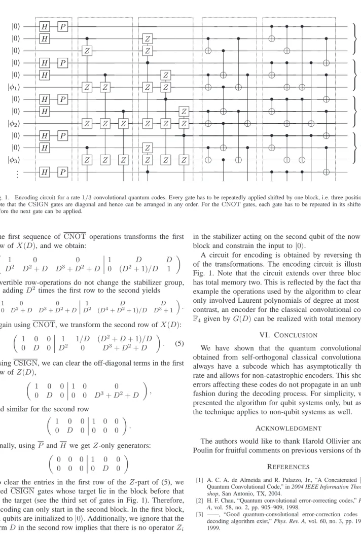
Fig. 1. Encoding circuit for a rate1/3convolutional quantum codes. Every gate has to be repeatedly applied shifted by one block, i.e. three positions down. Note that theCSIGNgates are diagonal and hence can be arranged in any order. For theCNOTgates, each gate has to be repeated in its shifted version before the next gate can be applied.
The first sequence of CNOT operations transforms the first row ofX(D), and we obtain:
1 0 0 1 D D
D2 D2+D D3+D2+D 0 (D2+ 1)/D 1
Invertible row-operations do not change the stabilizer group, so adding D2 times the first row to the second yields
1 0 0 1 D D
0 D2+D D3+D2+D D2 (D4+D2+ 1)/D D3+ 1
. Again usingCNOT, we transform the second row ofX(D):
1 0 0 1 1/D (D2+D+ 1)/D 0 D 0 D2 0 D3+D2+D
. (5)
UsingCSIGN, we can clear the off-diagonal terms in the first row ofZ(D), 1 0 0 1 0 0 0 D 0 0 0 D3+D2+D , and similar for the second row
1 0 0 1 0 0 0 D 0 0 0 0
. Finally, usingP andH we getZ-only generators:
0 0 0 1 0 0 0 0 0 0 D 0
To clear the entries in the first row of the Z-part of (5), we need CSIGN gates whose target lie in the block before that of the target (see the third set of gates in Fig. 1). Therefore, encoding can only start in the second block. In the first block, all qubits are initialized to|0i. Additionally, we ignore that the termD in the second row implies that there is no operatorZi
in the stabilizer acting on the second qubit of the now second block and constrain the input to |0i.
A circuit for encoding is obtained by reversing the order of the transformations. The encoding circuit is illustrated in Fig. 1. Note that the circuit extends over three blocks, i.e., has total memory two. This is reflected by the fact that in this example the operations used by the algorithm to clear entries only involved Laurent polynomials of degree at most two. In contrast, an encoder for the classical convolutional code over
F4 given byG(D)can be realized with total memory one. VI. CONCLUSION
We have shown that the quantum convolutional codes obtained from self-orthogonal classical convolutional codes always have a subcode which has asymptotically the same rate and allows for non-catastrophic encoders. This shows that errors affecting these codes do not propagate in an unbounded fashion during the decoding process. For simplicity, we have presented the algorithm for qubit systems only, but as in [8], the technique applies to non-qubit systems as well.
ACKNOWLEDGMENT
The authors would like to thank Harold Ollivier and David Poulin for fruitful comments on previous versions of the paper.
REFERENCES
[1] A. C. A. de Almeida and R. Palazzo, Jr., “A Concatenated[(4,1,3)]
Quantum Convolutional Code,” in 2004 IEEE Information Theory
Work-shop, San Antonio, TX, 2004.
[2] H. F. Chau, “Quantum convolutional error-correcting codes,” Phys. Rev.
A, vol. 58, no. 2, pp. 905–909, 1998.
[3] ——, “Good quantum-convolutional error-correction codes and their decoding algorithm exist,” Phys. Rev. A, vol. 60, no. 3, pp. 1966–1974, 1999.
[4] I. Daubechies and W. Sweldens, “Factoring Wavelet Transforms into Lifting Steps,” The journal of Fourier analysis and applications, vol. 4, no. 3, pp. 247–269, 1998.
[5] G. D. Forney, Jr. and S. Guha, “Simple Rate-1/3 Convolutional and Tail-Biting Quantum Error-Correcting Codes,” in Proceedings of the International Symposium on Information Theory (ISIT 05), 2005, pp. 1028–1032.
[6] G. D. Forney Jr., M. Grassl, and S. Guha, “Convolutional and tail-biting quantum error-correcting codes,” 2005, preprint quant-ph/0511016, sub-mitted to IEEE Transactions on Information Theory.
[7] M. Grassl and M. R¨otteler, “Quantum block and convolutional codes from self-orthogonal product codes,” in Proceedings of the International Symposium on Information Theory (ISIT 05), 2005, pp. 1018–1022.
[8] M. Grassl, Th. Beth, and M. R¨otteler, “Efficient quantum circuits for non-qubit quantum error-correcting codes,” International Journal of Foundations of Computer Science, vol. 14, no. 5, pp. 757–775, 2003. [9] R. Johannesson and K. S. Zigangirov, Fundamentals of Convolutional
Coding, ser. IEEE Series on Digital and Mobile Communication. New York: IEEE Press, 1999.
[10] M. Nielsen and I. Chuang, Quantum Computation and Quantum Infor-mation. Cambridge University Press, 2000.
[11] H. Ollivier and J.-P. Tillich, “Description of a quantum convolutional code,” Phys. Rev. Lett., vol. 91, no. 17, p. 177902, 2003.
[12] ——, “Quantum convolutional codes: fundamentals,” 2004, preprint quant-ph/0401134.