Meteorology Senior Theses Undergraduate Theses and Capstone Projects
12-2016
Multi-Radar Multi-Sensor Vs Single Radar Severe
Weather Observations
Garrett W. Starr
Iowa State University, [email protected]
Follow this and additional works at:https://lib.dr.iastate.edu/mteor_stheses
Part of theMeteorology Commons
This Dissertation/Thesis is brought to you for free and open access by the Undergraduate Theses and Capstone Projects at Iowa State University Digital Repository. It has been accepted for inclusion in Meteorology Senior Theses by an authorized administrator of Iowa State University Digital Repository. For more information, please [email protected].
Recommended Citation
Starr, Garrett W., "Multi-Radar Multi-Sensor Vs Single Radar Severe Weather Observations" (2016).Meteorology Senior Theses. 3.
1
Multi-Radar Multi-Sensor Vs Single Radar Severe Weather Observations Garrett W. Starr
Department of Geological and Atmospheric Sciences, Iowa State University, Ames, Iowa
Mentor – Dr. James V. Aanstoos
Iowa State University
ABSTRACT
Multi-Radar Multi-Sensor (MRMS) is a fairly new technology when considering how long storm systems have been analyzed by using radio detection and ranging (radar) processes. Unlike what most meteorologists use today, a MRMS system uses data from many surrounding radars along with information from sources such as rain gauges, surface observations, upper level observations, and more. This new system provides many new products for meteorologists to utilize when analyzing severe weather events, for example, tornadic storm cells. Often times when new technology like MRMS is presented, it provides many products not available on any other system; but exactly how useful are these new products when it comes to providing an actual advantage in real time severe weather analysis? This study was created to test the hypothesis that MRMS observations will provide a time advantage for issuing a tornado warning for a storm when comparing it to a single radar observation system. The two main products from each system up for comparison and analysis are the 0-2 kilometer above ground level(AGL) azimuth shear product from the MRMS system, and the storm relative velocity product from level II radar data. The study analyzes eight cases of tornado warned storm cells stretching from Iowa, down to Louisiana from the year 2016. After analyzing data from these eight cases, it can be concluded that MRMS technology does indeed provide a time advantage for meteorologists issuing tornado warnings.
______________________________________________________________________________
1. Introduction
Radio detection and ranging, or what is now commonly referred to as RADAR (or radar), has had a very long road from its beginning to the present day in terms of its uses and capabilities. The creation of one of the most useful tools to today’s meteorologists was actually an inadvertent
discovery made by scientists during World War II. The allied forces were trying to find ways to use radio detection and ranging to detect incoming enemy aircraft. In early July of 1940 a radar with a 10 centimeter wavelength was deployed in Wembley, England where a scientist by the name of Dr. J. W. Ryde worked. It is likely that the first weather echo, or backscattered energy, was
2
seen by this radar in late 1940 (Whiton et al. 1998). Ryde and the other scientists working at this facility found that when thunder storms moved into the area that they were scanning, that back scattered energy that was picked up by the radar antenna. This back scattered energy from these clouds and rain interfered with their ability to see possible aircraft over the same area, so the scientists were then tasked with investigating the attenuation and back scattering properties of clouds and rain (Whiton et al. 1998).
After the war, and as technology advanced new radar technology became available; the first radar that was designed and developed specifically for meteorologist and weather observations was deployed in the 1950’s. These radars are far less advanced that the radars that meteorologists know and use today. With these radars, after the backscattered energy was received by the radar, very little to no signal processing was used in order to calculate and output any other products. The WSR-57 (weather surveillance radar- 1957) was the world’s first ‘modern’ weather radar however it still only could provide course reflectivity data. One of the major down falls associated with WSR-57 was that it could not give the meteorologist using it any indication of how the winds associated with the storms were acting, which made it exceptionally difficult to identify possible tornados. As more time passed, the need for tornado detection capabilities continued to grow. New
technology and even more radar
electromagnetic signal processing procedures were created that gave meteorologist more advantages with real-time severe weather analysis. One of the most important steps
forward in radar was the development of Doppler radar. ‘Doppler’ radars were able to identify tornadic storms by showing meteorologist the radial components of the wind velocity with respect to the radar’s location. The Joint Doppler Operational Project (JDOP) determined that the use of these Doppler radars, “increases warning lead time for tornadoes from about 2 minutes to 20 minutes” (Whiton et al. 1998). Another major advancement in this field is the implementation of using both vertically and
horizontally polarized electromagnetic
waves, or Dual-Polarization (Dual-Pol) technology. Radars with dual-pol capability can show meteorologists real-time data about the sizes and shapes of the hydrometeors within a storm.
The most modern operational weather radar used today is the WSR-88D (weather surveillance radar 1988 doppler). This new radar was implemented throughout the 1990’s and is still being used today. This radar’s systems generate three basic meteorological quantities, which are the reflectivity, mean radial velocity, and spectrum width. Using these three base data quantities, the processing unit for the WSR-88D can calculate numerous meteorological analysis products that were not previously available with past radar systems (Klazura and Imy 1993). The combination of this radar new signal processing, dual-pol technologies, and Doppler radar capabilities made it second to none to any other radar system. This is also the radar that is most widely used by meteorologists around the United States. One of these new products is the ability measure the mean radial velocity, or the radial component of the wind either towards or
3
away from the radar. This product is mainly used for finding areas of tight rotation near the ground, usually indicative of a tornado. Another useful product available due to the radars dual-pol capabilities is the differential reflectivity or ZDR. This product help identifies the shape of the target. For example, more spherically shaped hail would have values near zero, while horizontally elongated rain drops would have a higher value of ZDR.
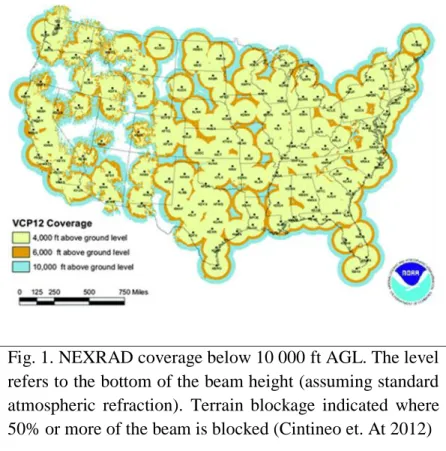
The coverage of these next generation radars (NEXRAD) is almost seamless across the entire United States (Fig. 1). Even though these radars are the most widely used and the most up to date, there has still been new developments in the field of radar meteorology; even in just the past few years. In recent years, rapid improvements in computer technology has made it possible to transfer high-volume data from multiple sources to a central location for the combination and processing of said data. This lead to the development of a new system called Multi-Radar Multi-Sensor (MRMS). MRMS provides many advantages when compared to looking at data from a single WSR-88D radar, in terms of real-time severe weather analysis and Quantitative Precipitation Estimation (QPE). MRMS integrates about 180 weather radars from the conterminous U.S. and Canada into a seamless nationwide 3 dimensional radar mosaic with a very high spatial and temporal resolution, being 1km and 2 minutes respectively (Zhang et al. 2016). The MRMS system was deployed to the National Center for Environmental Prediction in 2014 (Smith et al. 2016). It
provided many new products that could enhance how meteorologist analyze severe weather events. One of these brand-new products, as described in (Smith et al 2016) is called azimuthal shear. The azimuthal shear product finds the rotational component of the radial velocity at two different levels, 0-2km and 3-6 km above ground level. Analyzing the azimuthal shear product can be useful for locating rotation within the atmosphere close to the ground, such as a tornado, as well as detecting a rotating mesocyclone such as a larger scale supercell thunderstorm (MRMS Products Guide). Current studies have shown that all these new products can be very useful to severe weather analysis. However, all sources aforementioned have not looked at how these new products given to them through MRMS technology could increase the lead times for tornado warnings, or in how using
Fig. 1. NEXRAD coverage below 10 000 ft AGL. The level refers to the bottom of the beam height (assuming standard atmospheric refraction). Terrain blockage indicated where 50% or more of the beam is blocked (Cintineo et. At 2012)
4
these products could provide a time
advantage when trying to predict other key meteorological features. This study will attempt to bridge this gap in current knowledge by looking at how these new MRMS products can affect lead times for tornado warnings, specifically focusing on the azimuth shear 0-2km AGL product and how it impacts the severe weather analysis.
2. Data and Analytical Methods
a) Data Acquisition and Viewing
The first order of business that needed to be taken care of for this study to take place was to find the necessary data in order to properly analyze several different case studies to see if there was indeed a time advantage for issuing tornado warnings when using MRMS data to analyze severe weather events. To compare MRMS to single radar observations, data from both technologies was needed. The single radar level II data was acquired using the National Oceanic and Atmospheric Administration’s (NOAA)
National Centers for Environmental
Information (NCEI) archive information request system to order the radar data online for a specific radar site. Once the data was received by email, it was downloaded using FileZilla and then the .TAR files were unzipped. Once unzipped they were ready to be viewed in a level II data viewing system. The level II radar data viewing system that was used for this study was Gibson Ridge level 2 Analyst from Gibson Ridge Software, LLC. This GR2Analyst system allowed the level II radar data to be viewed nicely for analysis.
To view the Multi-Radar Multi-Sensor data, the site that was the most effective to use was the mrms.ou.edu site. The data did not have to be ordered for a specific radar location because MRMS technology offers a seamless radar coverage pattern in most areas. Also no data had to be ordered at all with this site, it was all available in real time for the viewers. Once on the site, the single product map viewer was used to observe the next generation (NextGen) products. In the list of provided NextGen products was the main product needed for this study, the 0-2km AGL azimuth shear parameter. More NextGen products that were used in this study were the Composite Reflectivity (CREF), and the Base Reflectivity (BREF) products. This site allowed the MRMS data to be viewed on loop, or to be stopped on each individual scan which was updated every 2 minutes. One problem that this site possessed was that it limited the case study choices significantly. One of the main advantages of using MRMS data for severe weather analysis is that it provides new scans to be viewed every 2 minutes as opposed to new scans roughly 5 minutes with single radar observations. Since MRMS is a relatively new technology, some difficulties were ran into with this site. Only data that was after late August, early September 2016 was available with the 2-miunte temporal resolution. That being said, the cases available to choose from would have to be after those dates.
A total of eight separate cases were chosen for this study. Since the main focus of this study was to see how this new MRMS technology could affect the times that tornado warnings were issued, each case
5
chosen must have had been under a tornado warning at some time. These studies occurred in various locations, days, and were different storm type setups, such as a quasi-linear convective system or super cell thunderstorm (Table 1). Note that some storm cell cases were observed by the same radar sites on the same days. Some hours to just mere minutes apart. Due to the fact that the naming convention for these cases was the name of the site of the radar that they were observed by, radar sites that observed multiple tornado warned storms that were analyzed by this study are named as such; XXXXa and XXXXb.
b) Methods of Analysis
To analyze these case studies, three main pieces of information were needed to fulfill the goal of this study. The first piece of information that was needed to be found was when the earliest time that there was a radar radial velocity couplet visible on the level II radar images. A radar radial velocity couplet is an area located in the storm where there is a very tight region of pixels on the radar’s display of winds moving towards and away from the radar, indicating an area of tight small scale circulation. To find this, the level II radar data was loaded in GR2Analyst, and then the storm cells were located. Once the proper cells were located the level II product Table 1. Shown below are the details for each of the eight cases analyzed in this study
Radar Site Location Date Case Name for This
Study
KDVN NW of Muscatine, Iowa 10-6-2016 Case KDVNa
KDVN Davenport, Iowa 10-6-2016 Case KDVNb
KDMX North Central Iowa 9-21-2016 Case KDMX
KICT South Central Kansas 10-6-2016 Case KICT
KINX SE Kansas, NE Oklahoma 10-6-2016 Case KINX
KPOE Central Louisiana 11-28-2016 Case KPOEa
KPOE Central Louisiana 11-28-2016 Case KPOEb
6
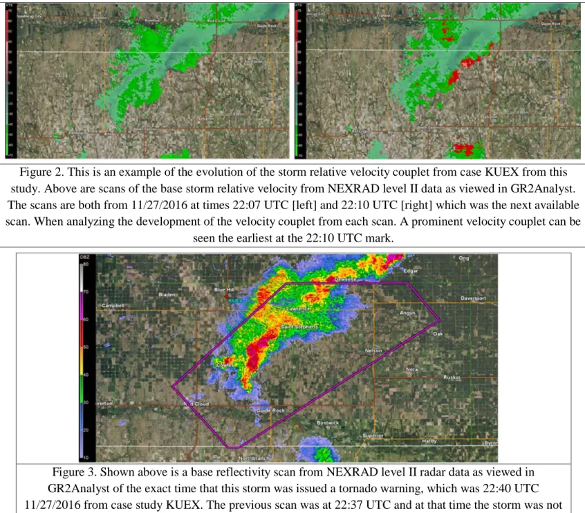
that was used to find this velocity couplet was the storm relative velocity or SRV. SRV is a product that takes the base velocity (BV) of the storm, or the storms radial motion toward or away from the radar, and takes away from those BV values from the magnitude of the average storm motion. Thus giving a more accurate representation of the true wind velocities within the storm (Fig. 2).
The second main piece of information required to complete the analysis was at what point in time for each case was the tornado warning issued. To find this piece of information, the level II data was loaded into GR2Analyst. Once loaded in to the level II data viewer, the radar loop could be played through up to the point where the viewer could see when the
Figure 2. This is an example of the evolution of the storm relative velocity couplet from case KUEX from this study. Above are scans of the base storm relative velocity from NEXRAD level II data as viewed in GR2Analyst. The scans are both from 11/27/2016 at times 22:07 UTC [left] and 22:10 UTC [right] which was the next available scan. When analyzing the development of the velocity couplet from each scan. A prominent velocity couplet can be
seen the earliest at the 22:10 UTC mark.
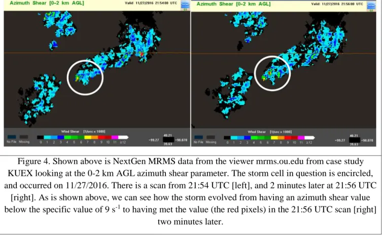
Figure 3. Shown above is a base reflectivity scan from NEXRAD level II radar data as viewed in GR2Analyst of the exact time that this storm was issued a tornado warning, which was 22:40 UTC 11/27/2016 from case study KUEX. The previous scan was at 22:37 UTC and at that time the storm was not
7
exact time and location that the tornado warning was issued (Fig. 3).
The final and most important piece of information for the comparison of single radar observations to MRMS observations was in regards to the 0-2 km AGL azimuth shear parameter. To use this parameter to compare these observations, a certain value of this azimuth shear parameter needed to be chosen such that the value was indicative of potential tornadic activity. The value for this study was decided on was 9 s-1. This was chosen because in a figure in the Weather Decision Training Division’s 2016 MRMS Products Guide, a confirmed tornadic supercell over Kansas on April 14 2012 showed values of 9 s-1. Certainly tornadic supercells can reach higher values than 9 s-1, as did many of the cases in this study. However, sometimes these higher values
occurred when a very prominent velocity couplet was also able to be viewed simultaneously. If this study used a value such as 12 s-1 there would likely be less of a time advantage when issuing tornado warnings with that data when we know that tornadic activity can occur with values as low as 9 s-1, so using a value of 12 s-1 would be an unnecessarily high option. So now that a criteria was chosen for the azimuth shear parameter, the time in which the
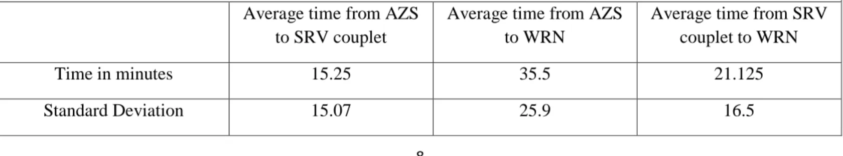
corresponding storm’s azimuth shear levels reached the aforementioned level of 9 s-1 was needed to be found. Using the MRMS data viewer as mentioned above, the data was stepped through scan by scan until the exact time that the 0-2 km AGL azimuth shear reached the level of 9 s-1 (Fig. 4).
Figure 4. Shown above is NextGen MRMS data from the viewer mrms.ou.edu from case study KUEX looking at the 0-2 km AGL azimuth shear parameter. The storm cell in question is encircled, and occurred on 11/27/2016. There is a scan from 21:54 UTC [left], and 2 minutes later at 21:56 UTC
[right]. As is shown above, we can see how the storm evolved from having an azimuth shear value below the specific value of 9 s-1 to having met the value (the red pixels) in the 21:56 UTC scan [right]
8
3. Results and Discussion a) Results
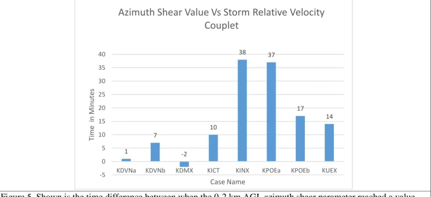
Once all three data points for each of the eight cases were found, the times that each of the respective circumstances took place could be compared and analyzed. Those circumstances again being, the time of the first visible prominent storm relative velocity couplet, when the tornado warnings were issued, and when the azimuth shear parameter reached its chosen critical value of 9 s-1 for every case. The results for this study are most easily comprehended when looked at in graphical form. The main comparisons made in this study were as follows; What was the time difference between when the 0-2 km AGL azimuth shear parameter reached a value on 9 s-1 and when the first visible storm relative velocity couplet appeared (Fig.5), and what was the time difference between when the 0-2 km AGL azimuth shear parameter reached a value on 9 s-1 and when the tornado warning was issued (Fig. 6).
After doing further analysis of the time differences, the average time advantages and standard deviations were calculated (Table 2).
a) Discussion
When looking at the time difference between when the 0-2 km AGL azimuth shear parameter reached a value on 9 s-1 and when the first SRV couplet was visible (Fig. 5), in all but one case the azimuth shear indicated the storm was exhibiting tornadic behaviors before a SRV couplet was even visible. Also when comparing those two values, the average time advantage of seeing when a storm cell was possibly a tornadic storm cell was 15.25 minutes. When
comparing the time that the azimuth shear reached the necessary value to when an actual tornado warning was issued, the average time difference was 35.5 minutes. A strong SRV couplet is a very good indicator if there is a tornado present within the storm. The azimuth shear parameter is also a good indicator if there is a possibility of a tornado being present within a storm. With that being said, using MRMS data such as the azimuth shear parameter could provide more of a lead time for issuing a tornado warning. When looking at each
individual case study, it can be seen that a trend in the data is present. The time difference between when the azimuth
Table 2. AZS in this table refers to the when the 0-2 km AGL azimuth shear parameter reached a value on 9 s-1. SRV couplet refers to when the first SRV couplet was visible on the radar display. WRN refers to the time that the tornado warning was issued for each storm. The calculations done were the average time differences between the two data points listed in the box’s description. Also calculated were the standard deviations of each data set.
Average time from AZS
to SRV couplet
Average time from AZS to WRN
Average time from SRV couplet to WRN
Time in minutes 15.25 35.5 21.125
9
Figure 5. Shown is the time difference between when the 0-2 km AGL azimuth shear parameter reached a value on 9 s-1 and when the first visible SRV couplet appeared. Time 0 represents the time when the azimuth shear reached its given value of 9 s-1. The bars represent the number of minutes before or after that time when the first SRV couplet was visible.
Figure 6. Shown is the time difference between when the 0-2 km AGL azimuth shear parameter reached a value on 9 s-1 and when the tornado warning was issued. Time 0 represents the time when the azimuth shear reached its given value of 9 s-1. The bars represent the number of minutes after that time when the tornado warning was issued. 1 7 -2 10 38 37 17 14 -5 0 5 10 15 20 25 30 35 40
KDVNa KDVNb KDMX KICT KINX KPOEa KPOEb KUEX
Ti me in M in u tes Case Name
Azimuth Shear Value Vs Storm Relative Velocity
Couplet
10
shear critical value was reached and when both the SRV couplet was visible and when the tornado warning is noticeably greater for cases KINX, KPOEa, KPOEb, and KUEX. This may be due to the fact that these radar sites were in areas where the radar site density was greater than that for the other cases selected that produced less of a time difference. Since MRMS
observations pull data from multiple different radar locations along with other sources, the conclusion can be drawn that areas with more sources of data input for the MRMS system, the more accurate the MRMS products will be. As shown by this study, areas with a more accurate MRMS system provided even greater time differences between when the azimuth shear parameter reached 9 s
-1 and when both the SRV couplet was
present and the tornado warning was issued. This only further supports the fact that the MRMS system could benefit forecasters in issuing tornado warnings for the public.
4. Conclusion
Looking at all the cases analyzed in this study as a whole, it can be said that using an MRMS system would provide a possible time advantage to forecasters in regards to issuing a tornado warning. When comparing the individual abilities of the single level II radar data products to the MRMS system’s products with these case studies, a clear advantage can be seen. When using the SRV to see if a tornado could be present in a storm, the time difference between seeing
the SRV couplet and the issuing of the tornado warning was 21.125 minutes. On the other hand, if the azimuth shear product was used to indicate if a storm was possibly tornadic, the time difference between seeing the critical value of 9 s-1 and the issuing of
the tornado warning was 35.5 minutes. When looking the comparison between these two time differences, it can be seen that using the MRMS azimuth shear product over the SRV couplet to determine if the storm is possibly tornadic yields an average possible time advantage for issuing a tornado warning on a storm of 14.375 minutes. A 14.375 minute advantage is significant when considering that every minute counts when the public is seeking shelter from an incoming storm. In this world, with technology rapidly evolving the way that it is, it is possible that the MRMS system could one day replace the single radar observations that most severe weather analysts use today.
5. Acknowledgements
I would like thank Dr. James V. Aanstoos for his guidance on this study. I would also like to thank David Flory for his assistance in obtaining and viewing the level II radar data that made this study possible
References
Cintineo, J., T. Smith, V. Lakshmanan, H. Brooks, and K. Ortega, 2012: An Objective High-Resolution Hail
11
Climatology of the Contiguous United States.Wea.
Forecasting,27, 1235–1248, doi: 10.1175/WAF-D-11-00151.1. Klazura, G. and D. Imy, 1993: A
Description of the Initial Set of Analysis Products Available from the NEXRAD WSR-88D System. Bull. Amer. Meteor. Soc., 74, 1293– 1311, doi:
10.1175/1520-0477(1993)074<1293:ADOTIS>2.0. CO;2.
Smith, T., V. Lakshmanan, G. Stumpf, K. Ortega, K. Hondl, K. Cooper, K. Calhoun, D. Kingfield, K. Manross, R. Toomey, and J. Brogden, 2016: Multi-Radar Multi-Sensor (MRMS) Severe Weather and Aviation Products: Initial Operating Capabilities. Bull. Amer. Meteor. Soc., 97, 1617–1630, doi:
10.1175/BAMS-D-14-00173.1. The Weather Decision Training Division,
2016: MRMS Products Guide. 9/09/2016,
http://www.wdtb.noaa.gov/courses/ MRMS/ProductGuide/index.php/BA MS-D-14-00174.1
Whiton, R., P. Smith, S. Bigler, K. Wilk, and A. Harbuck, 1998: History of Operational Use of Weather Radar by U.S. Weather Services. Part I: The Pre-NEXRAD Era. Wea. Forecasting, 13, 219–243, doi:
10.1175/1520-0434(1998)013<0219:HOOUOW>2. 0.CO;2.
Whiton, R., P. Smith, S. Bigler, K. Wilk, and A. Harbuck, 1998: History of Operational Use of Weather Radar by U.S. Weather Services. Part II: Development of Operational Doppler Weather Radars. Wea. Forecasting, 13, 244–252, doi: 10.1175/1520-0434(1998)013<0244:HOOUOW>2. 0.CO;2
Zhang, J., K. Howard, C. Langston, B. Kaney, Y. Qi, L. Tang, H. Grams, Y. Wang, S. Cocks, S. Martinaitis, A. Arthur, K. Cooper, J. Brogden, and D. Kitzmiller, 2016: Multi-Radar Multi-Sensor (MRMS) Quantitative Precipitation Estimation: Initial Operating Capabilities. Bull. Amer. Meteor. Soc., 97, 621–638, doi: 10.1175/BAMS-D-14-00174.1.