Methodological Issues in Spatial Microsimulation Modelling for Small Area Estimation

Methodological Issues in Spatial Microsimulation Modelling for

Small Area Estimation

Azizur Rahman*, Ann Harding, Robert Tanton and Shuangzhe Liu

National Centre for Social and Economic Modelling (NATSEM), University of Canberra, ACT 2601, Australia; *email: [email protected]

ABSTRACT: In this paper, some vital methodological issues of spatial microsimulation modelling for small area estimation have been addressed, with a particular emphasis given to the reweighting techniques. Most of the review articles in small area estimation have highlighted methodologies based on various statistical models and theories. However, spatial microsimulation modelling is emerging as a very useful alternative means of small area estimation. Our findings demonstrate that spatial microsimulation models are robust and have advantages over other type of models used for small area estimation. The technique uses different methodologies typically based on geographic models and various economic theories. In contrast to statistical model-based approaches, the spatial microsimulation model-based approaches can operate through reweighting techniques such as GREGWT and combinatorial optimization. A comparison between reweighting techniques reveals that they are using quite different iterative algorithms and that their properties also vary. The study also points out a new method for spatial microsimulation modelling

Keywords: Bayesian prediction approach; combinatorial optimisation; GREGWT; microdata; small area estimation; spatial microsimulation

1. INTRODUCTION

Small area estimation is the method of estimating reliable statistics at the small geographical area or a spatial micropopulation unit. Reliable statistics of interest at small area levels cannot be ordinarily and directly produced, due to certain limitations of the available data. For instance, a suitable sample that contains enough representative observations is typically not available for all small areas from national level survey data. A basic problem with national or state level surveys is that they are not designed for efficient estimation for small areas (Heady et al., 2003). In practice, small area estimates from these national sample surveys are statistically unreliable, due to sample observations being insufficient, or in many cases non-existent, where the domain of interest may fall outside the sample domains (Tanton, 2007). Given typical time and money constraints, it is usually impossible to conduct a sufficiently comprehensive survey to get enough data from every small area we are interested in.

Nowadays indirect modelling approaches of small area estimation, such as spatial microsimulation models (SMMs), have received much attention, due to their usefulness and the increasing demand for reliable small area statistics from both private and public level organisations. In these approaches, one uses data from similar domains to estimate the statistics in a particular small area of interest, and this „borrowing of strength‟ is justified by assuming a model that relates the small area statistics (Meeden, 2003). Typically, indirect small area estimation is the process of using statistical models and/or geographic models to link survey outcome or response variables to a set of predictor variables known for small areas, in order to predict small area estimates. As a result of inadequate sample observations in small geographic areas, the conventional area-specific direct estimates may not provide enough

statistical precision. In such a situation, an indirect model-based method can produce better results.

Most of the review articles in small area estimation have highlighted the methodologies, which are fully based on various statistical models and theories (for example, Ghosh and Rao, 1994; Rao, 1999; Pfeffermann, 2002; Rao, 2002; Rao, 2003a). However another type of technique called „spatial microsimulation modelling‟ has been used in providing small area estimates during the last decade (for instance, Williamson et al., 1998; Ballas et al., 2003; Taylor et al., 2004; Brown and Harding, 2005; Chin et al., 2005; Ballas et al., 2006; Chin and Harding, 2006; Cullinan et al., 2006; Lymer et al., 2006; Anderson, 2007; Chin and Harding, 2007; King, 2007; Tanton, 2007) . The SMMs are based on geographic and economic theories, and their methodologies are quite different from other statistical approaches. Although these approaches are frequently used in social and economic analysis, and seem to be a robust and rational indirect modelling tool, the mechanisms behind them are not always well documented. Also there are some important methodological issues where more research should improve the performance of SMMs and help in the validation of their estimates.

This paper provides a brief synopsis of the overall methodologies for small area estimation and explicitly addresses some vital methodological issues of spatial microsimulation modelling, with a particular emphasis given to the reweighting techniques. It also proposes a new approach in the SMM methodologies. An application of the generalised regression based reweighting technique discussed in this article is studied by Tanton and Vidyattama under distinct features of the applicable data. This contribution is part of this special issue as well.

RAHMAN, HARDING, TANTON AND LIU Methodological issues in spatial microsimulation modelling 4 There are 5 sections within this paper. In Section

2, a diagramic representation of the overall methodologies in small area estimation is provided with a synopsis of various direct and indirect statistical model based estimations, and highlights of spatial microsimulation modelling. In Section 3, some vital methodological issues in spatial microsimulation modelling are addressed, which include theories and numerical solutions of different reweighting techniques. In Section 4, a comparison between two reweighting techniques is presented with a new methodology for generating small area microdata. Finally, conclusions are given in Section 5.

2. METHODS OF SMALL AREA ESTIMATION: AN OVERALL VIEW

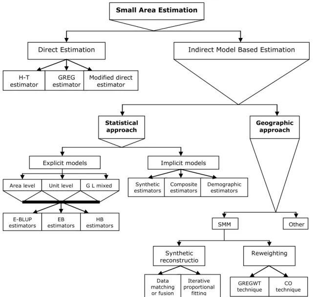
A diagramic representation of the overall methodologies for small area estimation is depicted in Figure 1. Traditionally there are two types of small area estimation – direct and indirect estimation. Direct small area estimation is based on survey design and includes three estimators

called the Horvitz-Thompson estimator, GREG estimator and modified direct estimator. On the other hand, indirect approaches of small area estimation can be divided into two classes – statistical and geographic approaches. The statistical approach is mainly based on different statistical models and techniques. However, the geographic approach uses techniques such as SMMs.

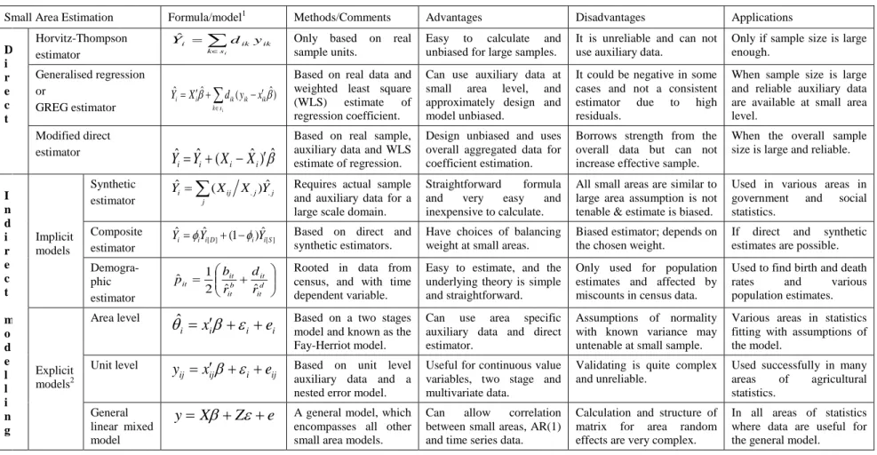
It is noted that implicit model based statistical approaches include three types of estimators, which are synthetic, composite and demographic estimators. Whereas, there are also three kinds of explicit models categorized as area level, unit level and general linear mixed models. Based on the type of study researchers are interested in, each of these models is widely applied to obtained small area indirect estimates by utilising the (empirical-) best linear unbiased prediction (E-BLUP), empirical Bayes (EB) and hierarchical Bayes (HB) methods. A very brief synopsis of different direct and indirect statistical model based small area estimation techniques is presented in Table 1 (for details, see Rahman, 2008a).

Figure 1 A summary of different techniques for small area estimation

(after Rahman, 2008a). Explicit models

Indirect Model Based Estimation Direct Estimation

H-T

estimator estimator GREG Modified direct estimator

Small Area Estimation

Statistical approach

Implicit models

Synthetic

estimators Composite estimators Demographic estimators

E-BLUP

estimators estimators EB estimators HB Area level Unit level G L mixed

Geographic approach SMM Other Synthetic reconstructio n Reweighting CO technique GREGWT technique Iterative proportional fitting Data matching or fusion

Table 1 A brief summary of different methods for direct and indirect statistical model based small area estimation.

Small Area Estimation Formula/model1 Methods/Comments Advantages Disadvantages Applications

D i r e c t Horvitz-Thompson estimator



  i s k ik ik i d y

Yˆ Only based on real sample units.

Easy to calculate and unbiased for large samples.

It is unreliable and can not use auxiliary data.

Only if sample size is large enough. Generalised regression or GREG estimator



      i s k ik ik ik i i X d y x Yˆ ˆ ( ˆ)

Based on real data and weighted least square (WLS) estimate of regression coefficient.

Can use auxiliary data at small area level, and approximately design and model unbiased.

It could be negative in some cases and not a consistent estimator due to high residuals.

When sample size is large and reliable auxiliary data are available at small area level. Modified direct estimator

_

ˆ

)

ˆ

(

ˆ

ˆ

_

_

_

_

i i i i

Y

X

X

Y

Based on real sample, auxiliary data and WLS estimate of regression.

Design unbiased and uses overall aggregated data for coefficient estimation.

Borrows strength from the overall data but can not increase effective sample.

When the overall sample size is large and reliable.

I n d i r e c t m o d e l l i n g Implicit models Synthetic estimator



 j j j ij i X X Y

Yˆ ( _. )ˆ_. Requires actual sample

and auxiliary data for a large scale domain.

Straightforward formula and very easy and inexpensive to calculate.

All small areas are similar to large area assumption is not tenable & estimate is biased.

Used in various areas in government and social statistics. Composite estimator [ ] [] ˆ ) 1 ( ˆ ˆ S i i D i i i Y Y

Y    Based on direct and

synthetic estimators.

Have choices of balancing weight at small areas.

Biased estimator; depends on the chosen weight.

If direct and synthetic estimates are possible. Demogra-phic estimator         _d it it b it it it r d r b p ˆ ˆ 2 1

ˆ Rooted in data from _{census, and with time} dependent variable.

Easy to estimate, and the underlying theory is simple and straightforward.

Only used for population estimates and affected by miscounts in census data.

Used to find birth and death rates and various population estimates. Explicit models2 Area level i i i i



x











e



ˆ

Based on a two stages model and known as the Fay-Herriot model.

Can use area specific auxiliary data and direct estimator.

Assumptions of normality with known variance may untenable at small sample.

Various areas in statistics fitting with assumptions of the model. Unit level ij i ij ij

x

e

y













Based on unit level auxiliary data and a nested error model.

Useful for continuous value variables, two stage and multivariate data.

Validating is quite complex and unreliable.

Used successfully in many areas of agricultural statistics. General linear mixed model

e

Z

X

y











A general model, which encompasses all other small area models.

Can allow correlation between small areas, AR(1) and time series data.

Calculation and structure of matrix for area random effects are very complex.

In all areas of statistics where data are useful for the general model.

1

All usual notations are utilized (see Rahman, 2008a for details).

2

Methods such as empirical best linear unbiased predictor (E-BLUP), empirical Bayes (EB) and hierarchical Bayes (HB) are frequently used in explicit model based small area estimation. An excellent discussion of each of these complex methods is given in Rao (2003), and also in Rahman (2008a).

RAHMAN,HARDING,TANTON AND LIU Methodological issues in spatial microsimulation modelling 6 However, in contrast to statistical approaches, the

geographic approach is based on microsimulation models, which are essentially creating synthetic/simulated micro-population data to produce „simulated estimates‟ at small area level. To obtain reliable microdata at small area level is the key task for spatial microsimulation modelling. Synthetic reconstruction and reweighting are two commonly used methods in microsimulation, and each of them is stimulated by different techniques to produce simulated estimators. As the main objective of this paper is to discuss the methodological issues of spatial microsimulation modelling, the subsequent sections will encompass those methods for explicit treatments.

2.1 SMM estimation

The Spatial Microsimulation Model (SMM) approach to small area estimation harks back to the microsimulation modelling ideas pioneered in the middle of last century by Guy Orcutt (1957, 2007). This approach is fully based on SMMs and also known as the geographic method. During the last two decadesmicrosimulation modelling has become a popular, cost-effective and accessible method for socioeconomic policy analysis, with the rapid development of increasingly powerful computer hardware; the wider availability of individual unit record datasets (Harding, 1993, 1996); and with the growing demand (Harding and Gupta, 2007) for small area estimates at government and private sectors.

Microsimulation modelling was originally developed as a tool for economic policy analysis (Merz, 1991). Clarke and Holm (1987) provide a thorough presentation on how microsimulation methods can be applied in regional science and planning analysis. According to Taylor et al. (2004), spatial microsimulation can be conducted by re-weighting a generally national level sample so as to estimate the detailed socio-economic characteristics of populations and households at a small area level. This modelling approach combines individual or household microdata, currently available only for large spatial areas, with spatially disaggregate data to create synthetic microdata estimates for small areas (Harding et al., 2003). Various microsimulation models such as static, dynamic and spatial

microsimulation models are discussed in the literature (Harding, 1996; Harding and Gupta, 2007).

Although microsimulation techniques have become useful tools in the evaluation of socioeconomic policies, they involve some complex subsequent procedures. An overall process involved with spatial microsimulation is described in detail by Chin and Harding (2006). They classified two major steps within this process, which are first, to create household weights for small areas using a reweighing method and, second, to apply these household weights to the selected output variables to generate small area estimates of the selected variables. Further, each of these major steps involve several sub-steps (Chin and Harding 2006). Ballas et al. (2005) outline four major

steps involved with a microsimulation process, which are:

 the construction of a „microdata‟ set (when this is not available);

 Monte Carlo sampling from this data set to „create‟ a micro level population (or a „synthetic‟ population (see, Chin and Harding, 2006)) for the interested domain;

 what-if simulations, in which the impacts of alternative policy scenarios on the population are estimated; and

 dynamic modelling to update a basic microdata set.

The starting point for microsimulation models is a microdata file, which provides comprehensive information on different characteristics of individual persons, families or households in the file. In Australia, microdata are generally available in the form of confidentialised unit record files (CURFs) from the Australian Bureau of Statistics (ABS) national level surveys. Typically, the survey data provide a very large number of variables and an adequate sample size to allow statistically reliable estimates for only large domains (such as only at the broad level of the state or territory). Small area estimates from these national sample surveys are statistically unreliable because of sample observations being insufficient or in many cases non-existent where the domain of interest may fall out of the sample areas. For example if a land development agency wants to develop a new housing domain/suburb, then this new small domain should be out of the sample areas. Also, in order to protect the privacy of the survey respondents, national microdata often lack a geographical indicator which, if present, is often only at the wide level of the state or territory (Chin and Harding, 2006). Therefore spatial microdata are usually unavailable and they need to be synthesized (Chin et al., 2005). The lack of spatially explicit microdata has in the past constrained of SMM for modelling of social policies and human behaviour.

One advantage of SMMs relative to the more traditional statistical small area estimation approaches is that the microsimulation models can be used for estimating the local or small area effects of policy change and future small area estimates of population characteristics and service needs (Williamson et al., 1998; Ballas et al., 2003; Taylor et al., 2004; Brown and Harding, 2005; Chin et al., 2005; Ballas et al., 2006; Chin and Harding, 2006; Cullinan et al., 2006; Lymer et al., 2006; Anderson, 2007; Chin and Harding, 2007; King, 2007; Tanton, 2007). For instance, spatial microsimulation may be of value in estimating the distributions of different population characteristics such as income, tax and social security benefits, income deprivation, housing unaffordability, housing stress, housing demand, care needs, etc. at small area level, when contemporaneous census and/or survey data are unavailable (Taylor et al., 2004; Chin et al., 2005; Lymer et al., 2006; Anderson, 2007; Tanton, 2007; Lymer et al., 2008; Harding et al., 2009).

This type of model is mainly intended to explore the relationships among regions and sub-regions and to project the spatial implications of economic development and policy changes at a more disaggregated level. Moreover spatial microsimulation modelling has some advanced features, which can be highlighted as:

 spatial microsimulation models are flexible in terms of the choice of spatial scale;

 they can allow data from various sources to create a microdata base file at the small area level;

 the models store data efficiently as lists of objects;

 spatial microdata have the potential for further aggregation or disaggregation; and

 models allow for updating and projecting. Thus, from some points of view, spatial microsimulation exploits the benefits of object-oriented planning, both as a tool and a concept. Spatial microsimulation frameworks use a list-based approach to microdata representation where a household or an individual has a list of attributes that are stored as lists rather than as occupancy matrices (Williamson et al., 1996). From a computer programming perspective, the list-based approach uses the tools of object-oriented programming because the individuals and households can be seen as objects with their attributes as associated instance variables. Alternatively, rather than using an object orientated programming approach, a programming language like SAS can also be used to run spatial microsimulation. For a technical discussion of the SAS-based environment used in the development of the STINMOD model and adapted to run other NATSEM regional level models, readers may refer to the technical paper by Chin and Harding (2006). Furthermore, by linking spatial microsimulation with static microsimulation we may be able to measure small area effects of policy changes, such as changes in government programs providing cash assistance to families with children (Harding et al., 2009). Another advantage of SMMs is the ability to estimate the geographical distribution of socio-economic variables, which were previously unknown (Ballas, 2001).

However spatial microsimulation adds to the simulation a spatial dimension, by creating and using synthetic microdata for small areas, such as SLA levels in Australia (Chin et al., 2005). There is often great difficulty in obtaining household microdata for small areas, since spatially disaggregate reliable data are not readily available. Even if these types of data are available in some form, they typically suffer from severe limitations – in either lack of characteristics or lack of geographical detail. Therefore, spatial microdata should be simulated, and that can be achieved by different probabilistic as well as deterministic methods.

3. METHODOLOGICAL ISSUES IN SMM As mentioned calculating statistically reliable

population estimates in a local area using survey microdata is challenging, due to the lack of enough sample observations. To create a synthetic spatial microdata set is one of the possible solutions. Simulation based methods can deal with such a problem by (re)weighting each respondent in the survey data, to create the synthetic spatial microdata. However, it is not easy process to create reliable spatial microdata. Complex methodologies are associated with the process. This section presents some of the vital methodological issues in spatial microsimulation modelling.

3.1 Creation of synthetic spatial microdata Methods for creating synthetic spatial microdata are mainly classified into the synthetic reconstruction and reweighting methods. Synthetic reconstruction is an older method, which attempts to construct synthetic micro-populations at the small area level in such a way that all known constraints at the small area level are reproduced. There are two ways of undertaking synthetic reconstruction - data matching or fusion (Moriarity and Scheuren, 2003; ABS, 2004; Tranmer et al., 2005) and iterative proportional fitting (Birkin and Clarke, 1988; Duley, 1989; Williamson, 1992; Norman, 1999). In contrast, the reweighting method, which is a relatively new and popular method, mainly calibrates the sampling design weights to a set of new weights based on a distance measure, by using the available data at spatial scale.

Data matching or fusion is a multiple imputation technique often useful to create complementary datasets for microsimulation models. Data collected from two different sources may be matched using variables (such as name and address or different IDs), which uniquely identify an individual or household. This type of data matching is commonly known as „exact matching‟. But, due to data confidentiality constraints, these unique identifier variables may not be available in all cases (for example, sample units or households in microdata such as CURFs of the ABS used in NATSEM cannot be identified because of the existence of data privacy legislation when gathering data from the population). For such a case, records from different datasets can also be „matched‟ if they share a core set of common characteristics. In general, the data matching technique involves a few empirical steps:

 adjusting available data files and variable transformations;

 choosing the matching variables;

 selecting the matching method and associated distance function; and

 validating.

A description of these empirical steps and theories behind them are available elsewhere (Alegre et al., 2000; Rassler, 2002). Details about data matching techniques are given by Rodgers (1984). Moreover, this tool is used to create microdata files by researchers in many countries, such as Moriarity and Scheuren (2001, 2003) in the USA;

RAHMAN, HARDING, TANTON AND LIU Methodological issues in spatial microsimulation modelling 8

Table 2 Synthetic reconstruction versus the reweighting technique

Liu and Kovacevic (1997) in Canada; Alegre et al. (2000), Tranmer et al. (2005), Rassler (2004) in Europe; and ABS (2004) in Australia, among many others.

Besides, the iterative proportional fitting (IPF) tool initially proposed by Deming and Stephan (1940). The authors developed the method for adjusting cell frequencies in a contingency table based on sampled observations subject to known expected marginal totals. This method has been used for several decades to create synthetic microdata from a variety of aggregate data sources. The theoretical and practical considerations behind this method have been discussed in several studies (Fienberg, 1970; Evans and Kirby, 1974; Norman, 1999), and the usefulness of this approach in spatial analysis and modelling has been revealed by Birkin and Clarke (1988), Wong (1992), Ballas et al. (1999) and Simpson and Tranmer (2005). The study by Wong (1992) also considers the reliability issues of using the IPF procedure and demonstrates that the estimates of individual level data generated by this process using data of equal-interval categories other than equal-size categories are more reliable, and the performance of the estimation can be improved by increasing sample size.

Previous to the development of „reweighting‟ techniques, the iterative proportional fitting procedure was a very popular tool to generate small area microdata. A summary of literature using this technique has been provided by Norman (1999). It appears from the study that almost all of the researchers in the United Kingdom were devoted to using the iterative proportional fitting procedure in microsimulation modelling. But nowadays most of the researchers are claiming that reweighting procedures have some advantages over the synthetic reconstruction approach (Williamson et al., 1998; Huang and Williamson, 2001; Ballas et al., 2003). A summary of the key issues associated with the two approaches is shown in Table 2.

Moreover, reweighting is a procedure used throughout the world to transform information contained in a sample survey to estimates for the micro population (Chin and Harding, 2006). For example, the Australian Bureau of Statistics calculates a weight (or „expansion factor‟) for each of the 6,892 households included in the 1998-99 Household Expenditure Survey sample file (ABS, 2002). Thus if household number 1 is given a weight of 1000 by the ABS, it means that the ABS considers that there are 1000 households with comparable characteristics to household number 1 in Australia. These weights are used to move from the 6,892 households included in the HES sample to estimates for the 7.1 million households in Australia (Chin and Harding, 2006).

There are two reweighting techniques for SMM, which are a generalised regression technique known as the GREGWT approach (Bell, 2000; Chin and Harding, 2006) and the combinatorial optimisation technique (Williamson et al., 1998; Huang and Williamson, 2001; Ballas et al., 2003; Williamson, 2007). These techniques are widely used to create synthetic spatial microdata for the spatial microsimulation modelling approach of small area estimation. However, they have a different methodology. Details of these two reweighting methodologies are given in the following subsections

3.2 GREGWT theory: How does it generate new weights?

The GREGWT approach of reweighting is an iterative generalised regression algorithm written in SAS macros. Let us assume that a finite population is denoted by Ω = {1,2,..., k,..., N}, and a sample s (s  Ω) is drawn from Ω with a given probability sampling design p(.). Suppose the inclusion probability k = Pr(k s) is a strictly

positive and known quantity. Now for the elements

k s, let (yk,xk) be a set of sample observations;

where yk is the value of the variable of interest for

the kth _{population unit and x'} k =

Synthetic reconstruction Reweighting technique

o It is based on a sequential step by step process – where the characteristics of each sample unit are estimated by random sampling using a conditional probabilistic framework.

o Ordering is essential in this process (each value should be generated in a fixed order).

o Relatively more complex and time consuming.

o The effects of inconsistency between constraining tables could be significant for this approach due to a mismatch in the table totals or subtotals.

o It is an iterative process – where a suitable fitting between actual data and the selected sample of microdata should be obtained by minimizing distance errors.

o Ordering is not an issue. However convergence is achievable by repeating the process many times or by some simple adjustment.

o The technique is complex from a theoretical point of view, it is comparatively less time consuming. o Reweighting techniques can allow the

choice of constraining tables to match with researcher and/or user requirements.

(xk,1...k,xk,j,...,xk,p) is a vector of auxiliary

information associated y'k. Note that data for a

range of auxiliary variables should be available for each unit of a sample s. In a particular case, suppose for an auxiliary variable j, the element xk,j

= 1 in xk if the kth individual is not in workforce,

and xk,j = 0 „otherwise‟. Thus the number of

individuals in the sample who are not in the workforce is given by



s k j k

x

, .

If the given sampling design weights are dk = 1/k

(k s) then the sample based population totals of auxiliary information,







s k k k s x

d

x

t

ˆ

_,

can be obtained for a p-elements auxiliary vector

xk. But the true value of the population total of the

auxiliary information Tx should be known from

some other sources such as from the census or administrative records. In practice, ^tx,s is far from

Tx when the sample s is a bad or poorly

representative of the population.

For obtaining a more reliable small area estimate of population total of the variable of interest, we have to generate a new set of weights wk for k 

s, for which the calibration equation







s k x k k

x

T

w

(1) must be fitted and the new weights wk will be as

close as possible to dk.

The distance measure used in the GREGWT algorithm is known as truncated Chi-squared distance function and it can be defined as

k k k k

d

d

w

G

2

)

(

2 2





 ; for _k k k k

U

d

w

L





(2)

where Lkand Ukare pre specified lower and upper

bounds respectively for each unit ks.

For a simple special case the total of this type of distance measure can be defined as









s k k k k

d

d

w

D

(

)

.

2

1

2

Hence the Lagrangean for the Chi-squared distance function is







  













_







s k p j k s j k k j x k k k

x

w

T

d

d

w

L

1 , , 2

)

(

2

1

(3) where j (j=1,2,...,p) are the Lagrange multipliers, and Tx,j is the jth element of the vector of true

values of known population total for the auxiliary information, Tx.

By differentiating (3) with respect to wk and then

applying the first order condition, we have

0

1 ,



























 p j j k j k k k k

x

d

d

w

w

L

_

(4) for k  s  Ω, along with the pth _(j=1,2,...p)

constraints conditions in equation (1). As earlier, for a simple representation it is convenient to write







_{j k j}

k

x

x





_, .

Hence the new weights can be formulated as



k k k k

d

d

x

w







. (5) To find the values of the Lagrange multipliers, the equation (5) can be rearranged in a convenient form. After multiplying the equation by xk and

then summing over k it can be written as







  







s k k s k s k k k k k k k

x

d

x

d

x

x

w



.

Now since _xs s k k k

x

t

d



ˆ

_,



 and







s k x k k

x

T

w

are

known, the above equation can be expressed as

s x x s k k k k

x

x

T

t

d







ˆ

_,











_







(6)

where the summing term in brackets is a p x p

symmetric-square matrix. If the inverse of this matrix exists, the vector of Lagrange multipliers can be obtained by the following equation



x xs



s k k k k

x

x

T

t

d

_, 1

ˆ















_



 





; for







0

s k k k k

x

x

d

. (7)

Hence using the resulting values of Lagrange multipliers, , one can easily calculate the new weights wk from equation in (5). Moreover to

minimize the truncated Chi-squared distance function in (2), an iterative procedure known as the Newton-Raphson method (appendix A) is used in the GREGWT program (Bell, 2000). It adjusts the new weights in such a way that minimises equation (2) and produces generalised regression estimates or synthetic estimates of the variable of interest.

Explicit numerical solution for a hypothetical data

An explicit numerical solution of the above very simple case theory is given here. Let xk,j is the jth

auxiliary variable linked with kth _{sample unit for}

which true population values Tx are available from

census or other administrative records. Suppose in a hypothetical dataset, observations of 25 sample units for a set of 5 auxiliary variables such as age (1=16-30 years and 0= „otherwise‟), sex

(1=female and 0=male), employment

(1=unemployed and 0= „otherwise‟), income from unemployment benefits (in real unit values 0, 1, 2, 3, 4 and 5) and location (1=rural and 0= urban) are available, and its associated auxiliary information matrix, sample design weights and the known population values vector are accordingly given as –

RAHMAN,HARDING,TANTON AND LIU Methodological issues in spatial microsimulation modelling 6 , and



































65

200

70

45

50

x

T

,

d



 

d

_k









[

x

_k,j

]

X

matrix of

_

_











_



s k k k k

x

x

d

A (say).

Now we have to estimate

t

ˆ

_x,s and the inverse

By using mathematical formulas one can easily obtain,





























     25 1 5 , 25 1 4 , 25 1 3 , 25 1 2 , 25 1 1 , ,

,

,

,

,

ˆ

k k k k k k k k k k k k k k k s x

d

x

d

x

d

x

d

x

d

x

t

(

46 42 69 206 64

)



, and A = where Ajj =





 





25 1 25 1 2 , , , k k j k k j k j k k

x

x

d

x

d

and Aij =







25 1 , , k j k i k k

x

x

d

; for all i,j (=1,2,3,4,5) and i



j.

The inverse matrix of A =

_











_



s k k k k

x

x

d

can be obtained as A-1 = 1         _



s k k k kx x d

=

Then by using the results in relationship (7), the Lagrange multipliers should be calculated for this simple particular example as:







(

0.14209475, 0.03501717, 0.18600019, -0.08176176, -0.00426682

)

.

1 1 0 0 0 1 0 1 3 1 0 0 1 2 1 1 1 1 5 0 0 1 0 0 1 0 0 1 1 0 0 0 0 0 1 1 0 1 4 0 0 1 0 0 1 1 0 0 0 1 0 1 1 1 0 1 1 1 3 1 1 0 1 2 1 0 0 1 5 1 0 1 1 4 0 0 0 0 0 0 1 0 1 3 1 0 1 0 0 0 0 0 1 2 1 1 0 1 4 0 0 0 0 0 1 0 0 1 5 1 1 1 0 0 0 0 1 1 1 0 1 0 0 0 1 4 5 6 5 3 4 6 4 5 3 5 4 3 6 4 5 6 3 6 4 5 3 5 4 3

A11 A12 A13 A14 A15 A21 A22 A23 A24 A25 A31 A32 A33 A34 A35 A41 A42 A43 A44 A45 A51 A52 A53 A54 A55

46 18 31 108 24 18 42 22 62 12 31 22 69 206 39 108 62 206 750 120 24 12 39 120 64 0.03661582 -0.00901288 0.00228602 -0.00429437 -0.00538212 -0.00901288 0.03088625 -0.01214961 0.00183273 0.00155596 0.00228602 -0.01214961 0.09100053 -0.02239201 -0.01204764 -0.00429437 0.00183273 -0.02239201 0.00794951 0.00000656 -0.00538212 0.00155596 -0.01204764 0.00000656 0.02468079

Note: the 1st _{row of matrix}

X

represents a sample unit of age between 16 to 30 years, female, in ‘otherwise’

employment categories that is may be in labour force or employed, with a real unit value of income from unemployment is 0 dollar, and living in an urban area.

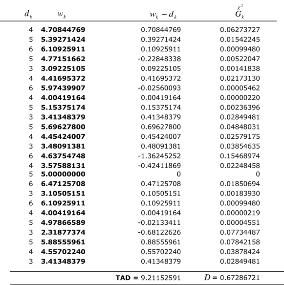
Table 3 New weights and its distance measures to sampling design weights k

d

w

_k

w

_k



d

_k 2  k

G

Now using this result in equation (5), the new weights or calibrated weights for the Chi-squared distance measure can be easily obtained. The calculated new weights and its distance measures to the sample design weights are given in Table 3. For the 16th unit of our hypothetical data, the new weight remains unchanged to the sampling design weight due to the fact that all entries for this unit are zero. However this is very rare in GREGWT reweighting.

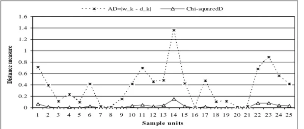
In addition, the total absolute distance (TAD) indicates higher quantity. While absolute distance

has a higher value, the corresponding Chi-squared distance measure also indicates a higher value. However the fluctuations within absolute distances are remarkable compared to Chi-squared distance measures (see in Figure 2).

Furthermore, when the TAD will zero the total Chi-squared distance will also be zero, and in that situation the calibrated weights will remain same as the sampling design weights which indicates the sample data are fully representative to the small area population. Moreover, it is interesting to note that the values of a set of new weights

vary greatly with the changing values of vector for

differences between ^tx,s and Tx. These differences

can come from the poorly representative data and/or the chosen benchmarks. Four random alternative cases of difference vectors

C 1 = [4,3,1,–6,1]‟ , C 2 = [8,3,1,–6,1]‟ , C 3 = [12,3,1, –6,1]‟ and C 4 = [4,3,1,2,1]‟ , where Cj=[Tx– ^tx,s] for j = 1,2,3,4 ,

have been considered and the resulting sets of new weights are plotted in Figure 3. The results show that the case C4 generates a more consistent set of new weights compared to the other cases. It is obvious that when the auxiliary information matrix provides quite rich sample data then the resulting difference vector between ^tx,s

and Tx will be fairly close. Hence the resulting set

of calibrated weights will produce more accurate estimates. 4 4.70844769 0.70844769 0.06273727 5 5.39271424 0.39271424 0.01542245 6 6.10925911 0.10925911 0.00099480 5 4.77151662 -0.22848338 0.00522047 3 3.09225105 0.09225105 0.00141838 4 4.41695372 0.41695372 0.02173130 6 5.97439907 -0.02560093 0.00005462 4 4.00419164 0.00419164 0.00000220 5 5.15375174 0.15375174 0.00236396 3 3.41348379 0.41348379 0.02849481 5 5.69627800 0.69627800 0.04848031 4 4.45424007 0.45424007 0.02579175 3 3.48091381 0.48091381 0.03854635 6 4.63754748 -1.36245252 0.15468974 4 3.57588131 -0.42411869 0.02248458 5 5.00000000 0 0 6 6.47125708 0.47125708 0.01850694 3 3.10505151 0.10505151 0.00183930 6 6.10925911 0.10925911 0.00099480 4 4.00419164 0.00419164 0.00000219 5 4.97866589 -0.02133411 0.00004551 3 2.31877374 -0.68122626 0.07734487 5 5.88555961 0.88555961 0.07842158 4 4.55702240 0.55702240 0.03878424 3 3.41348379 0.41348379 0.02849481 TAD = 9.21152591

D

= 0.67286721

RAHMAN, HARDING, TANTON AND LIU Methodological issues in spatial microsimulation modelling 12

Figure 2 A comparison of absolute distance and Chi-squared distance measures

Figure 3 Plots of sampling design weights and new weights for specific cases

3.3 Combinatorial optimisation reweighting approach

The combinatorial optimisation (CO) reweighting approach was first suggested in Williamson et al. (1998) as a new approach to create synthetic micro-populations for small domains. This reweighting method is mainly motivated towards selecting an appropriate combination of households from survey data to attain the known benchmark constraints at small area levels using an optimization tool. In the combinatorial optimisation algorithms, an iterative process begins with an initial set of households randomly selected from the survey data, to see the fit to the known benchmark constraints for each small domain. Then a random household from the initial set of combinations is replaced by a randomly chosen new household from the remaining survey data to assess whether there is an improvement of fit. The iterative process continues until an appropriate combination of households that best fits known small area benchmarks is achieved (Williamson et al., 1998; Voas and Williamson, 2000; Huang and Williamson, 2001; Tanton et al., 2007). The overall process involves five steps which are as follows:

1. collect a sample survey microdata file (such as CURFs in Australia) and small area benchmark constraints (for example, from census or administrative records);

2. select a set of households randomly from the survey sample which will act as an initial combination of households from a small area; 3. tabulate selected households and calculate total absolute difference from the known small area constraints;

4. choose one of the selected households randomly and replace it with a new household drawn at random from the survey sample, and then follow step 3 for the new set of households combination; and

5. repeat step 4 until no further reduction in total absolute difference is possible.

Note that when an array based survey data set contains a finite number of households it is possible to calculate all possible combinations of households. In theory, it may also be possible to find the set of households‟ combination that best fits the known small area benchmarks. But, in practice, it is almost unachievable, due to computing constraints for a very large number of all possible solutions. For example, to select an

0 0.2 0.4 0.6 0.8 1 1.2 1.4 1.6 1 2 3 4 5 6 7 8 9 10 11 12 13 14 15 16 17 18 19 20 21 22 23 24 25 S am pl e u n i ts D is ta nc e m ea su re AD=|w_k - d_k| Chi-squaredD 0 1 2 3 4 5 6 7 8 1 2 3 4 5 6 7 8 9 10 11 12 13 14 15 16 17 18 19 20 21 22 23 24 25 S am pl e u n i ts We ig h ts d_k w_(C1) w_k(C2) w_k(C3) w_k(C4)

appropriate combination of households for a small area with 150 households from a survey sample of 215789 households, the number of possible solutions greatly exceeds a billion (Williamson et al., 1998).

To overcome this difficulty, the combinatorial optimisation approach uses several ways of performing „intelligent searching‟, effectively reducing the number of possible solutions. Williamson et al. (1998) provide a detailed discussion about three intelligent searching techniques: hill climbing, simulated annealing and genetic algorithms. Later on, to improve the accuracy and consistency of outputs, Voas and Williamson (2000) developed a „sequential fitting procedure‟, which can satisfy a level of minimum acceptable fit for every table used to constrain the selection of households from the survey sample data. The following section will address the simulated annealing method only.

The simulated annealing method in CO

Simulated annealing, an intelligent searching technique for optimisation problems, has been successfully used in the CO reweighting process to create spatial microdata. The method is based on a physical process of annealing – in which a solid material is first melted in a heat bath by increasing the temperature to a maximum value at which point all particles of the solid have high energies and the freedom to randomly arrange themselves in the liquid phase. The process is then followed by a cooling phase, in which the temperature of the heat bath is slowly lowered. When the maximum temperature is sufficiently high and the cooling is carried out sufficiently slowly then all the particles of the material eventually arrange themselves in a state of high density and minimum energy. Simulated annealing has been used in various combinatorial optimisation problems (Kirkpatrick et al., 1983; van Laarhoven and Aarts, 1987; Williamson et al., 1998; Pham and Karaboga, 2000; Ballas, 2001). The simulated annealing algorithm used in the CO reweighting approach was originally based on the Metropolis algorithm, which had been proposed by Metropolis et al. (1953). To simulate the evaluation to „thermal equilibrium‟ of a solid for a fixed value of the temperature

T

the authors

introduced an iterative method, which generates sequences of states of the solid in the following way. As mentioned in the book Simulated Annealing: Theory and Applications by van Laarhoven and Aarts (1987, p. 8):

“Given the current state of the solid, characterized by the position of its particles, a small, randomly generated, perturbation is applied by a small displacement of a randomly chosen particle. If the difference in energy,



E

, between the current state and the slightly perturbed one is negative, that is, if the perturbation results in a lower energy for the solid, then the process is continued with the new state. If

E



0

, then the probability of acceptance of the perturbed state is given by



E KBT



exp . This acceptance rule for new

states is referred to as the Metropolis Criterion. Following this criterion, the system eventually evolves into thermal equilibrium, that is, after a large number of perturbations, using the aforementioned acceptance criterion, the probability distribution of the states approaches the Boltzmann distribution, given as      _    T K E T c E p B exp ) ( 1 ) (

where c(T) is a normalizing factor depending on the temperature T and KB is the Boltzmann constant.” To search an appropriate combination of households from a survey dataset that best fits the benchmark constraints at small area levels is a combinatorial optimisation problem, and solutions in a combinatorial optimisation problem are equivalent to states of a physical annealing process. In the process of CO reweighting by simulated annealing algorithm, a combination of households takes the role of the states of a solid while the total absolute distance (TAD) function and the control parameter (for example, rate of reduction) take the roles of energy and temperature respectively. According to Williamson et al. (1998), change in energy becomes potential change in households‟ combination performance (assessed by TAD) to meet the benchmarks, and temperature becomes a control for the maximum level of performance degradation (% of reduction) acceptable for the change of one element in a combination of households by a random element picks from the sample data. The control parameter is then lowered in steps, with the system being allowed to approach equilibrium for each step by generating a sequence of combinations by obeying the Metropolis criterion.

In addition, the algorithm is terminated for some small value of the control parameter, for which practically no deteriorations are accepted. Hence the normalizing constant which is depending on the controlling factor as well as Boltzmann constant can be dropped from the probability distribution. In this particular case we have the equation:

.

exp

)

(











 

_





T

E

E

p

There are two important features of this probability equation described by Williamson et al. (1998). One is that the smaller the value of difference in energy, E, the greater is the

likelihood of a potential replacement being made in a combination. Another feature is that the smaller the value of controlling factor T, the smaller the change in performance likely to be accepted.

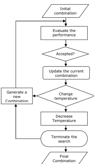
A typical simulated annealing algorithm is depicted in Figure 4. The overall process consists of a series of iterations in which random shifting is occurring from an existing solution to a new solution among all possible solutions. To accept a new solution as the base solution for further iteration, a test of goodness-of-fit based on TAD is consistently

RAHMAN, HARDING, TANTON AND LIU Methodological issues in spatial microsimulation modelling 14 checked. The rules of the test are if the change of

the difference in energy is negative, the newly simulated solution is accepted unconditionally; otherwise it is accepted satisfying the abovementioned Metropolis criterion. The simulated annealing algorithm may be able to avoid deceiving at local extremum in the solutions. Moreover, a solution or selected combination of households by this algorithm can generate real individuals living in actual households in a sense that individuals are from modelled outputs and not synthetically reconstructed (Ballas, 2001).

Figure 4 A flowchart of the simulated annealing algorithm

(after Pham and Karaboga, 2000)

An illustration of CO process for hypothetical data

A simplified combinatorial optimisation process is depicted in Figure 5. It is noted that in this process when the total absolute difference (aforementioned TAD) in gregwt section) is equal to zero, the selection of households‟ combination indicates the best fit. In other words, in this case the new weights give the actual households units from the survey sample microdata, which are the best representative combination. Thus it is a selection process of an appropriate combination of sample units, rather than calibrating the sampling design weights to a set of new weights.

4. COMPARISON OF REWEIGHTING

TECHNIQUES AND A NEW APPROACH In this section, a comparison of the two reweighting methodologies is given with a new approach to the creation of synthetic spatial microdata.

4.1 Comparison of GREGWT and CO

Although both the reweighting approaches are widely used in the creation of small area synthetic microdata, the methodology behind each approach is quite different. For instance, GREGWT is typically based on generalised linear regression and attempts to minimize a truncated Chi-squared distance function subject to the small area benchmarks. Combinatorial optimisation, on the other hand, is based on „intelligent searching‟ techniques and attempts to select a combination of appropriate households from a sample that best fits the benchmarks.

Tanton et al. (2007) provide a comparison of these two approaches using a range of performance criteria. The study also covers the advantages and disadvantages of each method. Using the data of the 1998-99 Household Expenditure Survey from Australia, the study reveals that the GREGWT algorithm seems to be capable of producing good results. However the GREGWT algorithm has some limitations compared to the combinatorial optimisation algorithm. One of the drawbacks of GREGWT approach is that for some small areas, „convergence‟ does not exist. That means that the GREGWT algorithm is unable to produce estimates for those small areas, while the combinatorial optimisation algorithm is able to do so. In addition, the GREGWT algorithm takes more time to run compared to combinatorial optimisation, and it is still unclear whether that extra time is due to the different programming language (GREGWT is written in SAS code and CO uses compiled FORTRAN code) or the relative efficiencies of the underlying algorithms. Moreover the combinatorial optimisation routine has a tendency to include fewer households but give them higher weights – and, conversely, the GREGWT routine has a tendency to select more households but give them smaller weights.

A comparison of the GREGWT and CO reweighting approaches is summarized in Table 4. The focus is here mostly on methodological issues. However some entries are consistent with Tanton et al. (2007). Generate a new Combination Evaluate the performance Initial combination Accepted? Decrease Temperature Update the current

combination Change temperature Terminate the search Final Combination

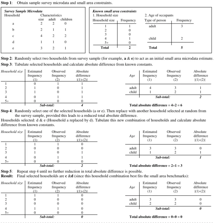
Figure 5 A simplified combinatorial optimisation process Step 1: Obtain sample survey microdata and small area constraints.

Step 2: Randomly select two households from survey sample (for example, a & e) to act as an initial small area microdata estimate.

Step 3: Tabulate selected households and calculate absolute difference from known constants.

Household size Estimated Observed Absolute Estimated Observed Absolute frequency frequency difference Age frequency frequency difference

(1) (2) |(1)-(2)| (1) (2) |(1)-(2)| 1 0 1 1 2 1 0 1 adult 4 3 1 3 1 0 1 child 1 2 1 4 0 1 1 Sub-total: 2 5+ 0 0 0

Sub-total: 4 Total absolute difference = 4+2 = 6

Step 4: Randomly select one of the selected households (a or e). Then replace with another household selected at random from the survey sample, provided this leads to a reduced total absolute difference.

Households selected: d & e (Household a replaced by d). Tabulate this new combination of households and calculate absolute difference from known constants.

Household size Estimated Observed Absolute Estimated Observed Absolute frequency frequency difference Age frequency frequency difference

(1) (2) |(1)-(2)| (1) (2) |(1)-(2)| 1 1 1 0 2 0 0 0 adult 3 3 0 3 1 0 1 child 1 2 1 4 0 1 1 Sub-total: 1 5+ 0 0 0

Sub-total: 2 Total absolute difference = 2+1 = 3

Step 5: Repeat step 4 until no further reduction in total absolute difference is possible.

Result: Final selected households are c &d (since this household combination best fits the small area benchmarks):

Household size Estimated Observed Absolute Estimated Observed Absolute frequency frequency difference Age frequency frequency difference

(1) (2) |(1)-(2)| (1) (2) |(1)-(2)| 1 1 1 0 2 0 0 0 adult 3 3 0 3 0 0 0 child 2 2 0 4 1 1 0 Sub-total: 0 5+ 0 0 0

Sub-total: 0 Total absolute difference = 0+0 = 0

(after Huang and Williamson, 2001)

Known small area constraints

1. Household size 2. Age of occupants

Household size Frequency Type of person Frequency 1 1 adult 3 2 0 3 0 4 1 child 2 5+ 0 Total 2 Total 5

Survey Sample Microdata

Household Characteristics size adult children a 2 2 0 b 2 1 1 c 4 2 2 d 1 1 0 e 3 2 1

RAHMAN, HARDING, TANTON AND LIU Methodological issues in spatial microsimulation modelling 16 Table 4 A comparison of the GREGWT and CO reweighting methodologies

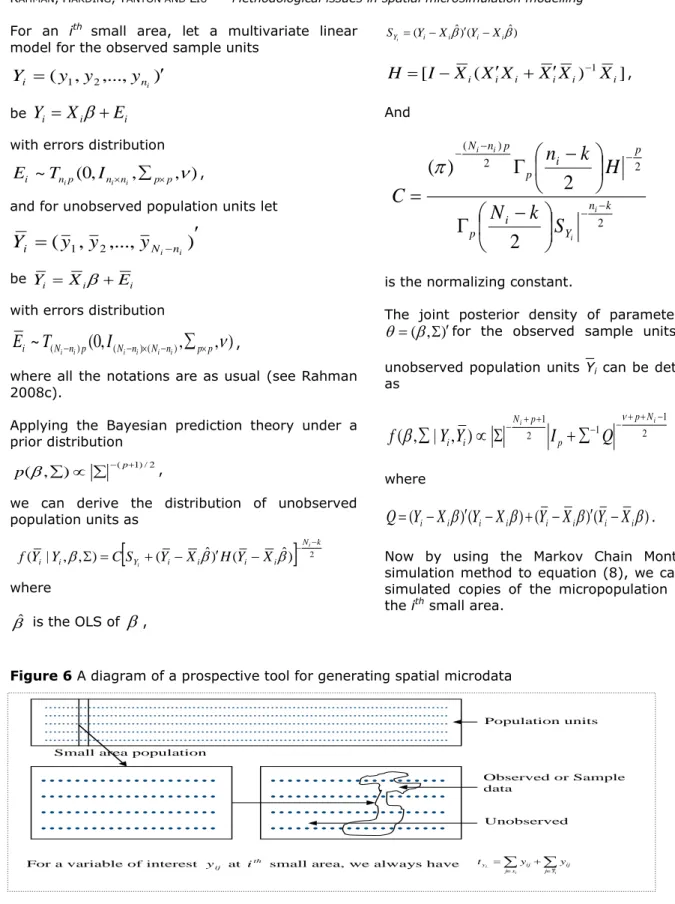
4.2 Bayesian prediction approach of small area microdata simulation

A new system for creating synthetic spatial microdata is offered in this subsection. It is noted that after the sample survey, a finite population usually has two parts - which are observed units in the sample called data and unobserved sampling units in the population (Figure 6). Suppose Ω represents a finite population in which Ωi (say) is

the subpopulation of small area i. Now if si

denotes the observed sample units in the ith _area

then we have

si

s

_

i= Ωi Ω for i,

where

_

s

i denotes the unobserved units in the

small area population. Let yij represents a variable

of interest for the jth _{characteristic of the}

population at ith _{small area. Thus we always have}

the estimate of population total at ith _{small area}





 





i i i s j j s ij ij y

y

y

t

. .

The main challenge in this process is to establish the link of observed data to the unobserved sampling units in the population. It is a kind of prediction problem, where a modeller tries to find

a probability distribution of unobserved responses using the observed sample and the auxiliary data. The Bayesian methodology (see Ericson, 1969; Lo, 1986; Little, 2007; Rahman, 2008b) can deal with such a prediction problem.

The Bayesian prediction theory is very straightforward and mainly based on the Bayes‟s posterior distribution of unknown parameters (Rahman 2008c). Let y be a set of observed units from a model with a joint probability density

p(y|), in which  is a set of model parameters. If a prior density of unknown parameters  is g, the posterior density of  for given y can be obtained by Bayes‟s theorem and defined as p(y|) p(y|)

g().

Now, if

_

y

is the set of unobserved units in a finite population, then under the Bayesian methodology its prediction distribution can be obtained by solving the integral







p



y

p

y



d



y

y

p

(

|

)

(

|

)

(

|

)

,

where p(

_

y

|

) is the probability density of unobserved units. Details of the Bayesian prediction theory for various regression models are given in Rahman (2008c).

GREGWT CO

o An iterative process. o An iterative process.

o Use the Newton-Raphson method of iteration. o Use a stochastic approach of iteration MCMC. o Based on a distance function. o Based on a combination of households.

o Attempt to minimize the distance function subject to the known benchmarks. o

Attempt to select an appropriate combination that best fits the known benchmarks.

o Use the Lagrange multipliers as minimisation tools for minimising the distance function. o

Use different techniques as intelligent searching tools in optimizing combinations of households. o Weights are in fractions. o Weights are in integers (but could be fractions). o Boundary condition is applied to new weights

for achieving a solution. o There is no boundary condition to new weights. o The benchmark constraints at small area levels

are fixed for the algorithms. o

The algorithm is designed to optimize fit to a selected group of tables, which may or may not be the most appropriate ones. Hence there may be a choice of benchmark constraints.

o Typically focus on simulating microdata at small area levels and aggregation is possible at larger domains.

o Offers a flexibility and collective coherence of microdata, making it possible to perform mutually consistent analysis at any level of aggregation or sophistication.

o All estimates have their own standard errors

obtained by a group jackknife approach. o No information about this in literature. May be possible in theory but nothing available in practice.

o In some cases convergence does not exist and this requires readjusting the boundary limits or a proxy indicator for this nonconvergence.

o There are no convergence issues. However, the finally selected household combination may still fail to fit user-specified benchmark constraints. o There is no standard index to check the

statistical reliability of the estimates. o There is no standard index to check the statistical reliability of the estimates. o The iteration procedure can be unstable near a