This is an author produced version of A route-swapping dynamical system and Lyapunov function for stochastic user equilibrium.
White Rose Research Online URL for this paper: http://eprints.whiterose.ac.uk/93130/
Article:
Smith, MJ and Watling, DP (2016) A route-swapping dynamical system and Lyapunov function for stochastic user equilibrium. Transportation Research Part B: Methodological, 85. pp. 132-141. ISSN 0191-2615
https://doi.org/10.1016/j.trb.2015.12.015
© 2016, Elsevier. Licensed under the Creative Commons Attribution-NonCommercial-NoDerivatives 4.0 International http://creativecommons.org/licenses/by-nc-nd/4.0/
promoting access to White Rose research papers
[email protected] http://eprints.whiterose.ac.uk/
1
A ROUTE-SWAPPING DYNAMICAL SYSTEM AND LYAPUNOV FUNCTION
FOR STOCHASTIC USER EQUILIBRIUMMichael J. Smith (Department of Mathematics, University of York) David P. Watling (Institute for Transport Studies, University of Leeds)
Abstract An analysis of the continuous-time dynamics of a route-swap adjustment process is presented, which is a natural adaptation of that which was presented in Smith (1984) for deterministic choice problems, for a case in which drivers are assumed to make perceptual errors in their evaluations of travel cost, according to a Random Utility Model. We show that stationary points of this system are stochastic user equilibria. A Lyapnuov function is developed for this system under the assumption of monotone, continuously differentiable and bounded cost-flow functions and a logit-based decision rule, establishing convergence and stability of trajectories of such a dynamical system with respect to a stochastic user equilibrium solution.
1. INTRODUCTION
There is now a growing body of literature examining the kinds of smooth, continuous-time trajectories which might approximate the day-to-day dynamic adjustment processes of car drivers in transport networks. These begin by postulating a continuously-varying state variable (e.g. representing network flows, costs or cost differences) together with some autonomous, continuous-time dynamical system:
(1)
for some given, smooth, time-independent function f : n, where n, and the function x : [0,) is differentiable at all times t > 0. Typically in such systems, we begin with specifying the form of f, and then the following initial value problem is of interest: given some , find a function x(.) which is continuous at t = 0, differentiable at t > 0, differentiable on the right at t = 0, and solves the system of equations:
With such dynamical systems, it is natural to explore the properties of fixed/stationary point equilibria of the system, namely those x satisfying:
and then to ask of such point equilibria: which ones are likely to emerge and persist as the convergent behaviour of system (1), i.e. which equilibria are stable ?
Papers that have explored various dynamical route adjustment processes of the form (1) include those by Smith (1984), Friesz et al. (1994), Zhang and Nagurney (1996), Zhang et al. (2001), Yang and Liu (2007), Yang and Zhang (2009), He et al. (2010), Han and Du
(2012), Guo et al. (2013) and Zhang et al. (2015). All of these established the Wardrop Deterministic User Equilibrium (DUE) state as a fixed point of their dynamical system. A subset of these also established general conditions to ensure global asymptotic stability of the Wardrop equilibrium solution with respect to the particular dynamical system they specified; notably Smith (1984); Friesz et al. (1994); Zhang and Nagurney (1996); and Han and Du (2012). Yang and Zhang (2009) established that many of these rerouting dynamics are special cases of a general dynamic, which they termed a Rational Behavior Adjustment Process. However, as Zhang et al. (2015) recently noted, the
process proposed originally by Smith is in some respects the most natural and
has the simplest formulation and has stimulated various extensional applications. This process, which has subsequently been termed the Proportional-Switch Adjustment Process or simply the Smith dynamic (Sandholm, 2010), is an important reference case for the present paper.
Several authors have also considered dynamical route adjustment processes for which the fixed points coincide with the Stochastic User Equilibrium (SUE) model. Horowitz (1984) studied the convergence properties of a variety of discrete-time decision rules for two-route networks. Cantarella and Cascetta (1995) considered a very wide class of discrete-time dynamic processes, but also established specific results for a particular process in which (a) a fixed proportion (0< 1) of travellers reconsider their
previous day s choice and b forecasted path costs are based on a convex combination
of the latest experience (with weight 0< 1) and the previous forecast. They showed that, under typically-assumed conditions, small enough values of and exist to ensure stability of SUE with respect to such a system. Watling (1999) considered a special case of such a process, with = 1, and set out sufficient conditions on to ensure stability, which through a route re-labelling strategy were shown to be applicable to a quite wide class of such problems. In addition, relationships were explored between stability/instability properties in discrete and continuous time, which were further explored by Cantarella and Watling (2015). The continuous-time model explored in Watling (1999) is a second important reference-case for the present paper, being what Sandholm (2010) subsequently termed the logit dynamic. In addition, Watling presented methods for estimating domains of attraction for multiple equilibria, which were further refined and elaborated by Bie and Lo (2010). Yang and Liu (2007) established that various existing processes could be viewed as the mean dynamic of a stochastic process, mainly focusing on dynamical systems related to DUE, but also presented numerical experiments for the logit dynamic and its relation to SUE. Guo et al (2013, Appendix B), while mainly concerned with DUE, established convergence for a discrete-time form of the logit dynamic.
The purpose of the present paper is to formulate and analyse a new form of dynamical system for SUE, differing from the logit dynamic and developed from the logic of the Smith dynamic proposed for DUE. In doing so, we provide a kind of bridge between DUE- and SUE-based dynamical modelling, in the sense that the dynamic processes of the two are connected, not only the equilibrium states. We achieve this by developing a route-swapping dynamical system and a corresponding Lyapunov function, which can be seen to be the SUE analogue of the dynamical process and results presented in Smith (1984) for DUE.
3 2. BASIC STATIC NOTATION
We suppose that our network consists of k origin-destination (OD) movements with positive demands contained in the vector q of length k. Consider the finite set of all routes that visit no link twice, across all OD movements, and suppose that there are n such routes in total. Let the matrix A denote the (OD-movement)-route incidence matrix, of dimension k n, any element of which is 1 if the route serves the given OD movement and 0 otherwise. We may then define the convex set of demand-feasible route flows as:
�ith and
where x has the elements denoting the steady flow along route r for . In addition, we define the set of n-dimensional vectors in Euclidean space with strictly positive elements as:
�ith for .
Let be the given route costflow function, such that is the cost of travelling on route r when the route flow vector is x (for r n). We suppose that c(x) is a monotone, continuously differentiable function of defined throughout D.
3. DEVELOPMENT OF A RUM-BASED, ROUTE-SWAPPING DYNAMIC
Since it was originally proposed in Smith (1984), the pairwise route-swapping dynamic has emerged as a standard reference model in the evolutionary game theory literature, where it is referred to as the Smith dynamic (Sandholm, 2010). The key behavioural aspects of this dynamic are: (a) pairwise path-swapping from more costly to less costly paths; and (b) for those pairs of paths in (a), an assumed rate of exchange of path flow proportional to the product of the path flow on the higher cost path and the cost surplus of the higher over the lower cost path. A limitation of this model, however, is that it does not allow for possible mis-perceptions of travellers in their evaluations of travel costs. Here, we aim to modify the Smith dynamic to incorporate mis-perception as represented by a Random Utility Model (RUM), while aiming to retain as much as possible of the originally-proposed behavioural process. In particular we assume pairwise path-swapping from less attractive to more attractive routes, but depart from the original
model in how the attractiveness is defined
Consider a pair of paths (r, s) serving the same origin-destination (OD) movement at time t, with current flows xr(t) and xs(t and current measured travel costs cr(x(t)) and
cs(x(t)). Suppose that traveller mis-perception is modelled by a multinomial logit model
with dispersion parameter 1. Suppose that we are an observer of this OD movement,
then if we randomly selected a traveller making this movement, the current relative odds of that traveller being a path r rather than path s traveller would clearly be given by the ratio . If, on the other hand, travellers were able to immediately
readjust their route choice in response to the prevailing travel costs, then according to the multinomial logit model, these relative odds would be
exp exp . The difference between these two cases (the current flows and the immediately readjusted flows) can be measured by the odds ratio:
exp
exp
(Note that since we are supposing that cr(x) is a continuously differentiable function of x
throughout S, then so is also a continuously differentiable function of x throughout S.) An odds ratio of would denote that the split of traffic between the two paths was exactly in accordance with the prevailing travel costs, according to a multinomial logit model, whereas indicates that path r has too much flow relative to path s, according to the prevailing travel costs. Therefore, at the aggregate OD level, the odds ratio can be used as the basis for suggesting an overall route-swapping dynamic for the population of travellers using that movement.
It should be noted that we do not suggest individual travellers perceive such a stimulus; rather we use an aggregate but probabilistically distributed model, with the random utility model applied to suggest the overall effect on the population of travellers for that movement. It is also noted that the Independence from Irrelevant Alternatives (IIA) property of the multinomial logit model means that it makes sense to make such pairwise comparisons as implied by (2), since under this RUM the flow-split between any pair of alternatives does not depend on the costs of other alternatives. In order to develop this dynamic in combination with something close to the original Smith dynamic constructed for deterministic choice models, it is natural to transform the odds ratio so that a stimulus level of zero suggests no flow-swap is needed, and a positive value suggests a flow swap is needed away from route r to route s.
In order to do so, a scalar function is defined, such that:
h is continuously differentiable and monotonically increasing on the open interval (0,); and
.
This scalar function is used to transform the odds ratio (2) for use in a route-swapping system, according to:
(3)
with (2) and (3) then used to define the system:
(4) where is given by:
5
for all
where for any real number y
max
and where rs is a path-swap indicator vector of dimension n. This latter vector is the
zero vector if routes r and s serve different OD movements or if r = s; otherwise, it has 1 for the rth element, +1 for the sth element, and zeroes elsewhere. The sets and were
defined in section 2.
Equations (2) (5) define a family of dynamical systems; a particular instance of this family corresponds to a particular choice of the function h(.) (satisfying the required conditions on h). We shall initially consider the two possibilities:
(6)
or
ln . (7)
Both of (6) and (7) satisfy the required conditions on h, and both contain a free
parameter allowing the rate of adjustment of the process to be tuned independently of
the equilibrium properties.
While both (6) and (7) give rise to candidate dynamical systems that can be related to SUE, we propose that (7) has two key advantages:
Firstly, when (7) is combined with (2)/(3), it implies that the path-swapping is governed by the log-odds ratio ln , a commonly-used measure in statistics (e.g. Cramer, 2003; Hilbe, 2009). In that field, the logarithm is favoured over the direct use of the odds-ratio for a reason that also has relevance in our present context. Namely, directly using the odds-ratio as in (6) has a disadvantage that the scale of the implied stimulus is asymmetric in its implied sensitivity. For example, if , ,
exp , exp , then using the linear function
(6) we find ; on the other hand, reversing the roles of routes r and s, the reverse stimulus is much smaller in magnitude, with
. Adopting the logarithmic transform (7), on the other hand, the magnitude of the dynamic stimulus is insensitive to the route labelling, with
ln .
Secondly, the logarithmic transform (7) provides a direct link to the original Smith dynamic for DUE, as a limiting case. In order to see this, we note that (7) combined with (2)/(3) is readily simplified to:
ln and setting ( , this may be re-written as:
ln . (8)
In comparison, in the DUE case, we consider a slight generalisation of the Smith dynamic, in which the rate of change in route flows is a constant multiplied by the original Smith dynamic (i.e. the original Smith dynamic for DUE corresponds to the choice ). This generalised Smith dynamic can then be expressed as the system (4) and (5) in combination with the choice:
. (9)
Although is not permitted in our RUM-based dynamical system, it is clear from (8) and (9) that for small values of the dynamic implied by (8), will approximate that implied by (9). Although (9) may be interpreted either as an individual stimulus for travellers to change or as an aggregate OD-level stimulus, the dynamic implied by (8) only has an aggregate OD level interpretation, since the additional term is expressing the rate of adjustment of the population of travellers on that OD movement, given the assumptions about the distribution of perception errors across this population (as contained in ).
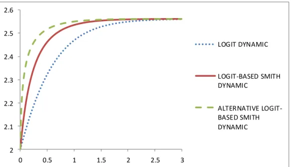
As we shall exemplify with an example, the dynamical systems implied by (6) or (7) (in combination with (2) (5)) are new ones, and in particular, they differ from the logit dynamic previously studied in the literature (as discussed in section 1). In order to illustrate this, consider a simple example of a single OD movement with a demand of served by two parallel routes, with route cost functions and
. Suppose the logit parameter , that the parameters in (6) and (7) are given by and , and suppose the initial conditions of the system are . We refer to the system implied by equations (2) (5) with (7) as the logit-based Smith dynamic, and the system implied by equations (2) (6) as the alternative logit-based Smith dynamic. Figure 1 illustrates the trajectory of the flow on route 1 as a function of time (horizontal axis), for each of these dynamical systems. We can see that even for an example with only two routes, the three systems differ; i.e. they do not differ simply because of the pairwise way in which (5) is constructed, since in this small example this is not a relevant distinction. All three provide smooth trajectories that, at least for the initial condition and example network tested, converge to SUE. Although neither individual nor aggregate behaviour in real-life systems can be expected to be smooth in this way, the three models are all viable candidates as smooth approximations to the underlying real-life system, but with different rates of system
7
adjustment. Based on the nature of the observed flow adjustments over time, and in particular the manner in which they approach something akin to equilibrium, one such model could be chosen as a best approximation to the real-life system.
2 2.1 2.2 2.3 2.4 2.5 2.6 0 0.5 1 1.5 2 2.5 3 LOGIT DYNAMIC LOGIT-BASED SMITH DYNAMIC
ALTER NATIVE LOGIT-BASED SMITH DYNAMIC
Figure 1: Route 1 flow as a function of time for three alternative logit-related dynamical systems
In the present paper, for the reasons already explained above, we shall henceforth focus on the logit-based Smith dynamic, which as we noted above can be expressed by the system (4)/(5)/(8). In doing so, we provide evidence on the theoretical properties of a new candidate model, which can be considered alongside existing results for the logit dynamic. As noted above the model then has the attractive feature that it provides a bridge to the seminal work with DUE on the Smith dynamic, which the logit-based Smith
dynamic approaches as the assumed variance in travellers perceptual errors as
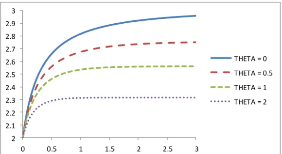
controlled by ) approaches zero. Figure 2 illustrates this for the two-route example network considered earlier (for = 1). That is to say, it is not simply that as , there is a limit point that approaches DUE, but that also the trajectory of the dynamical adjustment process towards equilibrium for the logit case approaches the deterministic one (labelled as
2 2.1 2.2 2.3 2.4 2.5 2.6 2.7 2.8 2.9 3 0 0.5 1 1.5 2 2.5 3 THETA = 0 THETA = 0.5 THETA = 1 THETA = 2
Figure 2: Route 1 flow as a function of time for three cases of the Logit-based Smith Dynamic, and (for 'THETA= 0') the original Smith Dynamic
4. THEORETICAL ANALYSIS OF THE LOGIT-BASED SMITH DYNAMIC
In the present section we establish a series of theoretical results concerning the Logit-based Smith Dynamic given by (2) (5) with (7), which we showed in the previous section to be expressible in an equivalent form (4)/(5)/(8) which is re-stated below to avoid any ambiguity. Since the case = 1 provides the direct generalisation of the original Smith dynamic for DUE (and since the results are anyway trivially extended for any > 0), we shall restrict attention to the case = 1. The system is then:
(10)
for all
ln for all (12) where all other relevant notation was defined in section 2. We note that under the assumptions stated in section 2, each given in (12) is a continuously differentiable function of x in S since we are assuming that each is a continuously differentiable function of x in S. It further follows that given by (11), when combined with (12), is a Lipschitz continuous function of x on any compact subset of S. (Continuous
differentiability is lost due to the suffix in the term ; but Lipschitz
continuity remains.)
We begin, in Lemma 1, by formally establishing the relationship of this dynamical system with the Stochastic User Equilibrium (SUE) model (Sheffi, 1985).
9 Lemma 1
If is an SUE, then it is a point equilibrium of system (10) (12). Further if is an equilibrium point of (10) (12), then it is an SUE.
Proof
By the Independence from Irrelevant Alternatives property of the multinomial logit model, a necessary and sufficient condition for logit SUE is that and for any pair of routes (r, s) serving the same OD movement:
exp
exp
This condition holds (according to (12)) if and only if
for all such that Hence:
thus establishing the if part of the Lemma.
Conversely, suppose and that it is an equilibrium point of (10) (12). Then,
Now put
ln so that
Projecting this zero vector onto
It follows that
Each term is non-negative and so there is no cancellation. It follows (since the sum of these terms is zero) that each term is zero and hence
for all r, s such r~s. Consider any (r, s) on the same OD movement, written as r ~ s. Then since x S by hypothesis, all components of this vector xr > 0, and so it follows from the
above that for all such route pairs r ~ s:
ln
It follows that x is an SUE (noting the necessary and sufficient condition for SUE stated
at the start of the if part of this proof and so we have proven the only if part of the
result. .
We note that it is known that if the cost function c is continuous and monotone on D then there exists a unique SUE solution e in (Cantarella and Cascetta, 1995). These properties of existence and uniqueness will be exploited in our subsequent results. We now explore the dynamics of system (10) (12) through a series of results. These results in turn show that (for monotone, continuously differentiable c(.)):
(i) a (smooth) locally unique solution trajectory exists to differential equation (10) (12) (Lemma 2);
(ii) a Lyapunov function V may be constructed on (Lemma 3); (iii) any solution trajectory stays away from the boundary of (Lemma 4);
(iv) solution trajectories of (10) (12), in staying away from the boundary of S, may be defined for all t 0 thus, for example, no solution trajectory is prematurely terminated by hitting the boundary of S (Lemma 5 and Corollary 1); and
(v) a convergence/stability result on system (10) (12), in relation to SUE, may then finally be established (Theorem 1).
Lemma 2
Let c be continuously differentiable1 on and let Then there exists
> 0 and a unique solution to (10) (12) for Proof
Let . Now c is a continuously differentiable function of x throughout So there is r(x0) > 0 such that is defined and Lipschitz continuous throughout the closed
neighbourhood clB(x0, r(x0)) of x0 )t follows from Picard s theorem (see appendix A)
that there is and exactly one solution of (10) (12) defined for all
Moreover:
1 Continuous differentiability is unnecessarily strong but since it is assumed in a later
11
(14)
thus establishing the result.
Discussion
Suppose in this discussion that the conditions stated in Lemma 2 hold. Then Lemma 2 ensures that for each x0 there is a positi�e such that there exists a unique
solution x(.) to (10)(12) defined on the time interval given by (14) (and therefore on the interval [0, ]). Now, we wish to show that this unique solution x(.) to (10)(12) can be extended from the time interval to the time interval (or from [0 ] to ); so that the solution is uniquely defined for all future time.
Suppose now that we apply Lemma 2 for various , and make the further key assumption that the which arise may be chosen (for all relevant ; those which arise) to be independent of x0; let this be denoted Under this key assumption, we
may now use Picards theorem successively at our particular initial x0, then at x( , then at x( ), then at x( , etc. There must then be (by these successive applications of
Picard s theorem unique continuously differentiable solutions of (10)(12) over each of
the equal-length time intervals:
.
In this case the above successively generated solutions clearly fit together to yield a unique solution defined over the time interval:
which contains . Thus, based on our assumptions, we have proved that there is a unique solution with start point and defined for all future time.
But can such a be chosen to justify our key supposition above? We need to be independent of these relevant (successively generated) initial points (namely the points x0, x , x( ), x( ), . . . . ). To show that this choice is possible we need to utilise a Lyapunov argument for the system (10)(12), as follows.
Lemma 3 (A Lyapunov result when c is monotone) Consider the (scalar) objective function where
ln ln (15)
Suppose the route cost-flow function c(.) is non-negative, continuously differentiable (and so bounded) on D, and monotone on D. (Thus any unboundedness in (15) must arise from the ln terms.) Let Let x(.) be the unique solution of the dynamical system (10)(12) starting at and defined for all
Proof
We begin by noting that it is possible to re-write (12) as:
ln ln
and so we may imagine that drivers are motivated by a deterministic Smith dynamic (Smith, 1984) but with the original route cost function replaced with ln (where ln denotes ln ln ln ). Then, the result is established by applying the proof of descent in Smith (1984, Appendix), but showing in this case that is a descent direction for V whenever belongs to rather than , and for the route cost function ln rather than . This modified result however must hold, since if is monotone on then ln is monotone on .
Lemma 4
Suppose that the conditions stated in Lemma 3 hold and that V is defined by (15). Let M0 > 0 and F = {x ; V(x M0}.
Then there is a constant R > 0 such that
boundary for all
Proof
Let M0 > 0 and F = {x ; V(x M0}. Let x belong to F. Then:
ln ln
for all (r, s) such that r ~ s.
Now, at each x in F, choose a route (joining any OD movement) so as to minimise ln and denote this chosen s by . That is to say:
and ln ln .
If there is a tie for the minimum, then arbitrarily choose one of these routes and call this .
Then for each in having chosen , choose a route r on the same OD movement so as to maximise , and denote this by . That is to say:
and ln ln .
If there is a tie for the maximum on that OD movement, arbitrarily choose one of the routes and call this .
Now, this maximum route flow is certainly bounded below since:
min
where we have defined for the first time above. To see this result, suppose that we chose an OD movement with smallest demand flow (i.e. one with OD demand
13
min ) and then spread traffic evenly across the feasible routes for that movement. Certainly the number of feasible routes for that movement is less than or equal to the total number of routes n, and so certainly this fractional spread must be greater than or equal to , as defined above. Note that since we suppose that every OD movement has a strictly positive flow.
Now from our earlier remark, with and :
ln
ln
and with our bound above on the route flows, it then follows that:
ln ln whence: ln ln and so: ln ln
Since by hypothesis, cr(.) is non-negative and bounded above on (by B, say), it follows
that , and hence:
ln ln
Using once more the bound on the maximum route flow, together with the fact that the ln function is increasing
ln ln
Rearranging:
ln ln
exp ln say
Recalling that, at any fixed x in , the component of is chosen to be the smallest component of x, it follows that the distance between any component of x and the boundary of must exceed this positive constant R.
Corollary 1
Under the conditions of Lemma 4, the local solutions defined for each possible start point x0 fit together to create a solution x(.) starting at any x0 in and
defined for all time t in [0, Proof
This result follows from the previous discussion and Lemma 4. We need to show that we can choose a that is independent of the relevant x. So let x0 belong to , let M0 = V(x0) and let F = {x ; V(x M0}. Although is not closed the set F is closed since
V is continuous. Also F is bounded and so (being both closed and bounded) is compact. Relevant x here are those x in F.
Then by Lemma 4 there is a constant R > 0 such that
boundary for all
Now c is continuously differentiable on and so on
F0 = boundary
Also F0 is (like F ) a closed and bounded set in Euclidean space and so is compact. Hence the derivative of c, being continuous on F0, is also bounded on F0 (which contains F). It follows (as remarked above) that c and hence is Lipschitz continuous on F0 and so also on the subset F. So there exists K > 0 such that
for all x, y
By choice of R above, for all x in F: the closed ball B = cl[BR/2(x)] is a subset of S. It now
follows from Picard s theorem (see Hunter (1996) and appendix A) that if we put
= R/(2M0)
then for each x0 there is a unique solution of (10)(12) defined on [- , where is
not dependent on x0 so long as x0 . Now we know that each trajectory starting in F
stays in F, since V decreases along a trajectory by Lemma 3. Thus, as indicated in the
discussion using Picard s theorem successively at our particular initial x0, then at x( ,
then at x( , then at x , . . . . . , there must be unique solutions of (10)(12) over each of the equal-length time intervals:
.
(Of course, by the Lyapunov result in Lemma 3, x0 implies that x() , which in turn implies that x , which in turn implies that x( . . . . .) The proof is completed.
15 Lemma 5
Under the conditions given in Lemma 3, any solution x(.) of (10)(12) starting at x0 (and so defined for all t , by Lemma 4) satisfies:
V(x(t)) 0 as t Proof
We have shown that no solution trajectory starting at x0 ever leaves F = {x
; V(x V(x0)}. So by Lemma 4 such trajectories run for all time t Then the
proof of the Lyapunov result in Smith (1984) may be applied to show that V(x(t)) 0 as t
Theorem 1
Let e be the unique SUE2. Under the conditions of Lemma 3, given any start point x0 in
, any solution x(.) of (10)(12) starting at x0 must satisfy dist(x(t), e) 0 as t
Proof
By Lemma 5, V(x(t)) 0 as t V is continuous and V(x)= 0 if and only if x = e. Also x(t) belongs to F = {x ; V(x V(x0)} for all t > 0; and F is compact. Therefore
dist(x(t), e) 0 as t 5. CONCLUDING REMARKS
In this paper we have presented a path-swapping, continuous-time dynamical system that is a RUM-based analogue of the system proposed by Smith (1984) for deterministic choice systems. We have established that equilibria of this system are SUE solutions, and have gone on to establish a corresponding Lyapunov-style result for such a system. This work opens up several opportunities for further research, including: i) the possibility to extend existing stability results for SUE in discrete time, which currently require a case-by-case analysis of network properties; ii) possibilities to devise stabilising control and pricing measures that exploit such properties; iii) the connection of the results presented with classes of dynamic process that have been identified for
DUE-related systems such as rational behaviour adjustment processes ; and iv) the
extension of the results to other choice models that may naturally be formulated as pairwise swaps, such as weibit (Castillo et al, 2008) and path-size logit/weibit (Kitthamkesorn and Chen, 2013), as well as more general choice models adopting the kinds of swapping dynamics suggested in Watling (1998).
2 As we remarked earlier, existence and uniqueness of SUE follows from our hypotheses on the cost
Acknowledgements
We would like to thank all three anonymous referees for their very constructive critical comments on earlier drafts of this paper, which helped us to significantly improve the paper.
References
Bie, J. & Lo, H. (2010). Stability and attraction domains of traffic equilibria in a day-to-day dynamical system formulation. Transportation Research 44B, 90 107.
Cantarella, G.E & Cascetta, E. (1995). Dynamic Process and Equilibrium in Transportation Networks: Towards a Unifying Theory. Transportation Science 29, 305-329.
Cantarella, G.E. & Watling, D.P. (2015). Modelling road traffic assignment as a day-to-day dynamic, deterministic process: A unified approach to discrete and continuous time models. EURO Journal of Transportation and Logistics, in press, doi: 10.1007/s13676-014-0073-1.
Castillo, E., Menéndez, J. M., Jiménez, P. and Rivas, A., (2008). Closed form expression for choice probabilities in the Weibull case, Transportation Research Part B, 42(4), 373-380.
Cramer, J. S. (2003). Logit Models from Economics and Other Fields. Cambridge University Press.
Friesz, T.L., Bernstein, D., Mehta, N.J., Tobin R.L., Ganjalizadeh (1994). Day-to-day dynamic network disequilibria and idealized traveller information systems. Operations Research 42(6), 1120 1136.
Guo, R.Y., Yang, H., Huang, H.J. (2013). A discrete rational adjustment process of link flows in traffic networks. Transportation Research Part C 34, 121-137.
Han, L. & Du, L. (2012). On a link-based day-to-day traffic assignment model. Transportation Research Part B 46, 72 84.
He, X., Guo, X., Liu, H.X. (2010). A link-based day-to-day traffic assignment model. Transportation Research Part B 44, 597-608.
Hilbe, J.M. (2009). Logistic Regression Models. CRC Press, Chapman & Hall.
Horowitz, J.L. (1984).The stability of stochastic equilibrium in a two-link transportation network. Transportation Research Part B 18, 13-28.
Hunter, J.K. (1996). Nonlinear Evolution Equations. Department of Mathematics, University of California Davis, downloaded from:
https://www.math.ucdavis.edu/~hunter/notes/nonlinev.pdf .
Kitthamkesorn, S.,, Chen, A. (2013). A path-size weibit stochastic user equilibrium model. Transportation Research Part B, 57, 378 397.
Sandholm, W.H. (2010). Population Games and Evolutionary Dynamics. MIT Press. Sheffi, Y. (1985) Urban transportation networks. Prentice Hall, New Jersey.
Smith, M. J. (1984). The stability of a dynamic model of traffic assignment: An application of a method of Lyapunov. Transportation Science 18, 245-252.
Watling, D.P. (1998). Perturbation stability of the asymmetric stochastic equilibrium assignment model. Transportation Research Part B 32(3), 155-172.
Watling, D.P. (1999). Stability of the stochastic equilibrium assignment problem: A dynamical systems approach. Transportation Research Part B 33, 281-312.
17
Yang, F., Liu, H.X. (2007). A new modeling framework for travelers day-to-day route choice adjustment processes. In: Allsop, R.E., Bell, M.G.H., Heydecker, B.G. (Eds.), Transportation and Traffic Theory 2007, Elsevier, pp. 813-837.
Yang, F., Zhang, D. (2009). Day-to-day stationary link flow pattern. Transportation Research Part B 43, 119-126.
Zhang, D., Nagurney, A. (1996). On the local and global stability of a travel route choice adjustment process. Transportation Research B 30(4), 245 262.
Zhang, D., Nagurney, A., Wu, J. (2001). On the equivalence between stationary link flow patterns and traffic network equilibria. Transportation Research 35B, 731 748. Zhang, W., Guan, W., Ma, J., Tian, J. (2015). A Nonlinear Pairwise Swapping Dynamics to
Model the Selfish Rerouting Evolutionary Game. Networks and Spatial Economics, in press, doi: 10.1007/s11067-014-9281-3.
Appendix
A Picard Existence Theorem using our notation (see Hunter (section 2.3, 1996)). In our setting, suppose that R > 0 is such that for all x in F
(a)the closed ball B = cl[BR/2(x)] is a subset of S and
(b) is defined and Lipschitz continuous with Lipschitz constant K = K(x), on the set cl[BR/2(x)].
Let
M = sup{ ; y belongs to the union of the closed sets cl[BR/2(x)] as x
varies over F.} Also let h = R/2M. (N.B. h does not depend on x0 in F.)
Then, for each x0 in F, the system defined by (10)(12) has a unique continuously
differentiable solution x(.) defined for all times t such that 2h < h t h < 2h .