Distributed lag interaction models with two pollutants

©2018 Royal Statistical Society 0035–9254/19/68079 68,Part1,pp.79–97

Distributed lag interaction models with two

pollutants

Yin-Hsiu Chen, Bhramar Mukherjee and Veronica J. Berrocal University of Michigan, Ann Arbor, USA

[Received June 2017. Revised May 2018]

Summary. Distributed lag models (DLMs) have been widely used in environmental

epidemiol-ogy to quantify the lagged effects of air pollution on a health outcome of interest such as mortality and morbidity. Most previous DLM approaches consider only one pollutant at a time. We propose a distributed lag interaction model to characterize the joint lagged effect of two pollutants. One natural way to model the interaction surface is by assuming that the underlying basis functions are tensor products of the basis functions that generate the main effect distributed lag functions. We extend Tukey’s 1 degree-of-freedom interaction structure to the two-dimensional DLM con-text. We also consider shrinkage versions of the two to allow departure from the specified Tukey interaction structure and achieve bias–variance trade-off. We derive the marginal lag effects of one pollutant when the other pollutant is fixed at certain quantiles. In a simulation study, we show that the shrinkage methods have better average performance in terms of mean-squared error across various scenarios. We illustrate the methods proposed by using the ‘National morbidity, mortality, and air pollution study’ data to model the joint effects of particulate matter and ozone on mortality count in Chicago, Illinois, from 1987 to 2000.

Keywords: Shrinkage; Time series; Tukey’s single degree-of-freedom test for non-additivity; Two-dimensional distributed lag interaction models

1. Introduction

The association between air pollution and adverse health outcomes has been an important public health concern and a topic of extensive research in environmental epidemiology (Pope and Dockery, 2006). The short-term, or acute, effects of air pollution exposure on health out-comes, such as mortality and cardiovascular events, have been widely studied (Popeet al., 1995; Dominiciet al., 2006). However, most studies so far have considered adverse health effects of exposure to a single pollutant (Dominiciet al., 2010). When ambient concentration data are available for multiple pollutants, it is standard practice to analyse their effects one at a time by fitting multiple single-pollutant models. However, the health burden from simultaneous expo-sure to multiple pollutants may differ from the sum of individual effects and the mode of action can be synergistic or antagonistic (Mauderly, 1993). A multipollutant approach that considers the joint effects of chemical mixtures of exposures is likely to yield a more accurate assessment of health risk (Billionnetet al., 2012). A variety of approaches have been proposed to estimate the health effects of multiple pollutants (Sunet al., 2013), including the least absolute shrinkage and selection operator (the lasso) (Tibshirani, 1996), classification and regression trees (Huet al., 2008) and Bayesian kernel machine regression (Bobbet al., 2014). However, very few methods so far have considered the problem of capturing the lagged effect of two pollutants and their

Address for correspondence: Yin-Hsiu Chen, Department of Biostatistics, University of Michigan, 1415 Washington Heights, Ann Arbor, MI 48109, USA.

potential interactions over a biologically meaningful time period. Single-day pollution measures might underestimate risk when there is a cumulative effect of air pollution over a time window preceding a health event (Roberts, 2005).

Distributed lag models (DLMs) are a class of models that are often used to include lagged measures of concentration levels of an ambient air pollutant simultaneously. The parametric DLM assumes that the lag effect coefficients are a function of the lags, such as lower degree polynomials (Almon, 1965). Generalized additive DLMs (Zanobettiet al., 2000) use penalized regression splines (Marx and Eilers, 1998) to represent the distributed lag (DL) function in a more flexible manner. The Bayesian DLM (Weltyet al., 2009) was proposed to incorporate prior knowledge about the DL function through specification of the prior variance–covariance matrix of lag coefficients. Most of the discussion regarding DLMs has been in the context of a single pollutant and only few distributed lag interaction models (DLIMs) with two pol-lutants have been attempted. Extensions to higher dimensions include bivariate constrained DLIMs (CDLIMs) (Muggeo, 2007) and high degree DLMs (HDDLMs) (Heaton and Peng, 2014). Muggeo (2007) jointly modelled the temperature and air particular matter with aero-dynamic diameter less than 10μm (PM10) main effect in the same way as a parametric DLM

with two separate sets of basis functions. Tensor products of the two are employed to char-acterize the joint DL surface for the temperature–PM10 interaction. Heaton and Peng (2014)

extended the DLM framework to incorporate higher order interactions between lagged predic-tors corresponding to a single exposure, using a Gaussian process prior as a dimension reduction tool.

Tukey’s 1 degree-of-freedom (DF) test for non-additivity (Tukey, 1949) is a parsimonious approach to model the interaction term as a scaled product of its corresponding main ef-fects (Chatterjeeet al., 2006; Maity et al., 2009). In this paper, we extend Tukey’s model to DLIMs where the interaction is parameterized as a scaled product of two DLM main effects. We shall consider estimation and inference under such an extension in both frequentist and Bayesian frameworks. We also propose a Bayesian constrained DLIM (BCDLIM) approach to characterize the joint effect of two pollutants. Instead of shrinking all main effects and in-teraction effects toward 0, we set a prespecified parametric CDLIM as the shrinkage target in this approach. The BCDLIM can strike a desirable bias–variance trade-off in a data-adaptive way.

The rest of the paper is organized as follows. In Section 2, we first review the existing methods, including

(a) the unconstrained DLIM (UDLIM) and (b) the CDLIM.

We then introduce the proposed new methods (i) the Tukey DLIM (TDLIM),

(ii) the Bayesian TDLIM (BTDLIM) and (iii) the BCDLIM.

In Section 3, we conduct a simulation study to evaluate the operating characteristics of the five methods. In Section 4, we illustrate the methods by analysing data from the ‘National morbidity, mortality, and air pollution study’ (NMMAPS) to estimate the lagged effects of particulate matter with diameter less than 10μm (PM10) and ozone (O3) concentration on mortality in

Chicago, Illinois, from 1987 to 2000. We conclude with a discussion in Section 5.

There are several novel features of this paper. First, we extend the DLM to the DLIM to handle two pollutants. We attempt to characterize the changes in a true DL function corre-sponding to one exposure when the other is fixed at different values. Extending the well-known

Tukey model for interaction to the DLIM is another innovation. Finally, using data-adaptive shrinkage to allow for an unconstrained interaction model to shrink towards a parametric DLIM structure is a new contribution to the literature. More broadly, the paper posits new ideas for thinking about interaction structures between a pair of time series predictors with potential lagged effects on an outcome. This approach bears relevance beyond air pollution epidemiology.

2. Methods

Letx1tdenote the first exposure measured at timet(e.g. PM10),x2tdenote the second exposure

measured at timet(e.g. O3),ytdenote the response measured at timet(e.g. daily mortality count)

andz_tdenote the vector of covariates at timet, such as temperature and humidity, in addition to a constant 1 corresponding to the intercept parameter. LetT be the length of the time series, andL1andL2be the maximum number of lags considered for the first and second exposure respectively. In addition, we denote withX1t=.x1t,: : :,x1,t−L1/TandX2t=.x2t,: : :,x2,t−L2/T

the vector of lagged exposures and withX_It=X1t⊗X2t, where ‘⊗’ is the Kronecker product, the .L1+1/.L2+1/elements that refer to the two-way interaction terms between the two exposures. The log-linear Poisson DLIM with all pairwise interactions between lagged measurements of the two exposures is described as

yt|zt,X_1t,X_2t,X_It∼Poisson.μ_t/, .1/ log.μ_t/=zT_t α+X₁T_tβ1+XT2tβ2+XTItγ =zT t α+ L1

i=0x1,t−iβ1i+ L2 j=0x2,t−jβ2j+ L1 i=0 L2 j=0γijx1,t−ix2,t−j .2/

where α represents the effect of covariates, β₁=.β10,: : :,β1L₁/T is the .L1+1/-vector of lagged main effects of the first exposure,β₂=.β20,: : :,β2L₂/Tis the.L2+1/-vector of lagged main effects of the second exposure and γ=vec.Γ/=.γ00,γ01,: : :,γ_L1L2/T where Γ is the

.L1+1/×.L2+1/matrix of interaction effects. Our primary goal is to estimate the main effectsβ₁andβ₂and the interaction effectsγ. For simplicity, we leave outz_tTαin subsequent presentations.

Remark 1. Expressions (1) and (2) model the conditional mean response at a time pointt given the current and past measurements of the two exposures. The non-null interaction effect in equation (2) implies that the lagged effects of the first exposure depend on the level of the second exposure, and vice versa. It is noted that the interaction effects in equation (2) are not symmetric, namelyγij=γjifori=j. A natural quantity of interest is the marginal effect of one exposure at a certain lag given the other exposure fixed at a certain level such as the median or a specified quantile. Algebraically, if we fix the second exposure atxÅ₂ across all lags, the marginal lag effects of the first exposure at lagican be written asβÅ_1i=β1i+xÅ₂ΣL2

j=0γijfori=0,: : :,L1.

The vector representation is

βm

1.xÅ2/=β1+xÅ2Γ1 .3/

where1is a vector of 1s. Similarly, if we fix the first exposure atxÅ₁, the marginal lag effects of the second exposure at lagjcan be written asβ_2jÅ =β2_j+xÅ₁ΣL1

i=0γijforj=0,: : :,L2with vector

representationβm₂.xÅ₁/=β₂+xÅ₁ΓT1. Throughout the rest of this paper, we shall summarize the estimates ofβ₁,β₂andγ=vec.Γ/on the basis of the above expressions.

2.1. Existing methods

2.1.1. Unconstrained distributed lag interaction model

The UDLIM does not impose any constraints on coefficientsψ=.βT₁,βT₂,γT/Tin equation (2). The UDLIM coefficients can be simply estimated via maximum likelihood estimation:

ˆ

ψUDLIM=arg max

ψ

T t=1{ytX

T

tψ−exp.XTt ψ/−log.yt!/},

where X_t=.XT_1t,X_2tT,XT_It/T. Standard frequentist inference based on large sample theory of maximum likelihood estimates can be drawn subsequently. However, because of the collinearity between serially measured exposure levels and the large number of parameters (i.e.L1+L2+2 main effect terms and.L1+1/.L2+1/interaction terms), the lagged effect estimates may be less efficient with inflated variance and the estimated DL functions could be highly variable.

2.1.2. Constrained distributed lag interaction model

The parametric DLIM imposes a smooth structure on lagged effect coefficients by assum-ing that each lag coefficient is a linear combination of known basis functions measured at its lag index. The CDLIM extends this configuration to two-dimensional scenarios. Assume thatB11.·/,: : :,B1p1.·/are thep1basis functions applied toβ1andB21.·/,: : :,B2p2.·/are the

p2basis functions applied toβ₂. The main effects coefficients are assumed to be of the form

β1i=Σpm=11 B1m.i/θ1mfori=0,: : :,L1andβ2j=Σpn=12 B2n.j/θ2nforj=0,: : :,L1where{β1i}and

{β2j}are elements ofβ1andβ2respectively, and{θ1m}and{θ2n}are free parameters to be

es-timated. To smooth the interaction surface, Muggeo (2007) utilized tensor products of marginal basis functions. The element corresponding to the interaction betweenx1,_t−iandx2,_t−jcan be expressed asγij=Σp1

m=1Σpn=12 B1m.i/B2n.j/θImn.

Define C1 as an.L1+1/×p1 transformation matrix (Gasparrini et al., 2010) where the

element.i+1,m/isB1m.i/and, similarly, defineC2as an.L2+1/×p2transformation matrix

where the element.j+1,n/isB2n.j/. Denoteθ1=.θ11,: : :,θ1p1/,θ2=.θ21,: : :,θ2p2/andθI=

.θI11,θ_I12,: : :,θ_Ip1p2/; the CDLIM coefficients can be written in terms of the free parameters to be estimated as β1=C1θ1, β2=C2θ2, γ=.C1⊗C2/θI: ⎫ ⎪ ⎬ ⎪ ⎭ .4/

The free parametersθ1,θ2andθIcan be obtained by maximizing the log-likelihood function T

t=1

{yt.W1Ttθ1+W2Ttθ2+WT_ItθI/T−exp.WT1tθ1+WT2tθ2+WT_ItθI/−log.yt!/}

whereW1t=CT1X1t,W2t=CT2X2t andWIt=.C1⊗C2/TXIt. LetΘ=.θT1,θT2,θTI/T, a vector of

lengthp1+p2+p1p2, andC=diag.C1,C2,C1⊗C2/. The CDLIM estimator can be written as

ˆ

ψCDLIM=CΘˆ and cov.ψˆCDLIM/=Ccov.Θˆ/CT. 2.2. Proposed methods

2.2.1. Tukey’s distributed lag interaction model

The underlying foundation of Tukey’s model for interaction is a latent variable framework (Chatterjee et al., 2006). Suppose that we define a surrogate variable for each exposure that

aggregates the temporal lagged effect of the exposure through a weighted sum at timet, namely s1t= L1 i=0 w1ix1,t−i,s2t= L2 j=0 w2jx2,t−j: .5/

If we assume that the association betweeny_t,X_1tandX_2tis through the interaction model log.E[y_t]/=μ0+μ1s1t+μ2s2t+μ_Is1ts2t: .6/ Substituting equation (5) in equation (6), we can obtain

log.E[yt]/=μ0+L1 i=0μ1w1ix1,t−i+ L2 j=0μ2w2jx2,t−j+ L1 i=0 L2 j=0μIw1iw2jx1,t−ix2,t−j =μ0+L1 i=0β1ix1,t−i+ L2 j=0β2jx2,t−j+ L1 i=0 L2 j=0γijx1,t−ix2,t−j

where β1i=μ1w_1i,β2j=μ2w_2j andγ_ij=μ_Iw_1iw_2j. Note that we can express the interaction coefficient as

γij=β1iβ2j_μ1μ2μI ,

a scaled product of the corresponding main effect coefficients. This motivates the use of Tukey’s style interaction in our context. The surrogate variabless1tands2trepresent summary exposures over all the lags of the two exposures. Coefficientsμ0,μ1,μ2 andμ_I characterize the overall combined effects of the two exposures in association with outcome measurement at lag 0. The lag measurements of the two exposures interact through the two surrogate variables in the simple pairwise interaction model that is described in equation (6). Estimating the lagged effects in this model is the same as estimating the relative weights to combine the exposure lagged measurements into a summary surrogate variable. To extend the classical Tukey interaction structure to DLIMs, we now assume that the main effects are specified in the same way as in the CDLIM with constrained parameterization such thatβ₁=C1θ1andβ2=C2θ2as in equation

(4). In matrix form, the interaction coefficients can be expressed under Tukey’s model as

γ=η.β1⊗β2/=.C1⊗C2/{η.θ1⊗θ2/}:

Note that the interaction structure corresponding to the TDLIM is a special case of the CDLIM withθ_I=η.θ1⊗θ2/. The number of parameters that are used for modelling the interaction effect

reduces fromp1p2to 1. The model without interaction is nested within the Tukey structure with the scalar parameter set to 0, assuming non-null main effects. The free parametersθ1,θ2andη

can be estimated by maximizing the log-likelihood function

T t=1

[y_t{WT_1tθ1+WT2tθ2+ηWT_It.θ1⊗θ2/}−exp{WT1tθ1+WT2tθ2+ηW_ItT.θ1⊗θ2/}−log.yt!/]: .7/ The TDLIM is a non-linear regression model where the objective function (7) involves prod-ucts of the parameters. Linear approximation using a first-order Taylor series expansion can be applied for parameter estimation and statistical inference. However, empirically, we found that the approximation accuracy using a first-order approximation is poor and the asymp-totic variance is far from the empirical variance. We therefore consider an iterative approach for estimation (details are provided in the on-line supplementary appendix A.1). The value of the objective function decreases at each step and the solution is guaranteed to converge.

We recognize that the likelihood function (7) is non-convex in terms of the parameters so the convergence to a global maximum is not guaranteed by the iterative procedure. How-ever, in our numerical studies, when the main effects are bounded away from zero, the choice of various initial values did not affect the final parameter estimates. When at least one of the main effects are close to the null value, the parameterη is not identifiable and estima-tion instability occurs in these cases. For statistical inference, we consider a standard boot-strap by resampling observations with replacement to obtain standard errors and confidence intervals.

2.2.2. Bayesian Tukey distributed lag interaction model

In the proposed BTDLIM, the main effects are parametrically specified in the same way as in equation (4) and the interaction effects are modelled in the spirit of the TDLIM. The distinction from the presentation in the previous section is that the BTDLIM allows a departure from Tukey’s interaction structure in a data-adaptive way. The BTDLIM assumes that the scalar parameter can vary across different interaction terms through the prior specification

γ=η.β1⊗β2/, η∼N{0,σ2Σ.ω/}

whereη=.η00,η01,: : :,η_L1L2/Tis the vector of scalars, ‘’ is the operator denoting elementwise

multiplication,σ2is the common variance andΣ is the correlation matrix parameterized by a single parameterω>0. The correlation betweenη_ij andη_iÅ_jÅis given byω√{.i−iÅ/2+.j−jÅ/2} assuming an exponential structure. The prior on ηrelaxes the strict specification of Tukey’s interaction structure. The amount of departure from Tukey’s model is controlled by the pa-rameter ω. At one extreme, when ω=0, no structure is imposed on the interaction effects. The interaction coefficients are simply a reparametrization of the UDLIM coefficients in equa-tion (2). At the other extreme whenω=1, the model degenerates to the TDLIM and enforces the interaction coefficients to follow the Tukey structure exactly. Whenω approaches 1, the correlation between neighbouring coefficients is larger, resulting in a smoother interaction surface.

To complete the model specifications, we assignθ1∼N.0, 1002I/and θ2∼N.0, 1002I/as

vague priors for the main effects coefficients. We assume a non-informative prior (Gelman, 2006) on the variance parameterσ2∼IG.a=0:001,b=0:001/whereaandbare the shape and scale parameters of the inverse gamma distribution. To alleviate the computational burden and to keep the prior uninformative, we letω have a discrete uniform prior on{0:1, 0:2,: : :, 1}. The marginal posterior density ofβ₁,β₂andγis not available in closed form. We use a Metropolis– Hastings algorithm within a Gibbs sampler to approximate the posterior distribution and obtain the BTDLIM estimator as the posterior mean with the corresponding highest posterior density interval as the corresponding credible interval. The full conditional distributions are presented in the on-line supplementary appendix A.2.

2.2.3. Bayesian constrained distributed lag interaction model

The CDLIM is a fully parametric model. The dimension reduction fromL1+1+L2+1+.L1+ 1/.L2+1/parameters top1+p2+p1p2parameters results in a gain of efficiency in estimation. However, the benefit can be counterbalanced by potential bias when the underlying structure for the DL functions or surface is misspecified. We propose a BCDLIM to shrink UDLIM estimates in a smooth manner towards a prespecified CDLIM.

LetB+₁₁.·/,: : :,B+_1,L

1+1.·/beL1+1 basis functions for the first exposure, e.g.B-spline basis

between 0 andL1. Note that the basis functions describe the non-linearity in the DL function, but the exposure effect at each lag is still assumed to be linear. LetT1 be the corresponding .L1+1/×.L1+1/transformation matrix. LetT2denote the square transformation matrix with

dimension.L2+1/×.L2+1/, constructed in a similar manner for the second exposure, and let the transformation matrix for the interaction parameter beT_I=.T1⊗T2/with dimension .L1+1/.L2+1/×.L1+1/.L2+1/. If we apply the transformation operatorsT1,T2andTIto

the CDLIM, the resulting estimator would be identical to the UDLIM estimator since a full rank transformation on the coefficients does not change the model fit. However, if we imposed shrinkage on the coefficients by using anL2-penalty, the CDLIM and UDLIM estimators would be different since the shrinkage is employed in different parameter spaces. The UDLIM estimator can be viewed as choosingB_1m+ .i/=I.m=i+1/form=1,: : :,L1+1 andB+_2n.j/=I.n=j+1/ forn=1,: : :,L2+1, whereI.·/is an indicator function, corresponding toT1=IandT2=I.

Although the two sets of estimates share the same shrinkage target (i.e. the zero line), the solution paths are different. If the basis functions that are selected forT1andT2are smooth, the CDLIM

with shrinkage leads to smooth estimates.

Instead of shrinking the model coefficients towards 0, we consider shrinking them to a non-null target, determined by the transformation matricesC1,C2andCI=.C1⊗C2/for the CDLIM

that is defined in equation (4). Without loss of generality, we describe only how to construct the non-null shrinkage target for the first exposure. We first separateT1 into two parts—C1

andCc₁whereCT₁Cc₁=0. We make use of this orthogonal decomposition to obtainCc₁whose columns span the complementary column space ofC1.C1 andCc1define the decomposition

of the transformations corresponding to shrinkage towards a prespecified target and shrinkage towards 0 respectively. The orthogonal projection ofT1onto the complementary column space

of C1 is given by P1=.I−C1.CT₁C1/−1CT₁/T1. Using singular value decomposition, we can

writeP1=U1D1VT₁ whereU1contains the columns of left singular vectors,D1 is a diagonal

matrix with eigenvalues ofP1, andV1contains the columns of right singular vectors. Since the

rank ofP1isL1+1−p1, we can writeU1=.U11U12/whereU11is an.L1+1/×.L1+1−p1/

matrix with columns of singular vectors corresponding to non-zero eigenvalues inD1, whereas

U12is an.L1+1/×p1matrix with columns of singular vectors corresponding to the eigenvalues

of 0. We considerCc₁=U11. It is easy to show thatCT1Cc1=0and thep1columns ofC1and the L1+1−p1columns ofCc₁span the entireRL1+1_{. In other words, shrinkage through the columns}

ofCc₁defines the CDLIM estimate as the shrinkage target. The complementary matricesCc₂and Cc

Ifor the second exposure and interaction can be constructed usingC2andT2, andCIandTI

respectively in a similar way.

The likelihood corresponding to the above specification is given by Y|β1,β2,γ∼Poisson{exp.X1β1+X2β2+XIγ/}

whereY=.y1,: : :,y_T/T_,X

1=.X11,: : :,X1T/T,X2=.X21,: : :,X2T/TandXI=.XI1,: : :,XIT/T.

The prior specifications corresponding to the BCDLIM parameters are

β1=C1θ1+Cc1θc1, β2=C2θ2+Cc2θc2, γ=CIθI+CcIθcI, θ1∼N.0, 1002I/, θ2∼N.0, 1002I/, θI∼N.0, 1002I/,

θc 1∼N.0,σ12I/, θc 2∼N.0,σ22I/, θc I∼N.0,σI2I/

whereθ1,θ2andθIare the coefficients without shrinkage andθc1,θc2andθcIare the coefficients

to be shrunk towards 0. In other words,β₁,β₂ and γ are shrunk towardsC1θ1, C2θ2and

CIθIrespectively. To complete the model specification, we assign hyperpriors on the variance parameters as σ2 1∼IG.a0,b0/, σ2 2∼IG.a0,b0/, σ2 I∼IG.a0,b0/:

We fix a0=b0=0:001 to assume a non-informative hyperprior (Gelman, 2006). A Metrop-olis–Hastings algorithm within a Gibbs sampler can be used to approximate the posterior distribution of the model parameters. The full conditional distributions are provided in the on-line supplementary appendix A.3. The hyperpriors of the the BCDLIM can alternatively be viewed as penalty terms in penalized likelihood. The dual representation is presented in supplementary appendix A.4.

3. Simulation study

We conducted a simulation study to compare the estimation performance of the five methods that were introduced in Section 2 under different settings. We implemented the three frequentist methods by using the built-in R function glmand the two Bayesian methods by calling the software ‘just another Gibbs sampler’ using R packagerjags(Lunnet al., 2009). The average computation times for 1000 data sets under each method are provided in the on-line supplemen-tary appendix A.5 Table 1. All simulations were performed in R version 3.3.1 (R Core Team, 2017).

3.1. Simulation settings

We generated two separate exposure time series (i=1, 2) of length 1000 days with mean 3 and first-order auto-correlation equal to 0.5 from the modelx_it=0:5x_it−1+ _itwhere _it∼IIDN.0, 0:75/fori=1, 2 andt=1,: : :, 1000. We setL1=L2=9 for both data generation and model fitting. The outcomey_t is generated from a Poisson distribution with mean exp.β0+XT_1tβ₁+ XT

2tβ2+XItTγ/fort=1,: : :, 1000 whereX1t,X_2t andX_Itare defined as in Section 2. Letβ0=3 and consider two DL functions for the main effect coefficientsβ₁andβ₂—

(a) a cubic and

(b) a function with departure from cubic.

We consider five different underlying true interaction structures forγ— (i) no interaction,

(ii) Tukey’s style interaction, (iii) Kronecker product interaction, (iv) sparse interaction and

(v) unstructured interaction.

The exact specifications are available in the on-line supplementary appendix A.6. In total, nine simulation scenarios, including all combinations of the two main effect coefficients (a) and

(b) and five interaction effect coefficients (i)–(v), except the combination of (b) and (iii), are considered. Exclusion of the combination of (b) and (iii) is because the Kronecker product interaction cannot be constructed when the corresponding main effects are not fully parametric as their underlying basis functions are undefined. In all simulations, we assume that the lag structure of the CDLIM, TDLIM, BTDLIM and BCDLIM is a cubic polynomial in the lags for all model fitting purposes.

3.2. Evaluation metrics

The marginal lagged effects of the first exposure defined in equation (3) depend on the level at which the second exposure is fixed. One way to eliminate the effect of the second exposure is to integrate it out. We consider the use of a finite Riemann sum to approximate numerically the integralβÅ₁=βÅ₁.x2/dx2≈.1=S/ΣS_s=1βÅ₁.x₂[q.s−0:5/=S]/wherex₂[q.s−0:5/=S] is the .s−0:5/=Sth quantile ofx2. The empirical bias and empirical relative efficiency of the above quantity with

S=20 are used to summarize the simulation results across various scenarios. The squared bias is computed as.βˆ¯Å₁−βÅ₁/T.β¯ˆÅ₁−βÅ₁/where ˆβ¯Å₁is the average of the estimates that are obtained from the 1000 simulated data sets. The empirical mean-squared error (MSE) is computed as

.1=1000/Σ1000_j=1||βˆÅ_1j−βÅ₁||2₂. The relative efficiency is expressed with respect to the MSE of the UDLIM estimate, namely the MSE of the UDLIM divided by the MSE of a certain method. We emphasize that the efficiency is defined through the MSE rather than the variance in this paper. Because of the symmetry betweenx1andx2, we present results for only the marginal lagged effects ofx1.

3.3. Simulation results

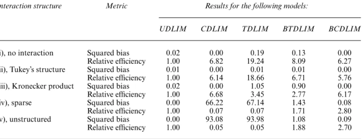
Results for the setting with main effects generated from a cubic DL function are summarized in Table 1. As we can observe in scenario (i), e.g. no interaction, all methods are more efficient than the UDLIM with relative efficiency ranging from 6.27 to 19.24. The empirical squared bias is minimal for the UDLIM (0.02), CDLIM (0.00) and BCDLIM (0.00) and is moderately small for the TDLIM (0.19) and the BTDLIM (0.13). Null interaction is a special case of Tukey’s model

Table 1. Empirical squared bias and empirical relative efficiency (measured with respect to the MSE of the

UDLIM estimate) of marginal lagged effects across five two-dimensional DL interaction models based on 1000 simulation data sets†

Interaction structure Metric Results for the following models:

UDLIM CDLIM TDLIM BTDLIM BCDLIM

(i), no interaction Squared bias 0.02 0.00 0.19 0.13 0.00 Relative efficiency 1.00 6.82 19.24 8.09 6.27 (ii), Tukey’s structure Squared bias 0.01 0.00 0.01 0.01 0.00 Relative efficiency 1.00 6.14 18.66 6.71 5.76 (iii), Kronecker product Squared bias 0.02 0.00 1.05 0.90 0.00 Relative efficiency 1.00 6.68 3.45 2.77 6.17 (iv), sparse Squared bias 0.00 66.22 67.14 1.43 0.08 Relative efficiency 1.00 0.07 0.07 1.71 2.80 (v), unstructured Squared bias 0.00 93.08 93.98 1.08 0.09 Relative efficiency 1.00 0.05 0.05 1.88 2.70 †The lagged effects of both exposures are generated from the same cubic DL function.

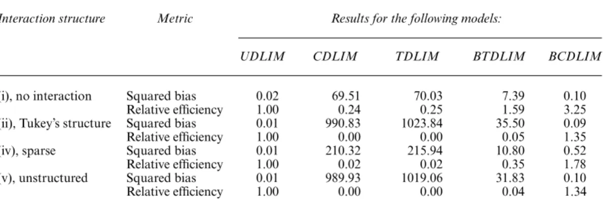
Table 2. Empirical squared bias and empirical relative efficiency (measured with respect to the MSE of the UDLIM estimate) of marginal lagged effects across five two-dimensional DL interaction models based on 1000 simulation data sets†

Interaction structure Metric Results for the following models:

UDLIM CDLIM TDLIM BTDLIM BCDLIM

(i), no interaction Squared bias 0.02 69.51 70.03 7.39 0.10 Relative efficiency 1.00 0.24 0.25 1.59 3.25 (ii), Tukey’s structure Squared bias 0.01 990.83 1023.84 35.50 0.09 Relative efficiency 1.00 0.00 0.00 0.05 1.35 (iv), sparse Squared bias 0.01 210.32 215.94 10.80 0.52 Relative efficiency 1.00 0.02 0.02 0.35 1.78 (v), unstructured Squared bias 0.01 989.93 1019.06 31.83 0.10 Relative efficiency 1.00 0.00 0.00 0.04 1.34 †The lagged effects of both exposures are generated from the same cubic-like DL function (moderate departure from a cubic function).

withη=0. Because TDLIMs correctly specify the main effects and interaction effects with a smaller number of parameters, it achieves the highest efficiency (19.24). In scenario (ii) where the non-null interaction effects are of Tukey form, all methods have similar, though slightly smaller, relative efficiency in comparison with scenario (i), ranging from 5.76 to 18.66. Again, the TDLIM has the highest relative efficiency as expected. Scenario (iii) represents the situation where the true interaction structure departs from Tukey’s form. We can see now that the TDLIM (3.45) is less efficient than the CDLIM (6.68) because of the bias that is introduced in estimating the interaction surface. However, the TDLIM is still more efficient than the UDLIM (1.00) and the BTDLIM (2.77). The CDLIM correctly specifies both main effects and interaction effects in this scenario and attains the highest efficiency.

Across scenarios (i) and (ii), we note that the squared bias and relative efficiency of the BTDLIM always fall between those of the CDLIM and TDLIM, suggesting that the BTDLIM successfully performs shrinkage and achieves a better average performance. In addition, we can observe that the BCDLIM (relative efficiency 6.27, 5.76, 6.17) is slightly less efficient than the CDLIM (relative efficiency 6.82, 6.14, 6.68) across the three scenarios. The difference is due to the flexibility of the BCDLIM that accounts for a possible departure from Kronecker product type of interaction structure. Scenarios (iv) and (v) are situations where the UDLIM is the only method that can unbiasedly estimate the interaction surface. As expected, both the CDLIM and the TDLIM suffer from serious bias and the gains of efficiency from dimension reduction diminish substantially. The class of interaction surfaces that the CDLIM and TDLIM can describe is restricted. Note that all the methods jointly estimate the main effects and interaction effects and thus misspecifying the interaction effects could possibly distort the estimation of the main effects as they are not orthogonal. The BCDLIM is less biased and more efficient than the BTDLIM across the two scenarios. Across all scenarios when the main effects are correctly specified, the BCDLIM has the best average performance in terms of estimation efficiency.

We summarize the results where the main effects deviate from a cubic DL function in Table 2. Both the CDLIM and the TDLIM are seriously biased, largely because of the misspecification of the main effect terms. These two methods are the least efficient. If we contrast scenarios (i) and (ii), we can observe that misspecification of the main effects not only influences the accuracy of estimation of the main effect DL function, but also the interaction DL surface. The BTDLIM

is biased across the board as well, with squared bias ranging from 7.39 to 35.50 respectively. It is more efficient than the UDLIM only in situations where there is no interaction. The BCDLIM is slightly biased across different scenarios with the squared bias ranging from 0.09 to 0.52. The BCDLIM leads to gains in efficiency with reduced bias. The relative efficiencies are 3.25, 1.35, 1.78 and 1.34 across the four scenarios. Summarizing the results in Tables 1 and 2, it is clear that the BCDLIM approach has desirable MSE properties across the scenarios, offering a robust and efficient solution to this problem.

4. Application

4.1. Data overview and modelling

We apply the five methods compared in Section 3 to the NMMAPS data. We jointly model daily time series of

(a) PM10and

(b) O3

in association with all-cause non-accidental mortality counts in Chicago, Illinois, for the period between 1987 and 2000. Details with respect to data assembly are available from http:// www.ihapss.jhsph.edu/data/NMMAPS/. Zanobettiet al.(2000) indicated that it is un-likely that lags beyond 2 weeks would have a substantial effect. We therefore setL1=L2=14 for PM10and O3levels respectively.

Previous studies showed that it is crucial to account for meteorologic variables as potential confounders in the analysis of air pollution effects (Welty and Zeger, 2005). Dominiciet al.(2005, 2007) highlighted the need to adjust carefully for a broad set of confounders and to explore their functional forms. We specify the adjustment covariates in the same way as Dominiciet al.(2005) and focus on the choice of the lag structure in our application. We acknowledge that there may be more optimal adjustment models when we introduce interaction effects. Letx1tk,x2tk,y_tk andz_tk denote the PM10level, O3level, mortality count and vector of time varying covariates,

measured on daytfor age groupkfort=1,: : :, 5114 andk=1, 2, 3 respectively. The three age categories are ‘greater than or equal to 75 years old’, ‘between 65 and 74 years old’ and ‘less than 65 years old’. PM10and O3were shared exposures across the three age groups so we have xltk≡xltforl=1, 2. For each groupk, we assume that, given PM10, O3and other time varying

confounders, the mortality count in Chicago on dayt is a Poisson random variableY_tk with meanμ_tk such that

log.μtk/=XT_1tβ₁+X_2tTβ₂+XT_Itγ+zT_tkα =XT 1tβ1+X2tTβ2+XTItγ+α0+ 2 j=1α1jI.k=j/+ 6 j=1α2jI.dowt=j/ +ns.temp_t; 6 DFs,α3/+ns.temp.3/_t ; 6 DFs,α4/ +ns.dptp_t; 3 DFs,α5/+ns.dptp.3/_t ; 3 DFs,α6/ +ns.t; 98 DFs,α7/+ns.t; 14 DFs,α8/I.k=1/+ns.t; 14 DFs,α9/I.k=2/ where X1t=.x1t,: : :,x1,t−14/T,X2t=.x2t,: : :,x2,t−14/T,XIt=X1t⊗X2t and ns.·/denotes the

natural spline with specified DFs. Predictors dow_t, temp_t, temp_t, dptp_tand dptp_trepresent the day of the week, the current day’s temperature, adjusted average lag 1–3 temperature, the current day’s dewpoint temperature and the adjusted average lag 1–3 dewpoint temperatures for dayt. The indicator variables allow different baseline mortality rates within each age group and within

each day of the week. The smooth term for timetis to adjust for long-term trends and seasonality and the choice of 98 DFs corresponds to 7 DFs per year over the 14-year time horizon. The last two product terms separate smooth functions of time with 2 DFs per year for each age group contrast. The primary goal is to estimate the coefficientsβ₁,β₂andγ, whereasαis the set of covariate parameters. A four-degree polynomial DL function is applied to bothβ₁andβ₂for the CDLIM, TDLIM, BTDLIM and BCDLIM. The analysis is performed in R version 3.3.1

and the source code is available from https://github.com/yinhsiuc/NMMAPS DLIM.

The computational times are provided in the on-line supplementary appendix A.4 Table 2 and the summary statistics corresponding to PM10 and O3 levels are provided in supplementary

appendix A.7.

4.2. Estimating marginal distributed lag function

The quantity 100 exp{10.β1_i+xÅ₂ΣL2

n=0γin/}represents the percentage change in daily mortality

that is associated with an increase of 10μg m−3 in PM10 level at lag iwhen the O3 level is

atxÅ₂ parts per billion. Similarly, the quantity 100 exp{10.β2j+xÅ₁ΣL1

m=0γmj/} represents the

percentage change in daily mortality that is associated with an increase in O3level of 10 parts

per billion at lagj when PM10 is set atxÅ1 μg m−3. We present the marginal lagged effects of

PM10 and O3 levels in Figs 1 and 2. If we look across the panels in Fig. 1, we can observe

that the fits of the UDLIM are undersmoothed and the fits of the CDLIM and TDLIM are oversmoothed, whereas those of the BTDLIM and BCDLIM are in between. When O3is at the

summer average level, the oversmoothing of the CDLIM and TDLIM results in underestimation of the PM10 effect at lag 3. For instance, the estimated percentage increases in mortality are

associated with an increase of 10μg m−3in PM10level at lag 3 when the O3level is at average

summer level are 0.53%, 0.14%, 0.03%, 0.23% and 0.36% for the UDLIM, CDLIM, TDLIM, BTDLIM and BCDLIM respectively. The lower bounds of 95% confidence or credible intervals for the methods except the TDLIM are appreciably above zero. In this situation, shrinkage methods are more desirable since the CDLIM and TDLIM misspecify the DL function and potentially underestimate the relative lag effects. Similarly, we observe slight oversmoothness of the CDLIM and TDLIM on the O3effect in Fig. 2. However, the degree of underestimation of

the O3effect at early lags is smaller. More similar DL functions across all methods except the

UDLIM indicate that the potential misspecification of the DL function by using the CDLIM and TDLIM is minimal.

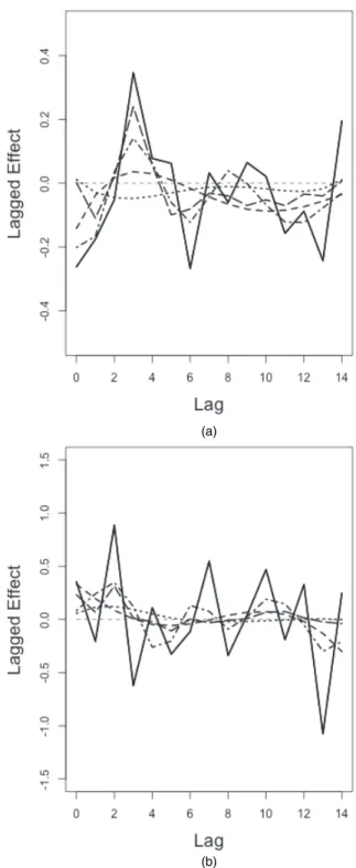
We present the marginal DL functions of PM10and O3levels by integrating out the other

pollutant in Fig. 3. Similarly to earlier findings, shrinkage is more needed for PM10 as the

CDLIM and TDLIM tend to oversmooth the DL function in this situation. In addition, we observe that the DL function for PM10 level starts from negative, grows to 0 and peaks at

lag 3, whereas the DL function for O3level is greater than 0 at lag 0 and peaks at lag 2. The

earlier peak for O3compared with PM10 suggests a more acute effect of O3than PM10with

an earlier window of susceptibility. We also observe that the UDLIM fits of O3fluctuate more

drastically than the UDLIM fits of PM10. This is explained by the stronger auto-correlation

of the O3time series and smoothing the DL function is certainly needed and preferred in this

case. We can observe that some of the estimated lagged effects are negative at larger lags for PM10. This phenomenon is denoted as mortality displacement (Zanobettiet al., 2000) and has

been discovered in previous studies. Mortality displacement, which is also referred to as the harvesting effect (Zanobettiet al., 2000), is the temporal shift of mortality. Usually a higher mortality rate due to the deaths of frail individuals a couple of days after a high air pollution episode is followed by a compensatory reduction in mortality rate due to the death of the more frail individuals.

( a )( b ) (d) (e) (c) Fig. 1. Estimated DL functions up to 14 da ys fo r the eff ects of PM 10 on mor tality in Chicago , Illinois , from 1987 to 2000 based on data from the NMMAPS under fiv e estimation methods (in all panels , O3 le v els are fix ed at the a v er age ser ies le v els in winter ( ) and the a v er age ser ies le v els in summer ( ); , estimated DL function relativ e to P M10 when O3 is disregarded in a single-pollutant model fo r P M10 ; lag eff ects are presented as the percentage change in mor tality that is associated with a 1 0 μ gm 3increase in PM 10 le v el): (a) UDLIM; (b) CDLIM; (c) TDLIM; (d) BTDLIM; (e) BCDLIM

( a )( b ) (d) (e) (c) Fig. 2. Estimated DL functions up to 14 da ys fo r the eff ects of O3 on mor tality in Chicago , Illinois , from 1987 to 2000 based on data from the NMMAPS under fiv e estimation methods (in all panels , P M10 le v els are fix ed at the a v er age ser ies le v els in winter ( ) and the a v er age ser ies le v els in summer ( ); , estimated DL function relativ e to O3 when PM 10 is disregarded in a single-pollutant model fo r O3 ;lag eff ects are presented as the percentage change in mor tality that is associated with a 1 0 par ts per billion increase in O3 le v el): (a) UDLIM; (b) CDLIM; (c) TDLIM; (d) BTDLIM; (e) BCDLIM

(a)

(b)

Fig. 3. Estimated DL functions up to 14 days for the effects of (a) PM10and (b) O3on mortality in Chicago,

Illinois, from 1987 to 2000 based on data from the NMMAPS under five estimation methods (the DL functions presented here are estimated by integrating out the other pollutant; lag effects are presented as the percentage change in mortality that is associated with a 10μg m3increase in PM10and a 10 parts per billion increase in O3): , UDLIM; , CDLIM; , TDLIM; - – - –, BTDLIM; — —, BCDLIM

4.3. Assessing interaction effects

Within each panel of Figs 1 and 2, we note that the estimated DL functions of one pollutant vary with the level of the other pollutant, indicating that PM10might moderate the effect of O3and

vice versa. For the UDLIM, CDLIM and TDLIM, we conducted a likelihood ratio test to test for PM10–O3-interactions and thep-values are 1:65×10−11 (225 DFs), 5:33×10−9(25 DFs)

and less than 10−4(1 DF) respectively. The precision of thep-value of the TDLIM is only up to 10−4because of finite bootstrap samples. For the two shrinkage methods the BTDLIM and BCDLIM, we computed the difference in deviance information criterion (DIC) (Spiegelhalter

et al., 2002) between the models with and without interaction. The DIC differences are 25.56 and 68.35 respectively. It is difficult to determine a clear threshold of DIC difference for model selection (Plummer, 2008). However, models with smaller DIC are generally preferred when DIC differences are greater than 10. Coupled with thep-values that are obtained from the frequentist approaches, we conclude that the interaction between PM10and O3is evident.

From Figs 1 and 2, we can see that the summer curves are above the winter curves, suggesting that PM10and O3have synergistic effects on each other. Furthermore, we observe that the gaps

between the curves of the three quartiles decrease beyond lag 6 and that happens across the board. The interaction between PM10and O3occurs at early lags. We added a dotted curve in each panel

for the estimated DL function from a single-pollutant analysis (i.e. models with PM10alone or

O3alone), representing the ‘average’ DL effects if we disregard the interaction effect between

the two pollutants. The evidence in favour of looking at PM10and O3jointly is compelling. 5. Discussion

In analysing NMMAPS data, we demonstrated the importance of accounting for interaction between the PM10and O3 time series when modelling the joint pollution effect on mortality.

Two major pieces of evidence support the existence of pollutant–pollutant interaction— (a) the marginal DL function of one pollutant varies when the level of the other changes, and (b) the smallp-values from frequentist approaches and the large DIC values from the Bayesian

approaches suggest evidence in favour of a PM10×O3interaction.

This adds to the finding of previous studies that supported the idea of a plausible synergism involving PM10and O3(Mauderly and Samet, 2009).

In this paper, we presented five strategies to model lagged effects of two pollutants in a joint model. We reviewed two existing frequentist methods the UDLIM and CDLIM, and we proposed a frequentist TDLIM using Tukey’s interaction structure, its Bayesian version and a Bayesian approach to perform shrinkage between the UDLIM and CDLIM. There are two major novelties. We adopted Tukey’s 1 DF interaction structure to model two-way interactions parsimoniously. The estimation is efficient and the interaction testing is powerful. We also introduced the Bayesian version of the TDLIM (i.e. the BTDLIM) and the Bayesian version of the CDLIM (i.e. the BCDLIM). These Bayesian models allow for a departure from a prespecified structure of a DL function or surface and have been shown to be robust to misspecification. They are data adaptive and can achieve bias–variance trade-off.

Each of the five approaches has some limitations that we discuss below. The UDLIM is unbi-ased but potentially less efficient, especially when the auto-correlation between serial pollution measurement is large. The CDLIM imposes some structure to constrain the lag coefficients and can potentially achieve greater estimation precision. In practice, we recommend a DL structure that is no more complex than a cubic polynomial as the default choice since it is usually suffi-cient to capture the observed non-linear patterns as a function of the lags. Nonetheless, when the

DL structure is misspecified, the model-dependent CDLIM estimator can be seriously biased. Tukey’s type of interaction has mostly been used for hypothesis testing rather than estimation in previous research. Expressing interaction effects as a scaled product of the corresponding main effects implies that the interaction effects can be non-zero only when the main effects are non-zero. This hierarchical feature results in a lack of identifiability for the scaled parameter in Tukey’s model when the main effects are not present. In addition, Tukey’s model is not invariant to location shifts. Different centring schemes lead to different estimates of the scale parameter

ηand no universal remedy exists.

The hierarchical BCDLIM is robust to misspecification of the DL structure. The data-adaptive shrinkage can be regarded as an automatic procedure to attain a balance between the more gen-eral UDLIM and the more constrained CDLIM. The full rank transformation on the UDLIM imposes smoothness on the shrinkage path and anya prioriknowledge about the DL structure can be incorporated. It is important to note that the BCDLIM can be extended to explore higher order interaction and multiple-pollutant scenarios. We also tried to adapt the HDDLM to two-pollutant scenarios. However, the unmodified predictive process interpolator (Banerjee

et al., 2008), which is the major technique that is used in HDDLMs for dimension reduction (Finleyet al., 2009), leads to overly smooth DL functions or surfaces which result in seriously biased estimates. We therefore decided not to include the HDDLM in this paper.

The two-pollutant DLIMs can be directly combined with DL non-linear models (Gasparrini

et al., 2010) to capture non-linear exposure–outcome associations flexibly by replacing the linear terms in DLM specifications with some basis functions (e.g.B-splines). As indicated by Heet al.

(2015), failing to account for non-linear main effects may lead to spurious detection of linear interaction terms. However, when the covariates are correlated as in our application, the signals from non-linear main effects and linear interaction effects may be indistinguishable. In addition, some regularization may be needed in this high dimensional situation to avoid overfitting. We consider this line of extension for future research.

The two-pollutant DLIM approaches that are introduced in this paper can also be extended to multipollutant situations where up to two-way interactions are considered. If one would like to consider higher order interactions and/or non-linear interactions, extension of tree-based approaches such as classification and regression trees and the Bayesian kernel machine regression can be promising. In some situations, choosing the most important pollutants among multiple candidates that are associated with a health outcome is the primary goal.

In real world settings, it is usually difficult to validate the underlying assumptions of a model-based estimator. The notion of data-adaptive shrinkage is attractive when no single estimator is universally optimal. When facing uncertainty, robust models such as the BCDLIM that have better average performance are more desirable. The BCDLIM can potentially be extended to areas outside environmental epidemiology. We hope that our work will lead to more attempts in developing two-dimensional and multi-dimensional DLIMs in the future.

Acknowledgements

The research is supported by National Science Foundation grant DMS 1406712 and National Institutes of Health grant ES 20811.

References

Almon, S. (1965) The distributed lag between capital appropriations and expenditures.Econometrica,33, 178–196. Banerjee, S., Gelfand, A. E., Finley, A. O. and Sang, H. (2008) Gaussian predictive process models for large

Billionnet, C., Sherrill, D. and Annesi-Maesano, I. (2012) Estimating the health effects of exposure to multi-pollutant mixture.Ann. Epidem.,22, 126–141.

Bobb, J. F., Valeri, L., Henn, B. C., Christiani, D. C., Wright, R. O., Mazumdar, M., Godleski, J. J. and Coull, B. A. (2014) Bayesian kernel machine regression for estimating the health effects of multi-pollutant mixtures. Biostatistics,16, 493–508.

Chatterjee, N., Kalaylioglu, Z., Moslehi, R., Peters, U. and Wacholder, S. (2006) Powerful multilocus tests of genetic association in the presence of gene-gene and gene-environment interactions.Am. J. Hum. Genet.,79, 1002–1016.

Dominici, F., McDermott, A., Daniels, M., Zeger, S. L. and Samet, J. M. (2005) Revised analyses of the National Morbidity, Mortality, and Air Pollution Study: mortality among residents of 90 cities.J. Toxicol. Environ. Hlth A,68, 1071–1092.

Dominici, F., Peng, R. D., Barr, C. D. and Bell, M. L. (2010) Protecting human health from air pollution: shifting from a single-pollutant to a multi-pollutant approach.Epidemiology,21, 187–194.

Dominici, F., Peng, R. D., Bell, M. L., Pham, L., McDermott, A., Zeger, S. L. and Samet, J. M. (2006) Fine particulate air pollution and hospital admission for cardiovascular and respiratory diseases.J. Am. Med. Ass.,

295, 1127–1134.

Dominici, F., Peng, R. D., Ebisu, K., Zeger, S. L., Samet, J. M. and Bell, M. L. (2007) Does the effect of PM10 on mortality depend on PM nickel and vanadium content?: A reanalysis of the NMMAPS data.Environ. Hlth Perspect.,115, 1701–1703.

Finley, A. O., Sang, H., Banerjee, S. and Gelfand, A. E. (2009) Improving the performance of predictive process modeling for large datasets.Computnl Statist. Data Anal.,53, 2873–2884.

Gasparrini, A., Armstrong, B., and Kenward, M. G. (2010) Distributed lag non-linear models.Statist. Med.,29, 2224–2234.

Gelman, A. (2006) Prior distributions for variance parameters in hierarchical models (comment on article by Browne and Draper).Baysn Anal.,1, 515–534.

He, Z., Zhang, M., Lee, S., Smith, J. A., Guo, X., Palmas, W., Kardia, S. L., Roux, A. V. D. and Mukherjee, B. (2015) Set-based tests for genetic association in longitudinal studies.Biometrics,71, 606–615.

Heaton, M. J. and Peng, R. D. (2014) Extending distributed lag models to higher degrees.Biostatistics,15, 398– 412.

Hu, W., Mengersen, K., McMichael, A. and Tong, S. (2008) Temperature, air pollution and total mortality during summers in Sydney, 1994–2004.Int. J. Biometeorol.,52, 689–696.

Lunn, D., Spiegelhalter, D., Thomas, A. and Best, N. (2009) The BUGS project: evolution, critique and future directions.Statist. Med.,28, 3049–3067.

Maity, A., Carroll, R. J., Mammen, E. and Chatterjee, N. (2009) Testing in semiparametric models with interaction, with applications to gene–environment interactions.J. R. Statist. Soc.B,71, 75–96.

Marx, B. D. and Eilers, P. H. (1998) Direct generalized additive modeling with penalized likelihood.Computnl Statist. Data Anal.,28, 193–209.

Mauderly, J. L. (1993) Toxicological approaches to complex mixtures.Environ. Hlth Perspect.,101, 155–165. Mauderly, J. L. and Samet, J. M. (2009) Is there evidence for synergy among air pollutants in causing health

effects?Environ. Hlth Perspect.,117, 1–6.

Muggeo, V. M. (2007) Bivariate distributed lag models for the analysis of temperature-by-pollutant interaction effect on mortality.Environmetrics,18, 231–243.

Plummer, M. (2008) Penalized loss functions for Bayesian model comparison.Biostatistics,9, 523–539. Pope, C. A. and Dockery, D. W. (2006) Health effects of fine particulate air pollution: lines that connect.J. Air

Waste Mangmnt Ass.,56, 709–742.

Pope, C. A., Dockery, D. W. and Schwartz, J. (1995) Review of epidemiological evidence of health effects of particulate air pollution.Inhaln Toxicol.,7, 1–18.

R Core Team (2017)R: a Language and Environment for Statistical Computing. Vienna: R Foundation for Statistical Computing.

Roberts, S. (2005) An investigation of distributed lag models in the context of air pollution and mortality time series analysis.J. Air Waste Mangmnt Ass.,55, 273–282.

Spiegelhalter, D. J., Best, N. G., Carlin, B. P. and van der Linde, A. (2002) Bayesian measures of model complexity and fit (with discussion).J. R. Statist. Soc.B,64, 583–639.

Sun, Z., Tao, Y., Li, S., Ferguson, K. K., Meeker, J. D., Park, S. K., Batterman, S. A. and Mukherjee, B. (2013) Statistical strategies for constructing health risk models with multiple pollutants and their interactions: possible choices and comparisons.Environ. Hlth,12, 85–103.

Tibshirani, R. (1996) Regression shrinkage and selection via the lasso.J. R. Statist. Soc.B,58, 267–288. Tukey, J. W. (1949) One degree of freedom for non-additivity.Biometrics,5, 232–242.

Welty, L. J., Peng, R., Zeger, S. and Dominici, F. (2009) Bayesian distributed lag models: estimating effects of particulate matter air pollution on daily mortality.Biometrics,65, 282–291.

Welty, L. J. and Zeger, S. L. (2005) Are the acute effects of particulate matter on mortality in the National Morbidity, Mortality, and Air Pollution Study the result of inadequate control for weather and season?: A sensitivity analysis using flexible distributed lag models.Am. J. Epidem.,162, 80–88.

M., Goren, A., Forsberg, B., Michelozzi, P., Rabczenko, D., Aranguez Ruiz, E. and Katsouyanni, K. (2002) The temporal pattern of mortality responses to air pollution: a multicity assessment of mortality displacement. Epidemiology,13, 87–93.

Zanobetti, A., Wand, M., Schwartz, J. and Ryan, L. (2000) Generalized additive distributed lag models: quantifying mortality displacement.Biostatistics,1, 279–292.

Supporting information

Additional ‘supporting information’ may be found in the on-line version of this article: ‘Supplementary appendix for “Distributed lag interaction models with two pollutants”’.