HAL Id: hal-01811322
https://hal.archives-ouvertes.fr/hal-01811322
Submitted on 24 Jan 2020
HAL
is a multi-disciplinary open access
archive for the deposit and dissemination of
sci-entific research documents, whether they are
pub-lished or not. The documents may come from
teaching and research institutions in France or
abroad, or from public or private research centers.
L’archive ouverte pluridisciplinaire
HAL, est
destinée au dépôt et à la diffusion de documents
scientifiques de niveau recherche, publiés ou non,
émanant des établissements d’enseignement et de
recherche français ou étrangers, des laboratoires
publics ou privés.
Global solution of non-convex quadratically constrained
quadratic programs
Sourour Elloumi, Amélie Lambert
To cite this version:
Sourour Elloumi, Amélie Lambert. Global solution of non-convex quadratically constrained quadratic
programs.
Optimization Methods and Software, Taylor & Francis, 2019, 34 (1), pp.98-114.
�10.1080/10556788.2017.1350675�. �hal-01811322�
constrained quadratic programs
Sourour Elloumi1 and Am´elie Lambert21 CEDRIC-ENSTA, 828 Boulevard des Mar´echaux, 91120 Palaiseau, France
{sourour.elloumi}@ensta-paristech.fr
2 CEDRIC-CNAM, 292 rue saint Martin, F-75141 Paris Cedex 03, France
Abstract. The class of mixed-integer quadratically constrained quadratic programs (QCQP) consists of minimizing a quadratic function under quadratic constraints where the variables could be integer or continuous. On a previous paper we introduced a method calledMIQCRfor solving QC-QPs with the following restriction : all quadratic sub-functions of purely continuous variables are already convex. In this paper, we propose an extension of MIQCR which applies to any QCQP. Let (P) be a QCQP. Our approach to solve (P) is first to build an equivalent mixed-integer quadratic problem (P∗). This equivalent problem (P∗) has a quadratic convex objective function, linear constraints, and additional variablesy
that are meant to satisfy the additional quadratic constraintsy=xxT, where x are the initial variables of problem (P). We then propose to solve (P∗) by a branch-and-bound algorithm based on the relaxation of the additional quadratic constraints and of the integrality constraints. This type of branching is known as spatial branch-and-bound. Compu-tational experiences are carried out on a total of 325 instances. The results show that the solution time of most of the considered instances is improved by our method in comparison with the recent implementation of QuadProgBB, and with the solvers Cplex,Couenne,Scip,BARON and
GloMIQO.
Key words: General mixed-integer quadratic programming, Global optimiza-tion, Spatial branch-and-bound, Quadratic convex relaxaoptimiza-tion, Experiments
1
Introduction
We consider the problem of optimizing a quadratic function subject to quadratic and bound constraints:
(P) minf0(x)≡ hQ0, xxTi+cT0x s.t. fr(x)≡ hQr, xxTi+cTrx≤br r= 1, . . . , m `≤x≤u xi∈N ∀i∈J xi∈R ∀i∈I\J with hA, Bi = n X i=1 n X j=1 aijbij, and where I = {1, . . . , n}, J ⊂ I, ∀r = 0, . . . , m
(Qr, cr)∈ Sn×Rn, b∈Rm, andu∈Rn. Without loss of generality we suppose
that l∈Rn
+. We denote bySn the set ofn×nsymmetric matrices, by Sn+ the
set of positive semidefinite matrices of Sn andM 0 means thatM ∈ Sn+. We
also denote by 0n the zero n×n matrix and byI2 the cartesian product of a
setI by itself.
We assume the feasible domain of (P) to be non-empty. Problem (P) trivially contains the case where there are quadratic equalities, since an equality can be replaced by two inequalities. It also contains the case of linear constraints since a linear equality is a quadratic constraint with a zero quadratic part.
Problem (P) is a Mixed-Integer Quadratically Constrained Program (MIQCP) and belongs to the class of N P-hard problems [37]. It arises in many applica-tion areas such as graph theory [38], market prices computaapplica-tion [44], or the pooling problem introduced by Haverly [7, 40]. Several applications of the box-constrained case, namely, when J =∅ and the only constraints are `≤x≤u were mentioned by Mor´e and Toraldo in [49]. Moreover, (P) generalizes sev-eral difficult problems such as binary programming, fractional programming, or polynomial programming. This is due to the fact that these problems can be re-formulated Redinto a MIQCP. Binary quadratic programming has itself a large set of applications. We refer the reader to recent surveys on more general mixed integer non linearproblems [25].
Exact solution methods for solving (P) generally use the well-known branch-and-bound algorithm. Key operations of this algorithm are called bounding and branching. Bounding often relies on the computation of a lower bound (for a minimization problem) by solving a relaxed problem of the initial one. There are several bounding strategies. Among others, three strategies are classically used: approximation of the convex envelope of each quadratic term [45], outer approximation of convex terms [21, 30, 31], or computation of a bound thanks to semidefinite relaxations [6, 52]. Branching strategies depend on the nature of the variables. For integer variables, branching is commonly done by recursively dividing the solution set into two subsets in such a way that a current fractional solution is discarded. This represents a hope to improve the bounds further ob-tained by the relaxation in the two subsets. For continuous variables, branching is done by considering a variable xi whose current interval is [`i, ui], choosing
some value ¯xi in ]`i, ui[, and dividing the solution set into two subsets, one with
interval [`i,x¯i] and the other with interval [¯xi, ui] for variable xi. Doing this
does not directly discard undesired points but may change the structure of the relaxed problem. This branching is called spatial branch-and-bound (sBB) in the global optimization literature and is due to Falk and Soland [32]. Finally, a sBB algorithm can be improved by computing feasible local solutions.
Several versions of the sBB algorithm were proposed [9, 55, 56, 54, 61, 62]. Three classical relaxations can be used to perform a sBB. The first and most common version uses a linear relaxation of (P) tightened by cuts such as the reformulation-linearization technique (RLT) [53]. Some softwares, implement-ing the methods described above, are available for solvimplement-ing (P). See for in-stance Couenne 0.5 [11], Baron [51], Scip 3.2.1 [1, 58]. Another frequently used technique to obtain convex relaxations of (P) is semi-definite program-ming, see for example [5, 52]. The last way is based on a non-linear convex relax-ation and is called αBB [2–4, 24, 33–35, 59, 60]. It is implemented into software
GloMIQO 2[46–48]
Cplex 12.6.2 [20, 22, 42] and the recent solver QuadProgBB [27] also han-dle (P), but are limited to the case where all constraints are linear. The solver
QuadprogBBuses a finite branch-and-bound scheme, in which branching is based on the first-order KKT conditions. Moreover, polyhedral-semidefinite relaxations are solved at each node of the branch-and-bound tree. In particular, their relax-ations are derived from completely positive and doubly nonnegative programs. In the last version of Cplex 12.6.2, a sBB algorithm is performed based on two different quadratic and convex relaxations of (P) built as follows: in the first one, (P) is reformulated as a separable problem where the diagonal Hessian matrix is chosen positive semi-definite, in the second one, a convex reformulation is built based on the factorized eigenvector space. Moreover,Cplex 12.6.2exploits the performances of Cplex for binary quadratic programs to solve box-constrained problems [22].
In this paper, we present a new sBB algorithm for solving (P) to -global optimality. In previous papers [15–17], we introduced quadratic convex refor-mulation methods to solve (P) with the following restriction : all quadratic sub-functions of purely continuous variables are already convex. More precisely, letf(a, b) be a quadratic function of integer variablesa, and of continuous vari-ables b. Function f(a, b) is a sum of monomials, and can be viewed as the sum of 2 functions: f1(a, b) that is composed of the mixed-integer monomials, and f2(b) that corresponds to the monomials with only continuous variables. We call f2(b) the sub-function of purely continuous variables. Our contribution in this
paper is to handle the general quadratic case without any restriction over the pure-continuous sub-functions. One originality of our approach is that it is based on an equivalent quadratic reformulation of (P) which is computed thanks to semi-definite programming, in a pre-processing step. Then, a quadratic convex relaxation of the equivalent formulation is used as a bounding strategy within a sBB. To evaluate our algorithm, we present computational experiences on 325 instances coming from benchmarks of the literature. We compare our
al-gorithm with the recent implementation of QuadProgBB, and with the solvers
Cplex 12.6.2 [42], Couenne 0.5 [11], Scip 3.2.1 [58], BARON 17.3.31 and
GloMIQO 2[48]. We show on performance profiles that for these instances, our method outperforms the others for many large and high density instances.
The outline of the paper is the following. In Section 2, we review quadratic convex reformulation methods and situate the current paper compared to our previous ones. In Section 3, we present our new quadratic reformulation of (P) and we show that this reformulation is an improvement of the complete lin-earization standardly used within a sBB. Then, in Section 4, we describe the main features of our sBB based on the relaxation of the quadratic constraints yij =xixj and of the integrality constraints. In Section 5, we present our
com-putational results. Section 6 draws a conclusion.
2
Review of Quadratic Convex Reformulations
Problem (P) presents two difficulties: non-convexity of functions fr and the
integrality of some of its variables. It is qualified as convex when all functions f0, . . . , fmare convex [50]. When (P) is convex and there are no integer variables
(J = ∅), we have a convex problem that can be solved in polynomial time. Thanks to the later property, convex problems with integer variables can be solved by a branch-and-bound based on continuous relaxation, as frequently done in quadratic convex solvers. Without these convexity assumptions, problem (P), even with only continuous variables, is significantly harder to solve.
In this paper, we present an algorithm based on a reformulation. By this, we mean an algorithm that works in two phases. In the first phase, an equivalent for-mulation to the initial problem is designed. The key idea is that one relaxation of the equivalent formulation is a convex problem. Finally, the equivalent formula-tion can be solved to-global optimality by a spatial branch-and-bound process based on this convex relaxation. This is the second phase of the algorithm.
In the presence of integer variables, many reformulation methods rely on the reformulation of a quadratic program into a MILP. This is called linearization. A very well-known linearization for quadratic programs with binary variables is due to Fortet [36] and consists in replacing any product of two binary variables xiandxj by an additional variableyij, together with a set of linear constraints
enforcing the equality yij =xixj. The idea of linearization can be extended to
quadratic programs with general bounded integer variables with a tricky binary expansion of the general integers [14]. The obtained MILP is then solved by branch-and-bound or branch-and-cut. Linearization is also used for continuous variables. An equivalent problem is built where the only non-linearity is in the equalityyij =xixj. This equality is then relaxed in each node and enforced by
a spatial branch-and-bound.
Another alternative to linearization consists in reformulating a non-convex quadratic program with binary variables into a convex quadratic program with the same variables. This idea appeared in Hammer and Rubin [39] where the
authors use the equality x2
i = xi which holds for any binary variable xi, and
the smallest (resp. largest) eigenvalue in order to shift the diagonal terms of the Hessian matrix of the objective function and obtain an equivalent convex (resp. concave) function. Another simple quadratic convex reformulation was proposed in [12]. This reformulation, also based onx2
i =xi, transforms every non-convex
productxixj into the convex function 12((xi+xj)2−xi−xj) or to the concave
function 12(−(xi−xj)2+xi+xj). These simple quadratic convex reformulations,
while being very easy to implement, often lead to inefficient methods because their continuous relaxation bound may be very poor.
Considering the problem of minimizing a quadratic function of binary vari-ables, Billionnet and Elloumi [13] introduced the question of how to change the diagonal terms of the Hessian matrix in such a way that (i) the obtained function is convex, and (ii) the continuous relaxation bound of this function is as tight as possible. The authors prove that, in this regard, “optimal” diagonal terms can be obtained from the dual solution of a semidefinite programming relaxation of the initial problem. With these optimal diagonal terms, the continuous relax-ation bound is equal to the semidefinite programming relaxrelax-ation bound. The reformulation idea and the solution method were then extended in [19] to the case of binary quadratic programs with linear equalities and the acronym QCR
for Quadratic Convex Reformulation was born. Here, the SDP relaxation whose solution gives the best reformulation contains the so-called RLT constraints, obtained by multiplying the linear inequalities by the variables in order to get stronger relaxations.
Further extentions were designed in Billionnet et al. [15] for the case of bounded integer variables but still with linear constraints. In this case, a bi-nary expansion of the initial variables is performed, together with the addition of new variablesyijthat represent the product of two general integer variablesxi
andxj. These additional variables allow to widen the family of potential
refor-mulations since any perturbation of each element of the Hessian matrix is now considered. In this extension, a quadratic program with linear constraints and bounded integer variables is considered. The reformulation phase is based on a stronger SDP relaxation, sometimes called “Shor+RLT” in the literature [6]. The reformulated problem is a convex quadratic problem with continuous and binary variables, which is again solved by a quadratic convex programming solver. We present an extension to the case where the initial quadratic problem contains continuous variables in Billionnet et al. [15]. But, we had the following restric-tion: in the objective function, all quadratic sub-functions of purely continuous variables are already convex. This extension was called MIQCR (Mixed Integer Quadratic Convex Reformulation).
Another extension is obtained in [17] to the case of programs with quadratic inequalities, with the same kind of restriction on the quadratic sub-functions of purely continuous variables. The quadratic convex reformulation is presented in a new setting which includes linearization as a particular case. More precisely, the equivalent problem has additional variables yij, additional quadratic
These quadratic constraints are linearized by the addition of a large number of variables (binary expansion) and constraints. The obtained equivalent problem is a mixed-integer quadratic program with a convex objective function and linear constraints. It can be solved by a mixed-integer quadratic convex solver. How-ever, in the presence of convex purely continuous sub-functions, the “Shor+RLT” relaxation cannot yet be used for computing the reformulation, hence, in this case we use a weaker SDP relaxation than in the current paper.
For the linearly constrained case, we introduced in [16], a specific branch-and-bound algorithm to solve the equivalent formulation. Constraintsyij =xixj are
not linearized but are rather enforced within a branch-and-bound process based on the relaxation of these quadratic constraints only, i.e. we keep the integrality constraints.
In this paper, contrarily to the reformulation proposed in [15, 17], and fol-lowing the ideas of [16], we keep in our reformulation the non-convex quadratic constraintsyij =xixj. To solve the reformulated problem, we design a sBB based
on the relaxation of constraintsyij =xixj and of the integrality constraints. In
contrast to [17], not only we obtain convex relaxations of smaller size, but we can also handle general quadratic problems.
3
A quadratic reformulation of (P
)
We consider any set of positive semi-definite matrices S0, . . . , Sm. We also lift
the problem to a higher space by introducing variables yij that are meant to
satisfy yij = xixj. We build the following equivalent quadratic formulation to
(P): (PS0,...,Sm) min f0,S0(x, Y)≡ hS0, xxTi+cT0x+hQ0−S0, Yi s.t. fr,Sr(x, Y)≡ hSr, xxTi+cTrx+hQr−Sr, Yi ≤br r= 1, . . . , m(1) yij≤ujxi+lixj−ujli (i, j)∈I2, i≤j (2) yij≤uixj+ljxi−uilj (i, j)∈I2, i≤j (3) yij≥ujxi+uixj−uiuj (i, j)∈I2, i≤j (4) yij≥ljxi+lixj−lilj (i, j)∈I2, i≤j (5) yii≥xi i∈J (6) yij=yji (i, j)∈I2, i < j (7) yij=xixj (i, j)∈I2 (8) xi∈N ∀i∈J (9) To build (PS0,...,Sm), we introduce n
2 new variables Y to model the
prod-uctsxixj (Constraints (8)). Then, we formulate fr(x) as a sum of a quadratic
function of thexvariables and a linear function of theY variables. It holds that fr,Sr(x, Y) is equal tofr(x) ifyij =xixj. We also add the well-known McCormick
inequalities (2) - (5) [45], and Constraints (6) that come from x2
i ≥xi, a valid
inequality for general integer variables to tighten the relaxation. Because ma-tricesS0, . . . Sm are positive semidefinite, the reformulated problem (PS0,...,Sm)
has the property that when Constraints (8) and (9) are relaxed, it is a convex problem. We call this convex relaxation (PS0,...,Sm).
We then consider the problem of finding the best set of positive semi-definite matricesS0, . . . , Sm, in the sense that the optimal solution value of (PS0,...,Sm)
is as large as possible. This amounts to solving the following problem (OP TS):
(OP TS)
max
S0,...,Sm0
v(PS0,...,Sm)
wherev(P) is the optimal value of problem (P). The following theorem shows thatv(OP TS) is equal to the optimal value of an SDP program which is a
semi-definite relaxation of (P).
Theorem 1. Let (SDP)be the following semi-definite program:
(SDP) minf(X, x) =hQ0, Xi+cT0x s.t. hQr, Xi+cTrx≤br r={1, . . . , m} (10) Xij−ujxi−lixj+ujli≤0 (i, j)∈I2, i≤j (11) Xij−uixj−ljxi+uilj ≤0 (i, j)∈I2, i≤j (12) −Xij+ujxi+uixj−uiuj ≤0 (i, j)∈I2, i≤j (13) −Xij+ljxi+lixj−lilj≤0 (i, j)∈I2, i≤j (14) −Xii+xi≤0 i∈J (15) 1 x xT X 0 (16) x∈Rn X ∈ S n (17)
It holds that v(OP TS) = v(SDP). Besides, the following positive
semi-definite matrices allow to build an optimal solution(S0∗, . . . , Sm∗)of(OP TS):
i) ∀r= 1, . . . , m,Sr∗=0n
ii) S0∗=Q0+
m
X
r=1
α∗rQr+Φ∗, where α∗ is the vector of optimal dual variables
associated with Constraints (10). MatrixΦ∗ is computed as:
Φ∗ii=Φ1ii∗+Φ2ii∗−Φ3ii∗−Φ4ii∗−ϕ∗i, Φ∗ij=Φ1ij∗+Φij2∗−Φ3ij∗−Φ4ij∗,
whereΦ1∗,Φ2∗,Φ3∗,Φ4∗ are the symmetric matrices built from the optimal dual variables associated with Constraints (11)–(14), and ϕ∗ is the vector of dual variables associated with Constraints (15).
Proof. This proof is similar to Proof of Theorem 1 in [17], but we now consider the case where the lower bounds`iover the variablesxcan be any non negative
reals, while in [17], `i was considered as 0. To prove Theorem 1, we show that
v(OP TS) =v(SDP) by showing thatv(OP TS)≤v(SDP) and thenv(OP TS)≥
v(SDP).
To prove that v(OP TS) ≤ v(SDP), we show that v(PS¯0,...,S¯m) ≤ v(SDP)
for any ¯S0, . . . ,S¯m∈ Sn+, which in turn implies thatv(OP TS)≤v(SDP) since
the right hand side is constant. For this, we show that if (¯x,X¯) is feasible for (SDP), then (x, Y) := (¯x,X¯) is i) feasible for (PS¯0,...,S¯m) and ii) its objective
value is less or equal thanv(SDP). Since (PS¯0,...,S¯m) is a minimization problem,
v(PS¯
0,...,S¯m)≤v(SDP) follows.
i) We prove that (x, Y) is feasible to (PS¯0,...,S¯m). Constraints(2)-(7) are
ob-viously satisfied from Constraints (11)–(15) and (17). We now prove that Constraints (1) are satisfied:
hS¯r, xxTi+cTrx+hQr−S¯r, Yi=hS¯r,x¯x¯Ti+cTrx¯+hQr−S¯r,X¯i
=hS¯r,x¯x¯T −X¯i+cTrx¯+hQr,X¯i
≤br from Constraints (10), since
¯
Sr0, and Constraint (16).
ii) Let us compare the objective values. For this, we prove that hS¯0,x¯x¯Ti+
cT
0¯x+hQ0−S¯0,X¯i − hQ0,X¯i −cT0x¯ ≤0 or that hS¯0,x¯x¯T −X¯i ≤0. This
last inequality follows from ¯S00 and Constraint (16).
Let us secondly prove that v(OP TS)≥v(SDP) or equivalently v(OP TS)≥
v(DSDP) where (DSDP) is the dual of (SDP). The following problem (DSDP) is the dual of (SDP): (DSDP) maxg(α, Φ) =− m X r=1 αrbr+hΦ1+Φ2, ulTi − hΦ3, uuTi − hΦ4, llTi s.t. Q0+ m X r=1 αrQr+Φ0 (18) c0+ m X r=1 αrcr−(Φ1+Φ2−2Φ3)Tu−(Φ1+Φ2−2Φ4)Tl+ϕ≥0 (19) Φ=Φ1+Φ2−Φ3−Φ4−diag(ϕ) (20) α∈Rm+, Φ∈ Sn, Φ1, Φ2, Φ3, Φ4 ∈ Sn, Φrij≥0∀(r, i, j), ϕ∈R n +
where α ∈ Rm+ are the dual variables associated to constraints (10), and Φi,
i= 1, . . . ,4 are the positive semidefinite matrices built from the dual variables θ associated with constraints (11), (12), (13), (14), respectively. For instance, if θ1is the dual variable associated to constraint (11), thenΦ1=θ1+θ1T
2 .ϕare the
we have Φ=Φ1+Φ2−Φ3−Φ4−diag(ϕ).
Let ( ¯α,Φ¯1,Φ¯2,Φ¯3,Φ¯4,ϕ¯) be a feasible solution to (DSDP) and let ¯Φ= ¯Φ1+
¯
Φ2−Φ¯3−Φ¯4−diag( ¯ϕ), then we build the following positive semidefinite matrices:
¯ Sr=0n r= 1, . . . , m ¯ S0=Q0+ m X r=1 ¯ αrQr+ ¯Φ
by Constraint (18), ( ¯S0, . . . ,S¯m) form a feasible solution to (OP TS). The
objec-tive value of this solution is equal tov(PS¯0,...,S¯m).
We now prove that v(PS¯0,...,S¯m) ≥ v(DSDP). For this, we prove that for
any feasible solution (¯x,Y¯) to (PS¯
0,...,S¯m), the associated objective value is not
smaller than g( ¯α,Φ¯). Denote by ∆the difference between the objective values, i.e.,∆=hS¯0,x¯x¯Ti+cT0x¯+hQ0−S¯0,Y¯i −g( ¯α,Φ¯). We below prove that∆≥0.
∆=hS¯0,x¯x¯Ti+c0Tx¯+hQ0−S¯0,Y¯i+ m X r=1 ¯ αrbr− hΦ1+Φ2, ulTi+hΦ3, uuTi+hΦ4, llTi ≥cT0x¯− h m X r=1 ¯ αrQr+ ¯Φ,Y¯i+ m X r=1 ¯ αrbr− hΦ1+Φ2, ulTi+hΦ3, uuTi+hΦ4, llTi since ¯S00, andQ0−S¯0=−( m X r=1 ¯ αrQr+ ¯Φ) =cT0x¯+ m X r=1 ¯ αr(br− hQr,Y¯i)− hΦ,¯ Y¯i − hΦ1+Φ2, ulTi+hΦ3, uuTi+hΦ4, llTi ≥cT0x¯+ m X r=1 ¯ αrcTrx¯− hΦ,¯ Y¯i − hΦ 1+Φ2, ulTi+hΦ3, uuTi+hΦ4, llTi
ascTrx¯+hQr,Y¯i ≤br and ¯αr≥0. Moreover, by Constraint (20) we get:
∆≥cT0x¯+ m X r=1 ¯ αrcTrx¯− hΦ¯ 1+ ¯Φ2 −Φ¯3−Φ¯4−diag( ¯ϕ),Y¯i − hΦ1+Φ2, ulTi+hΦ3, uuTi+hΦ4, llTi =cT0x¯+ m X r=1 ¯ αrcTrx¯− hΦ¯ 1,Y¯ +ulTi − hΦ¯2,Y¯ +ulTi+hΦ¯3,Y¯ +uuTi+hΦ¯4,Y¯ +llTi+hdiag( ¯ϕ),Y¯i
By Constraints (2)–(6), and since all the coefficients of ¯Φ1,Φ¯2,Φ¯3,Φ¯4, and ¯ϕare non-negative, we get: ∆≥cT0x¯+ m X r=1 ¯ αrcTrx¯− hΦ¯ 1,x¯(uT+lT)i − hΦ¯2,¯x(uT +lT)i+hΦ¯3,2¯xuTi+hΦ¯4,2¯xlTi+ ¯ϕTx¯ =c0+ m X r=1 ¯ αrcr−( ¯Φ1+ ¯Φ2−2 ¯Φ3)Tu−( ¯Φ1+ ¯Φ2−2 ¯Φ4)Tl+ ¯ϕ T ¯ x
≥0 since ¯x≥0 and by Constraint (19).
2 To sum up, we reformulate (P) as the equivalent following problem:
(P∗) min f0,S∗ 0(x, Y) =hS ∗ 0, xx Ti+cT 0x+hQ0−S0∗, Yi s.t. fr(x, Y) =hQr, Yi+cTrx≤br r= 1, . . . , m (2)−(9)
From (P∗), we build a quadratic convex relaxation of (P∗) by dropping Con-straints (8) and (9). We call this relaxation (P∗). The optimal value of (P∗) is equal to the optimal value of (SDP) which is known to provide a tight bound [6].
One can note the generality of our algorithm which is completely independent from the equivalent convex formulation (P∗) that we used in this paper. In fact, it works with any set of positive semi-definite matricesS0, . . . , Sm. As mentioned
in the Introduction, sBB algorithms developed to solve (P) are classically based on complete linearization of (P) which corresponds to reformulation (PS0,...,Sm)
where we set all matrices to 0n. From this remark, we can deduce Corollary 1.
Corollary 1. Take the following feasible solution to (OP TS) that amounts to
the complete linearization of(P): ¯
Sr=0n r= 0, . . . , m
By definition, we havev(PS¯0,...,S¯m)≤v(P
∗
). In other words, the bound obtained by the complete linearization is weaker than the bound we get with the solution of (P∗).
As an illustration, we solve the following small instance obtained from the instance in [8] by a shift on the bounds of the variables:
(PEx) min x21+ 6x1x2−2x1x4+ 10x2x3+ 20x3x4−60x1−160x2−300x3−180x4+ 3500 s.t. 14x1x2−12x1x4+ 8x2x3−16x2x4+ 6x3x4−20x1−60x2−140x3+ 220x4≤17 xi∈[0,20] i= 1, . . . ,4
From the optimal solution of the associated semidefinite relaxation (SDPEx),
we deduce the bound -3300 and the following equivalent reformulation:
(PEx∗ ) min 1.996x21+ 8.008x22+ 15.006x23+ 8.993x24+ 6x1x2−2x1x4+ 10x2x3+ 20x3x4 −60x1−160x2−300x3−180x4−0.996y11−8.008y22−15.006y33−8.993y44+ 3500 s.t. 14y12−12y14+ 8y23−16y24+ 6y34−20x1−60x2−140x3+ 220x4≤17 (2)−(8)
As expected, at the root node of the sBB, we obtain again the optimal value
−3300 from the quadratic convex relaxation (P∗Ex). The sBB further proves, at the root node, that −3300 is also the optimal solution value of (PEx∗ ) and thus of (PEx). Observe that the root bound computed in [8] is −3400. Finally, the
complete linearization bound is−3900.
4
Main features of our spatial branch-and-bound
A classical way to solve MIQCPs is to use a sBB algorithm. A complete descrip-tion of this algorithm can be found for instance in [10]. In this paper, we solve (P∗) by a sBB where the bounding step is based on (P∗). In the following we give some details on our implementation of MIQCR BB.
The variable selection strategy
Let (¯x,Y¯) be the solution of the relaxed problem at the current node, three cases are possible:
1. If (¯x,Y¯) satisfies Constraints (8) and (9) with an accuracyconst, then (¯x,Y¯)
is the optimal solution of the considered branch. The branch is pruned. 2. Else, if Constraints (8) are not satisfied, we select an index i∗ satisfying:
(i∗, j∗) = argmax|s∗0ij(¯xix¯j−y¯ij)|
wheres∗0ij is the (i, j)-th element of matrixS0∗. 3. Else, we select the first indexi∗∈J, such that ¯x
i∗∈/N
The branching rules
Let (¯x,Y¯) be the solution of (P∗) at the current node,xi∗the selected variable
with a current value ¯xi∗. We branch as described below:
1. Ifxi∗ is an integer variable (i.e.i∗∈J):
i) Branch 1:xi∗≤ bx¯i∗c, i.e.ui∗=bx¯i∗c.
2. Ifxi∗ is a continuous variable (i.e.i∗∈I\J), letγbe a parameter in [0,1],
and letvi∗= (1−γ)ui∗+li∗
2 +γx¯i∗:
i) Branch 1:xi∗≤vi∗, i.e.ui∗ =vi∗.
ii) Branch 2:xi∗≥vi∗, i.e.li∗ =vi∗.
The node selection strategy
We implement two classical strategies for selecting the next subproblem: the ”depth-first” and the ”best-first” selection strategy. In our experiments of Sec-tion 5, we use the most efficient for the considered class of instances.
Computation of feasible solutions and bound propagation
At each node of our algorithm, we compute a feasible solution to (P) using one of the two following strategies:
1. From a current solution (¯x,Y¯) of (P∗), if ¯xsatisfies the initial constraints, then it is a feasible solution to (P) andf0(¯x) can be used as an upper bound.
2. We alternatively use the local search of standard solvers to compute feasi-ble local solutions to (P). More precisely, we use the local search of Cplex 12.6.2 [42] for unconstrained and linearly constrained problems, and the local search ofScip 3.2.1 [1] for quadratically constrained problems. We also use bound propagation for upper and lower bounds of thexvariables. for this, we implement the propagation of quadratic constraints described in [29].
5
Computational results
Considered instances
We evaluate our algorithm on several sets of instances. The first set is com-posed of 90 pure-continuous quadratic instances with box constraints called boxqp or spar coming from [26, 57]. Then, we perform experiments on 100 in-stances of quadratically constrained quadratic programs of [17] available at [43]. For those, we consider two classes of instances: the classQCP5of pure-continuous
instances and the classIQCP5of pure-integer instances. Finally, we consider the
135 instances of quadratically constrained quadratic programs from [8] called unitbox.
Experimental environment
Our experiments were carried out on a server with 2 CPU Intel Xeon each of them having 12 cores and 2 threads of 2.5 GHz and 4∗16 GB of RAM using a
Linux operating system. For all algorithms, we use the multi-threading version of Cplex 12.6.2with up to 48 threads.
For methodMIQCR BB, we used the solver CSDP [23] together with the Conic Bundle algorithm [41] for solving semi-definite programs (SDP), as described in [18]. We used the C interface of the solver Cplex 12.6.2 for solving the quadratic convex problem (P∗) at each node of the search tree of MIQCR BB. For computing feasible local solutions, we use the local search of Cplex 12.6.2for class boxqp, and the local search of Scip 3.2.1 [1] for classesQCP5, IQCP5,
andunitbox.
Parameters of MIQCR BB
We set the parameters as follows:
– Phase 1: Parametersaxtol, aytolof CSDP [23] are set to 10−5. The
pre-cision of theConic Bundle [41] is set to 10−5.
– Phase 2: We initializeγ to 0.25 and accuracies as follows:
• relative mipgap of the branch-and-bound: = 10−5 for classes boxqp,
QCP5 andIQCP5and 10−4for classunitbox.
• absolute accuracy for the constraints violation:const= 10−4,
• absolute accuracy for considering a value as zero or as an integer:zero= 10−6,
• forCplex 12.6.2 [42], the relative mipgap is 10−5, the absolute gap is
0.99, and the parametervarselis set to 0. Solvers used for comparison
– QuadProgBB[27] (MIQCP solver) that performs a finite branch-and-bound, based on the same semidefinite relaxation asMIQCR BB, but inQuadProgBB
the branch-and-bound enforces the first-order KKT conditions. Here, it runs withCplex 12.6.2[42] andmatlab, and the relative mipgap is set to 10−5.
– Cplex 12.6.2 [42] (MIQP solver). This version of Cplex implements the recent advances introduced in [22], that exploit the performances of Cplex for binary quadratic programming to solve box-constrained continuous prob-lems. The relative mipgap is set to 10−5.
– Couenne 0.5[11] (MINLP solver) that uses a complete linearization as con-vex relaxation into a SBB procedure. The solver Couenne 0.5 runs with
Cplex 12.6.2, and the relative mipgap is set to 10−5.
– GloMIQO 2[48] (MIQCP solver) that mixes several algorithmic components for solving MIQCPs. After a reformulation of the instance, it generates tight convex relaxations, in particular by detecting special structures. As we do not have the license of GloMIQO 2, for the results of this method, we take the results of the paper [48]. We observe that these experiments were carried out on a server with a very similar configuration to our server. However, the relative mipgap (10−4) is different from the relative mipgap (10−5) of the
other solvers for theboxqpclass.
– Scip 3.2.1[58] (MINLP solver) that uses a linear outer approximation as convex relaxation into a sBB. The relative mipgap is set to 10−5for classes
– BARON 17.3.31[51] (MINLP solver) that uses linear relaxations combined with domain reduction strategies within a sBB. The relative mipgap is set to 10−5for classesboxqp, andQCP
5andIQCP5and to 10−4for classunitbox.
5.1 Results for the boxqp instances
This set of 90 instances was proposed in [57] and extended in [26]. They were gen-erated as follows: nonzeros of Q0 and c0 are integers uniformly generated over
the interval [−50,50]. The sizes of the instances of [57] are n = 20,30,40,50, and 60 and the densities vary from 20% to 100%. For the instances of [26] the sizes are n = 70,80,90, and 100 and the densities are 25%, 50%, and 75%. In these instancesJ =∅,r= 0, and for alli∈I,li = 0,ui = 1. An instance with
nvariables, a density ofd%, and whose instance number iskis namedspar-n-d-k.
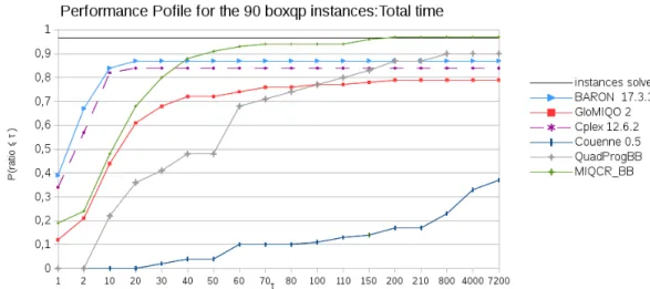
In these experiments, we set the time limit to 1 hour, and we set the node selection strategy to ”best first”. In Figure 1, we present the performance pro-file [28] of the CPU times for methodsMIQCR BB,QuadprogBB,Cplex,Couenne,
BARON andGloMIQOover the 90boxqp instances. In this profile we can see that
MIQCR BBoutperforms the other algorithms both in terms of the total CPU time and of the number of instances solved. We do not report results for the solver
Scipas it was less efficient than Couenne. More precisely, it solves 17 instances out of 90 within the time limit.
Fig. 1.Performance profile of the total time for the boxqpinstances with n= 20 to 100 with a time limit of 1 hour.
In Tables 1 and 2 we present a more detailed comparison. Each line corre-sponds to one instance. We report in ColumnGapthe initial gap that is equal to
|Opt−Bound
Opt |∗100 whereOptis the best known solution of the instance andBound
the optimal value of the relaxation at the root node of the branch-and-bound, in Column Time the CPU time in seconds, where -means that the instance is unsolved within the time limit, and in ColumnNodes the number of nodes vis-ited. For these instances, the initial gaps of methodsMIQCR BBandQuadProgBB
are the same, while the initial gap of Cplex is about 105 times larger. We did not report the reformulation time, but we observe that inMIQCR BBthe reformu-lation phase represents about 32% of the total solution time, and it represents about 3.6% forQuadProgBB.
For these instances,Couenneis not able to solve instances with more than 60 variables within the time limit while the other methods solve instances with up to 100 variables within one hour. We observe that the complete linearization used in Couenne is outperformed by MIQCR BBas suggested by Corollary 1. Finally, over the 90 considered instances,Couennesolves 33 instances,GloMIQOsolves 71 instances (with a relative gap of 10−4instead of 10−5for other methods),Cplex
solves 76 instances,BARON solves 78 instances,QuadProgBBsolves 81 instances, andMIQCR BBsolves 87 instances within the time limit. In particularMIQCR BBis more performant for large instances with high density.
In Table 3, we report the results of MIQCR BBandCplexfor the 9 instances of boxqp with n = 125. We observe that MIQCR BB is able to solve one more instance, butCplexis faster over the 2 instances solved by both methods.
5.2 Instances of quadratically constrained quadratic programs :
IQCP5 and QCP5
We use classIQCP5from [17] and we build classQCP5by continous relaxation
of the variables of IQCP5. Each instance consists of minimizing a quadratic
function subject to 5 quadratic inequality constraints. Instances ofIQCP5were
randomly generated as follows:
– `i= 0 andui= 20, for alli∈I={1, . . . , n}.
– The coefficients ofQ0are integers uniformly distributed in the interval [−5,5]
with a density of 75%, andc0= 0
– The coefficients ofQrare integers uniformly distributed in the interval [0,10]
with a density of 25%, andcr= 0
– br=b0.1∗( n X i=1 n X j=1 qrijuiuj)c.
We use the instances with n= 10, 20, 30, 40 or 50 for each class, and for each n we have 10 instances. We have a total of 100 instances. The instances are named QCP5-n-k or IQCP5-n-k where n is the number of variables, and k is the instance number.
In these experiments, we set the time limit to 1 hour, and we set the node selection strategy to ”best first” for QCP5 and to ”depth first” forIQCP5. In
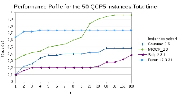
Fig. 2.Performance profile of the total time for theQCP5 instances withn = 10 to
50 with a time limit of 1 hour.
Fig. 3.Performance profile of the total time for theIQCP5 instances withn= 10 to
MIQCR BB,Couenne, Scip, andBARON over the 50QCP5 instances, and in
Fig-ure 3 for the 50IQCP5 instances. We recall that the difference between classes
QCP5 andIQCP5 is only the type of the variables. InQCP5 all variables are
continuous, while in IQCP5 they are all integers. In these profiles, for both
classes, we observe that MIQCR BBoutperforms the other algorithms.
We present in Tables 4–7 a more detailed comparison of the methods. Each line corresponds to one instance. We report in ColumnSdp T.the reformulation CPU time, and in ColumnsBB T.the time spent for the sBB. In Table 4, we can observe thatBARONis the fastest solver for the smallest instances andMIQCR BBis the fastest solver for the largest instances. Moreover, for instances withn= 40,
BARONsolves 7 instances over 10 within the time limit, whileMIQCR BBsolves the 10 instances. In Table 6, we observe that thatCouenneis fastest for the smallest instances (n= 10 or 20), and here again, MIQCR BBis the fastest solver for the largest instances (n = 30 or 40). Indeed, MIQCR BB solves all these instances, whileCouennesolves 5 out of 20,BARONsolves 3 out of 20, andScipis not able to solve any instances of these sizes.
We observe that the initial gap with reformulation (P∗) (S0=S0∗:MIQCR BB)
is on average about 15 times smaller than the initial gap with the complete linearization (S0 =0n: Couenne) for these instances. It is important to notice
that the sizes of the two reformulations are the same. However, the price of this better initial gap is the solution of a semi-definite relaxation. In fact this solution time represents about 38% of the total time on average over the 100 instances.
The results for the 10 generated instances of each class QCP5 and IQCP5
withn= 50 are reported in Tables 5 and 7.MIQCR BBis able to solve 8 instances of class QCP5 and 4 of class IQCP5 while Couenne, Scip, and BARON cannot
solve any one. We also tested mixed-integer instances built from IQCP5 where
we relax the integrality constraints of half of the variables. Since the results reveal a similar trend as for instances of classesQCP5 andIQCP5, we did not
report the specific results in this section.
5.3 Results for the unitbox instances
Each instance from [8] consists in minimizing a quadratic function ofn contin-uous variables in the interval [0,1], subject tomquadratic inequalities. For the considered instances,nvaries from 8 to 50, andmfrom 8 to 100. An instance is denoted byunitbox-n-m-k-dwherenis the number of variables,mis the number of quadratic constraints,kis the instance number, anddis the density in %. We set the time limit to 2 hours, and the node selection strategy to ”best first”.
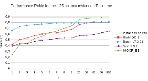
In Figure 4, we present the performance profile of the CPU times for meth-ods MIQCR BB, GloMIQO, Scip, and BARON over the 135 unitbox instances. We observe that MIQCR BBoutperforms the other methods. Here again, the results forGloMIQOare taken from [48].
In Tables 8-10, we present a more detailed comparison of the methods. Each line corresponds to one instance. We observe that Scip solves 88 instances,
Fig. 4.Performance profile of the total time for the unitboxinstances withn= 8 to 50 with a time limit of 2 hours.
of 135 within the time limit. Observe thatGloMIQOorBARONare faster on most of the sparse instances, whileMIQCR BBis again faster on large and dense instances.
6
Conclusion
We consider the general problem (P) of minimizing a quadratic function subject to quadratic constraints where the variables can be integer or continuous. In this paper, we extend the quadratic convex reformulation method to the solution of (P). Our previous versions of this method could handle these programs with the restriction that all quadratic sub-functions of purely continuous variables are already convex.
We start by a reformulation step which solves a semidefinite program (SDP) in order to build an equivalent quadratic program. From this equivalent program, we compute a strong quadratic convex relaxation which captures the tightness of (SDP). In previous versions, in the presence of continuous variables, the reformu-lated problem was computed thanks to a weaker semidefinite relaxation of (P), but it could be solved by standard branch-and-bound for mixed-integer quadratic convex programs. In this paper, to handle the continuous variable case, we build a tighter convex relaxation, but we can no longer rely on standard branch-and-bound. We thus develop an appropriate spatial branch-and-bound to solve the reformulated problem where the bounding step solves our strong quadratic
con-vex relaxation. Our whole method can be viewed as an improvement of the classic spatial branch-and-bound based on complete linearization.
We report computational results on 325 instances. These results show that the method allows us to solve almost all the continuous box-constrained instances with up to 100 variables and some of the instances with 125 variables. Among the considered instances with 5 inequality constraints, the method can handle instances with up to 50 integer or continous variables in less than 1 hours of computation time. Finally, for the unitbox instances, our method solves 119 instances out of 135 within a time limit of 2 hours, which is, to the best of our knowledge, the best result for this class of problems.
Acknowledgement:This research was partially funded by the Fondation Math´ematique Jacques Hadamard (FMJH) through the Gaspard Monge Pro-gram for Optimization and operations research (PGMO). The authors are grate-full to Alain Billionnet for all our collaborations and for a caregrate-full reading of this manuscript.
References
1. T. Achterberg. Scip : solving constraint integer programs.Mathematical Program-ming Computation, (1):1–41, 2009.
2. Claire S Adjiman, Ioannis P Androulakis, and Christodoulos A Floudas. A global optimization method,αbb, for general twice-differentiable constrained nlpsii. im-plementation and computational results. Computers & Chemical Engineering, 22(9):1159–1179, 1998.
3. C.S. Adjiman, S. Dallwig, C.A. Floudas, and A. Neumaier. A global optimiza-tion method, αbb, for general twice-differentiable constrained nlpsi. theoretical advances. Computers and Chemical Engineering, 22(9):1137–1158, 1998.
4. I.P. Androulakis, C.D. Maranas, and C.A. Floudas. abb : A global optimization method for general con- strained nonconvex problems.Journal of Global Optimiza-tion, 7:337–363, 1995.
5. M.F. Anjos and J.B. Lasserre. Handbook of semidefinite, conic and polynomial optimization: Theory, algorithms, software and applications. International Series in Operational Research and Management Science, 166, 2012.
6. K. M. Anstreicher. Semidefinite programming versus the reformulation-linearization technique for nonconvex quadratically constrained quadratic pro-gramming. Journal of Global Optimization, 43(2):471–484, 2009.
7. C. Audet, J. Brimberg, P. Hansen, S. Le Digabel, and N. Mladenovi´c. Pool-ing problem: Alternate formulations and solution methods. Management science, 50(6):761–776, 2004.
8. X. Bao, N. V. Sahinidis, and M. Tawarmalani. Multiterm polyhedral relaxations for nonconvex, quadratically constrained quadratic programs. Optimization Methods Software, 24(4-5):485–504, 2009.
9. X. Bao, N.V. Sahinidis, and M. Tawarmalani. Semidefinite relaxations for quadrat-ically constrained quadratic programming: A review and comparisons. Mathemat-ical Programming, 129:129–157, 2011.
10. P. Belotti, C. Kirches, S. Leyffer, J. Linderoth, J. Luedtke, and A. Mahajan. Mixed-integer nonlinear optimization. Acta Numerica, 22:1–131, 2013.
11. P. Belotti, J. Lee, L. Liberti, F. Margot, and A. Waechter. Branching and bounds tightening techniques for non-convex minlp. Optimization Methods and Software, 4–5(24):597–634, 2009.
12. A. Billionnet. Optimisation discr`ete, De la mod´elisation `a la r´esolution par des logiciels de programmation math´ematique. Dunod, 2007.
13. A. Billionnet and S. Elloumi. Using a mixed integer quadratic programming solver for the unconstrained quadratic 0-1 problem. Mathematical Programming, 109(1):55–68, 2007.
14. A. Billionnet, S. Elloumi, and A. Lambert. Linear reformulations of integer quadratic programs. InMCO 2008, september 8-10, pages 43–51, 2008.
15. A. Billionnet, S. Elloumi, and A. Lambert. Extending the QCR method to the case of general mixed integer program. Mathematical Programming, 131(1):381– 401, 2012.
16. A. Billionnet, S. Elloumi, and A. Lambert. A branch and bound algorithm for general mixed-integer quadratic programs based on quadratic convex relaxation.
Journal of Combinatorial Optimization, 2(28):376–399, 2014.
17. A. Billionnet, S. Elloumi, and A. Lambert. Exact quadratic convex reformulations of mixed-integer quadratically constrained problems. Mathematical Programming, 158(1):235–266, 2016.
18. A. Billionnet, S. Elloumi, A. Lambert, and A. Wiegele. Using a conic bundle method to accelerate both phases of a quadratic convex reformulation. To appear, Informs Journal On Computing, pages 1–15, 2016.
19. A. Billionnet, S. Elloumi, and M. C. Plateau. Improving the performance of stan-dard solvers for quadratic 0-1 programs by a tight convex reformulation: The QCR method. Discrete Applied Mathematics, 157(6):1185 – 1197, 2009. Reformulation Techniques and Mathematical Programming.
20. C. Bliek, P. Bonami, and A. Lodi. Solving Mixed-Integer Quadratic Programming problems with IBM-CPLEX: a progress report. InProceedings of the Twenty-Sixth RAMP Symposium, Hosei University, Tokyo, October 16-17, 2014.
21. P. Bonami, L. Biegler, A. Conn, G. Cornu´ejols, I. Grossmann, C. Laird, J. Lee, A. Lodi, F. Margot, N. Sawaya, and A. Waechter. An Algorithmic Framework for Convex Mixed Integer Nonlinear Programs. Discrete Optimization, 5(2):186–204, 2008.
22. P. Bonami, O. G¨unl¨uk, and J. Linderoth. Solving box-constrained nonconvex quadratic programs. optimization online, 2016.
23. B. Borchers. CSDP, A C Library for Semidefinite Programming. Optimization Methods and Software, 11(1):613–623, 1999.
24. Fani Boukouvala, Ruth Misener, and Christodoulos A Floudas. Global optimiza-tion advances in mixed-integer nonlinear programming, minlp, and constrained derivative-free optimization, cdfo. European Journal of Operational Research, 252(3):701–727, 2016.
25. S. Burer and A. Letchford. Non-convex mixed-integer nonlinear programming: a survey. Surveys in Oper. Res. and Mgmt. Sci., 17(2):97–106, 2012.
26. S. Burer and D. Vandenbussche. Globally solving box-constrained nonconvex quadratic programs with semidefinite-based finite branch-and-bound.Comput Op-tim Appl, 43:181–195, 2009.
27. J. Chen and S. Burer. Globally solving nonconvex quadratic programming prob-lems via completely positive programming. Mathematical Programming Computa-tion, 4(1):33–52, 2012.
28. D. Dolan and J. Mor´e. Benchmarking optimization software with performance profiles. Mathematical Programming, 91:201–213, 1986.
29. F. Domes and A. Neumaier. Constraint propagation on quadratic constraints.
Constraints, 15(3):404–429, 2010.
30. M. A. Duran and I. E. Grossmann. A mixed-integer nonlinear programming algo-rithm for process systems synthesis. AIChE J, 32(4):592–606, 1986.
31. M. A. Duran and I. E. Grossmann. An outer-approximation algorithm for a class of mixed-integer nonlinear programs. Mathematical Programming, 36:307–339, 1986. 32. J.E. Falk and R.M. SolandErkut. An algorithm for separable nonconvex
program-ming problems. Management Science, 15:550–560, 1969.
33. CA Floudas and CE Gounaris. A review of recent advances in global optimization.
Journal of Global Optimization, 45(1):3–38, 2009.
34. Christodoulos A Floudas and V Visweswaran. A global optimization algorithm (gop) for certain classes of nonconvex nlpsi. theory. Computers & chemical engi-neering, 14(12):1397–1417, 1990.
35. Christodoulos A Floudas and Vishy Visweswaran. Primal-relaxed dual global opti-mization approach. Journal of Optimization Theory and Applications, 78(2):187– 225, 1993.
36. R. Fortet. L’alg`ebre de Boole et ses Applications en Recherche Op´erationnelle.
Cahiers du Centre d’Etudes de Recherche Op´erationnelle, 4:5–36, 1959.
37. M.R. Garey and D.S. Johnson. Computers and Intractability: A guide to the theory of NP-Completness. W.H. Freeman, San Francisco, CA, 1979.
38. W.W. Hager and J.T. Hungerford. Continuous quadratic programming formula-tions of optimization problems on graphs. European Journal of Operational Re-search, 240(2):328 – 337, 2015.
39. P. L. Hammer and A.A. Rubin. Some remarks on quadratic programming with 0-1 variables.Revue Fran¸caise d’Informatique et de Recherche Op´erationnelle, 4:67–79, 1970.
40. C.A. Haverly. Studies of the behaviour of recursion for the pooling problem. ACM SIGMAP Bulletin, 26, 1978.
41. C. Helmberg. Conic Bundle v0.3.10, 2011.
42. IBM-ILOG. IBM ILOG CPLEX 12.6.2 Reference Manual, 2015.
43. A. Lambert. IQCP/MIQCP: Library of Integer and Mixed-Integer Quadratic Quadratically Constrained Programs. ”http://cedric.cnam.fr/~lamberta/
Library/iqcp_miqcp.html”, 2013.
44. M. Madani and M. Van Vyve. Computationally efficient MIP formulation and algorithms for european day-ahead electricity market auctions. European Journal of Operational Research, 242(2):580 – 593, 2015.
45. G.P. McCormick. Computability of global solutions to factorable non-convex pro-grams: Part i - convex underestimating problems. Mathematical Programming, 10(1):147–175, 1976.
46. R. Misener and C. A. Floudas. Global optimization of mixed-integer quadratically-constrained quadratic programs (MIQCQP) through piecewise-linear and edge-concave relaxations. Math. Program. B, 136(1):155–182, 2012. http://www. optimization-online.org/DB_HTML/2011/11/3240.html.
47. R. Misener and C. A. Floudas. GloMIQO: Global mixed-integer quadratic opti-mizer. Journal of Global Optimization, 57(1):3–50, 2013.
48. R. Misener, J. B. Smadbeck, and C. A. Floudas. Dynamically generated cutting planes for mixed-integer quadratically constrained quadratic programs and their incorporation into GloMIQO 2. Optimization Methods and Software, 30(1):215– 249, 2015.
49. J.J. Mor´e and G. Toraldo. Algorithms for bound constrained quadratic program-ming problems. Numerische Mathematik, 55(4):377–400, 1989.
50. M. Kilin¸c P. Bonami and J. Linderoth. Algorithms and software for convex mixed integer nonlinear programs. InMixed integer nonlinear programming, pages 1–39. Springer New York, 2012.
51. N.V. Sahinidis and M. Tawarmalani. Baron 9.0.4: Global optimization of mixed-integer nonlinear programs. User’s Manual, 2010.
52. A. Saxena, P. Bonami, and J. Lee. Convex relaxations of non-convex mixed in-teger quadratically constrained programs: projected formulations. Mathematical Programming, 130:359–413, 2011.
53. H. D. Sherali and W. P. Adams. A hierarchy of relaxation between the continuous and convex hull representations for zero-one programming problems.SIAM Journal Discrete Mathematics, 3:411–430, 1990.
54. M. Tawarmalani and N. V. Sahinidis. Global optimization of mixed-integer nonlin-ear programs: A theoretical and computational study.Mathematical programming, 99(3):563–591, 2004.
55. M. Tawarmalani and N.V. Sahinidis. Convexification and global optimization in continuous and mixed-integer nonlinear programming. Kluwer Academic Publish-ing, Dordrecht, The Netherlands, 2002.
56. M. Tawarmalani and N.V. Sahinidis. A polyhedral branch-and-cut approach to global optimization. Mathematical Programming, 103(2):225–249, 2005.
57. D. Vandenbussche and G. Nemhauser. A branch-and-cut algorithm for nonconvex quadratic programs with box constraints.Mathematical Programming, 102(3):259– 275, 2005.
58. S. Vigerske and A. Gleixner. Scip: Global optimization of mixed-integer nonlinear programs in a branch-and-cut framework. optimization online, 2016.
59. V Visweswaran and CA Floudas. New properties and computational improve-ment of the gop algorithm for problems with quadratic objective functions and constraints. Journal of Global Optimization, 3(4):439–462, 1993.
60. V Visweswaran and CA Floudast. A global optimization algorithm (gop) for certain classes of nonconvex nlpsii. application of theory and test problems. Computers & chemical engineering, 14(12):1419–1434, 1990.
61. K. Zorn and N. V. Sahinidis. Computational experience with applications of bi-linear cutting planes. Industrial & Engineering Chemistry Research, 52(22):7514– 7525, 2013.
62. K. Zorn and N. V. Sahinidis. Global optimization of general non-convex prob-lems with intermediate bilinear substructures.Optimization Methods and Software, 29(3):442–462, 2014.