Mikołaj Bojańczyk
1and Michał Pilipczuk
21 Institute of Informatics, University of Warsaw, Warsaw, Poland
2 Institute of Informatics, University of Warsaw, Warsaw, Poland
Abstract
The classic algorithm of Bodlaender and Kloks [J. Algorithms, 1996] solves the following problem in linear fixed-parameter time: given a tree decomposition of a graph of (possibly suboptimal) widthk, compute an optimum-width tree decomposition of the graph. In this work, we prove that this problem can also be solved inmsoin the following sense: for every positive integerk, there is anmsotransduction from tree decompositions of widthkto tree decompositions of optimum width. Together with our recent results [LICS 2016], this implies that for everyk there exists an msotransduction which inputs a graph of treewidthk, and nondeterministically outputs its tree decomposition of optimum width.
1998 ACM Subject Classification F.4.3 Formal Languages, G.2.2 Graph Theory
Keywords and phrases tree decomposition, treewidth, transduction, monadic second-order logic
Digital Object Identifier 10.4230/LIPIcs.STACS.2017.15
1
Introduction
Consider the following problem: given a tree decomposition of a graph of some width k, possibly suboptimal, we would like to compute an optimum-width tree decomposition of the graph. A classic algorithm of Bodlaender and Kloks [4] solves this problem in linear fixed-parameter time complexity, where the input widthkis the parameter.
ITheorem 1(Bodlaender and Kloks, [4]). There exists an algorithm that, given a graph G
onnvertices and its tree decomposition of widthk, runs in time2O(k3)·nand returns a tree
decomposition ofGof optimum width.
The algorithm of Bodlaender and Kloks proceeds by a bottom-up dynamic programming procedure on the input decomposition. For every subtree, a set of partial optimum-width decompositions is computed. The crucial ingredient is a combinatorial analysis of partial decompositions which shows that only some small subset of them, of size bounded only by a function ofk, needs to be remembered for future computation.
The algorithm of Bodlaender and Kloks is a key subroutine in the linear-time algorithm for computing the treewidth of a graph, due to Bodlaender [2]. The fact that the algorithm is essentially governed by a run of a finite-state automaton on the input tree decomposition was also used in the recent approximation algorithm of Bodlaender et al. [3]. The notion of
∗ A full version of the paper is available athttps://arxiv.org/abs/1701.06937.
† The research of M. Bojańczyk is supported by the European Research Council (ERC) under the European Union’s Horizon 2020 research and innovation programme (ERC consolidator grant LIPA, agreement no. 683080). Mi. Pilipczuk is supported by the Foundation for Polish Science via the START stipend programme.
typical sequences, which is the main component of the analysis of partial decompositions, has found applications in algorithms for computing other width measures, like branchwidth [5], cutwidth [16, 17], or pathwidth of matroids [12]. The concept of typical sequences originates in the previous work of Courcelle and Lagergren [8] and of Lagergren and Arnborg [15].
Our results. The main result of this paper (Theorem 2) is that the problem of Bodlaender and Kloks can be solved by anmsotransduction, which is a way of describing nondeterministic transformations of relational structures using monadic second-order logic. More precisely, we show that for every k ∈ {0,1,2, . . .} there is an mso transduction that inputs a tree decomposition of widthkof a graphG, and outputs nondeterministically a tree decomposition ofGof optimum width.
As a corollary of our main result, we show (Corollary 3) that anmsotransduction can compute an optimum-width tree decomposition, even if the input is only the graph and not a (possibly suboptimal) tree decomposition. This application is obtained by combining the main result of this paper with Theorem 2.4 from [6], which says that for everyk∈ {0,1,2, . . .}there is anmsotransduction which inputs a graph of treewidthkand outputs nondeterministically one of its tree decompositions of possibly suboptimal width at mostf(k), for some functionf. In particular, we thus strengthen Theorem 2.4 of [6] by making the output a decomposition of exactly the optimum width, instead of only bounded by a function of the optimum.
Our proof is divided into a few steps. First, we prove a result called theDealternation Lemma, which shows that there always exists an optimum-width tree decomposition that has bounded “alternation” with respect to the input suboptimal decomposition. Intuitively, small alternation is the key property allowing an optimum-width tree decomposition to be captured by anmsotransduction or by a dynamic programming algorithm that works on the input suboptimal decomposition. This part of the proof essentially corresponds to the machinery of typical sequences of Bodlaender and Kloks. However, we find the approach via alternation more intuitive and combinatorially less complicated, and we hope that it will find applications for computing other width measures. In fact, a similar approach has very recently been used by Giannopoulou et al. [10] in a much simpler setting of cutwidth to give a new fixed-parameter algorithm for this graph parameter.
Next, we derive a corollary of the Dealternation Lemma called the Conflict Lemma, which directly prepares us to construct the mso transduction for the Bodlaender-Kloks problem. The Conflict Lemma is stated in purely combinatorial terms, but intuitively it shows that some optimum-width tree decomposition of the graph can be interpreted in the given suboptimum-width tree decomposition using subtrees that cross each other in a restricted fashion, guessable inmso. Finally, we formalize the intuition given by the Conflict Lemma inmso, thus constructing themso transduction promised in our main result.
2
Preliminaries and statement of the main result
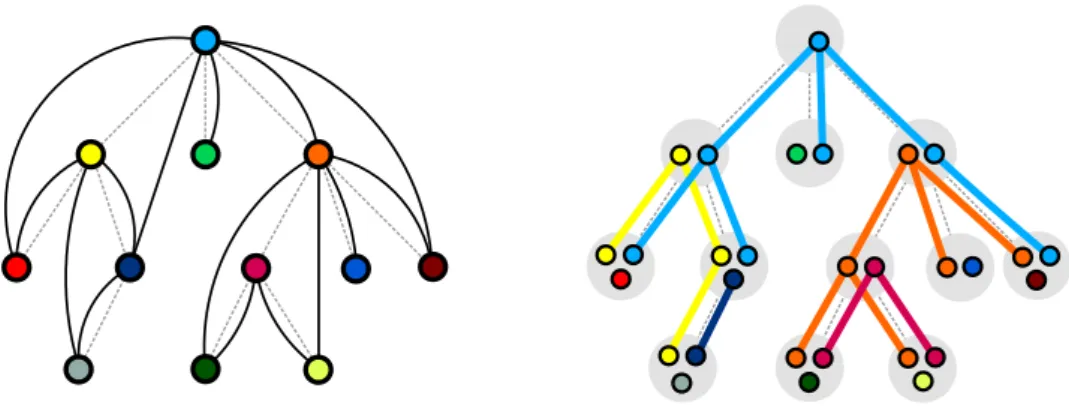
Trees, forests and tree decompositions. Throughout this paper all graphs are undirected, unless explicitly stated. Aforest(which is sometimes called arooted forest in other contexts) is defined to be an acyclic graph, where every connected component has one designated node called theroot. This naturally imposes parent–child and ancestor–descendant relations in a (rooted) forest. We use the usual tree terminology: root, leaf, child, parent, descendant and ancestor. We assume that every node is its own descendant, to exclude staying in the same node we use the namestrict descendant. Likewise for ancestors. For forests we often use the namenodeinstead of vertex. A tree is the special case of a forest that is connected and thus
has one root. Two nodes in a forest are called siblings if they have a common parent, or if they are both roots. Note that there is no order on siblings, unlike some models of unranked trees and forests where siblings are ordered from left to right.
A tree decompositionof a graphGis a pairt= (F, β), whereF is a rooted forest andβ is a function that associatesbags to the nodes ofF.A bag is a nonempty subset of vertices of G. We require the following two properties:
(T1) whenever uvis an edge ofG, then there exists a node ofF whose bag contains bothu and v; and
(T2) for every vertex uofG, the set of nodes ofF whose bags contain uis nonempty and induces a connected subtree in F.
Thewidth of a tree decomposition is its maximum bag size minus 1, and thetreewidth of a graph is the minimum width of its tree decomposition. Anoptimum-widthtree decomposition is one whose width is equal to the treewidth of the underlying graph. Note that throughout this paper all tree decompositions will be rooted forests. This slightly diverges from the literature where usually the shape of a tree decomposition is an unrooted tree.
For a tree decompositiont= (F, β) of a graphG, and each nodexofF, we define the following vertex sets:
The adhesion of x, denoted σ(x), is equal to β(x)∩β(x0), wherex0 is the parent ofx in F. Ifxis a root ofF, we define its adhesion to be empty.
Themargin ofx, denotedµ(x), is equal toβ(x)\σ(x).
Thecomponent ofx, denotedα(x), is the union of the margins of all the descendants of x(includingxitself). Equivalently, it is the union of the bags of all the descendants ofx, minus the adhesion ofx.
Whenever the tree decompositiontis not clear from the context, we specify it in the subscript, i.e., we use operatorsβt(·),σt(·),µt(·), andαt(·).
Observe that, by property (T2) of a tree decomposition, for every vertex ofGthere is a unique node whose bag containsu, but the bag of its parent (if exists) does not containu. In other words, there is a unique node whose margin containsu. Consequently, the margins of the nodes of a tree decomposition form a partition of the vertex set of the underlying graph.
Relational structures and MSO. Define avocabulary to be a finite set ofrelation names, each with associated arity that is a nonnegative integer. A relational structure over the vocabulary Σ consists of a set called theuniverse, and for each relation name in the vocabulary, an associated relation of the same arity over the universe. To describe properties of relational structures, we use logics, mainly monadic second-order logic (mso for short). This logic allows quantification both over single elements of the universe and also over subsets of the universe. For a precise definition ofmso, see [7].
We use msoto describe properties of graphs and tree decompositions. To do this, we need to model graphs and tree decompositions as relational structures. A graph is viewed as a relational structure, where the universe is a disjoint union of the vertex set and the edge set of a graph. There is a single binary incidence relation, which selects a pair (v, e) whenever v is a vertex and e is an incident edge. The edges can be recovered as those elements of the universe which appear on the second coordinate of the incidence relation; the vertices can be recovered as the rest of the universe. For a tree decomposition of a graph G, the universe of the corresponding structure consists of the disjoint union of: the vertex set of G, the edge set ofG, and the node set of the tree decomposition. There is the incidence relation between vertices and edges, as for graphs, a binary descendant relation over the nodes of the tree decomposition, and a binary bag relation which selects pairs (v, x) such that xis
a node of the tree decomposition whose bag contains vertexv of the graph. The nodes of the decomposition can be recovered as those which are their own descendants, since we assume that the descendant relation is reflexive. Note that thus, the representation of a tree decomposition as a relational structure contains the underlying graph as a substructure.
MSO transductions. Suppose that Σ and Γ are vocabularies. Define atransduction with input vocabulary Σ and output vocabulary Γ to be a set of pairs
(input structure over Σ, output structure over Γ)
which is invariant under isomorphism of relational structures. When talking about transduc-tions on graphs or tree decompositransduc-tions, we use the representatransduc-tions described in the previous paragraph. Note that a transduction is a relation and not necessarily a function, thus it can have many different possible outputs for the same input. A transduction is called determ-inisticif it is a partial function (up to isomorphism). For example, the subgraph relation is a transduction from graphs to graphs, but it is not deterministic since a graph can have many subgraphs. On the other hand, the transformation that inputs a tree decomposition and outputs its underlying graph is a deterministic transduction.
This paper usesmsotransductions, as defined in the book of Courcelle and Engelfriet [7], which are a special case of transductions that can be defined using the logic mso. The precise definition is in Section 5, but the main idea is that anmsotransduction is a finite composition of transductions of the following types: copy the input a fixed number of times, nondeterministically color the universe of the input, and add new predicates to the vocabulary with interpretations given bymsoformulas over the input vocabulary. We refer to Courcelle and Engelfriet [7] for a broader discussion of the role ofmsotransduction in the theory of formal languages for graphs.
The main result. We now state the main contribution of this paper, which is an mso version of the algorithm of Bodlaender and Kloks.
ITheorem 2. For everyk∈ {0,1,2, . . .} there is anmsotransduction from tree decomposi-tions to tree decomposidecomposi-tions such that for every input tree decomposition t:
if thas width at mostk, then there is at least one output; and
every output is an optimum-width tree decomposition of the underlying graph oft.
We remark that the transduction of Theorem 2 is not deterministic, i.e. it might have several outputs on the same input. Using Theorem 2, we prove that an mso transduction can compute an optimum-width tree decomposition given only the graph.
ICorollary 3. For every k∈ {0,1,2, . . .}there is anmsotransduction from graphs to tree decompositions such that for every input graph G:
if Ghas treewidth at mostk, then there is at least one output; and every output is a tree decomposition ofGof optimum width.
Proof. Theorem 2.4 of [6] says that for everyk∈ {0,1,2, . . .} there is anmso transduction with exactly the properties stated in the statement, except that when the input has treewidth k, then the output tree decompositions have width at mostf(k), for some functionf:N→N.
By composing this transduction with the transduction given by Theorem 2, applied tof(k),
Structure of the paper. The rest of this paper is devoted to the proof of Theorem 2. In Section 3 we formulate the Dealternation Lemma. Intuitively, this result says that any optimum-width tree decompositionscan be adjusted without increasing the width so that it behaves nicely with respect to the input suboptimal decompositiont in the following sense: for every subtree oft, the vertices appearing in the bags of this subtree are partitioned into few “connected blocks” in s. This part holds the essence of typical sequences of Bodlaender and Kloks [4], but in the full version of the paper (seehttps://arxiv.org/abs/1701.06937) we give a self-contained proof in order to achieve stronger assertions and highlight the key combinatorial properties we use later on. Then, we prove a corollary of the Dealternation Lemma, which we call the Conflict Lemma. This result intuitively states that some optimum-width tree decomposition of the graph can be interpreted in the given suboptimum-optimum-width tree decomposition. This intuition is formalized in the last section, where we introduce formally msotransductions and use the combinatorial property given by the Conflict Lemma to prove Theorem 2.
3
Dealternation
This section is devoted to the Dealternation Lemma, which intuitively says that for a tree decomposition t of bounded, though possibly suboptimal width, there always exists an optimum-width decomposition in which every subtree oftis broken into small number of “pieces”. We begin by defining factors, which is our notion of “pieces” of a tree decomposition.
Factors and factorizations. Intuitively, a factor is a set of nodes in a forest that respects the tree structure. We define three kinds of factors: tree factors, forest factors, and context factors. Atree factor in a forest is a set of nodes obtained by taking all (not necessarily strict) descendants of some node, which is called theroot of the tree factor. Define a forest factor to be a nonempty union of tree factors whose roots are siblings. These roots are called theroots of the forest factor. In particular, a tree factor is also a forest factor, with one root.
X
roots of the forest factor outside the forest factor non-roots of the forest factor
X Y
root of the context factor appendices of the context factor
outside the context factor non-roots of the context factor
a forest factor a context factor
A context factor is the difference X−Y for a tree factorX and a forest factor Y, where the root of X is a strict ancestor of every root of Y. For a context factorX−Y, its root is defined to be the root ofX, while the roots ofY are called the appendices. Note that a context factor always contains a unique node that is the parent of all its appendices.
Forest factors and context factors will be jointly calledfactors. The following lemma can be proved by a straightforward case study, and hence we leave its proof to the reader. ILemma 4. The union of two intersecting factors in the same forest is also a factor.
For a subsetU of nodes of a forest, aU-factor is a factor that is entirely contained inU. A factorizationof U is a partition ofU intoU-factors. AU-factor is maximal if no other U-factor contains it as a strict subset.
I Lemma 5. For every subset of nodes U in a forest, the maximal U-factors form a factorization ofU.
Proof. Every node ofU is contained in some factor, e.g., a singleton factor (which has forest
or context type depending on whether the node is a leaf or not). Thus, every node ofU is also contained in some maximal U-factor. On the other hand, two different maximal U-factors must be disjoint, since otherwise by Lemma 4, their union would also be aU-factor,
contradicting maximality. J
The set of all maximalU-factors will be called themaximal factorizationofU, and will be denoted byfact(U). We specify the forest in the subscript whenever it is not clear from the context. Lemma 5 asserts thatfact(U) is indeed a factorization ofU. Note that the maximal factorization ofU is the coarsest in the following sense: in every factorization ofU, each of its factors is contained in some factor offact(U). In particular, the maximal factorization has the smallest number of factors among all factorizations ofU.
In the sequel, we will need the following simple result about relation between the maximal factorizations of a set and of its complement. Its proof is a part of the proof of the Dealternation Lemma, and can be found in the full version of the paper.
ILemma 6. Suppose(U, W)is a partition of the node set of a rooted forestF, and letkbe the number of factors in the maximal factorization of W. Then the maximal factorization of
U has at mostk+ 1 forest factors and at most 2k−1 context factors.
Separation forests. The general definition of a tree decomposition is flexible and allows for multiple combinatorial adjustments. Here, we will rely on a normalized form that we callseparation forests, which are essentially tree decompositions where all the margins have size exactly 1. The definition of treewidth via separation forests resembles the definition of pathwidth via the so-calledvertex separation number [14].
IDefinition 7. SupposeGis a graph. Aseparation forest ofGis a rooted forestF on the same vertex set asGsuch thatGis contained in the ancestor-descendant closure ofF; that is, wheneveruv is an edge ofG, thenuis an ancestor ofv inF or vice versa.
Separation forests are used to define the graph parametertreedepth, which is equal to the minimum depth of a separation forest of a graph. To define treewidth, we need to take a different measure than just the depth, as explained next.
SupposeF is a separation forest of G. Endow F with the following bag functionβ(·). For any vertexuofG, assign touthe bagβ(u) consisting ofuand all the ancestors ofuin F that have a neighbor among the descendants of uinF. The following claim follows by verifying the definition of a tree decomposition; we leave the easy proof to the reader. IClaim 8. IfF is a separation forest ofGandβ(·)is defined as above, then(F, β)is a tree decomposition of G. Moreover, for every vertexuofG, the margin ofuin(F, β)is{u}.
The tree decomposition (F, β) defined above is said to be induced by the separation forestF. Observe that ift= (F, β) is induced byF, then for any vertex u, the component ofuin tconsists of all the descendants ofuinF.
Figure 1Construction of the induced tree decomposition from a separation forest. The graph edges are depicted in black, the child-parent relation of the forest is depicted as dashed grey lines.
One can reformulate the construction given above as follows. First, put every vertex u into its bagβ(u). Then, examine every neighborvof u, and ifv is a descendant ofuinF, then adduto every bag on the path fromv touinF. Thus, every vertexuis “smeared” onto a subtree of F, whereuis the root of this subtree and its leaves correspond to those neighbors ofuthat are also its descendants inF. This construction is depicted in Figure 1.
Thewidth of a separation forest is simply the width of the tree decomposition induced by it. Consequently, the width of a separation forest is never smaller than the treewidth of a graph. The next result shows that in fact there is always a separation forest of optimum width. The proof follows by a simple surgery on an optimum-width tree decomposition, and can be found in the full version of the paper.
ILemma 9. For every graphGthere exists a separation forest ofGwhose width is equal to the treewidth ofG.
Dealternation Lemma. We are finally ready to state the Dealternation Lemma.
ILemma 10(Dealternation Lemma). There exist functions f(k)∈ O(k2)and g(k)∈ O(k3)
such that the following holds. Suppose thatt is a tree decomposition of a graphGof width k. Then there exists an optimum-width separation forestF ofGsuch that:
(D1) for every node xoft, the maximal factorizationfactF(αt(x))has at mostf(k)factors;
(D2) for every node xoft, there are at most g(k)children of xin the set
{y:y is a node of t with at least one context factor infactF(αt(y))}.
Note that in the statement of the Dealternation Lemma, the vertex set of Gis at the same time the node set of the forestF. Thus,factF(αt(x)) denotes the maximal factorization
ofαt(x), treated as a subset of nodes ofF.
The proof of the Dealternation Lemma uses essentially the same core ideas as the correctness proof of the algorithm of Bodlaender and Kloks [4]. We include our proof in the full version of the paper for several reasons. First, unlike in [4], in our setting we cannot assume that t has binary branching, as is the case in [4]. In fact, condition (D2) is superfluous whenthas binary branching. Second, our formulation of the Dealternation Lemma highlights the key combinatorial property, which is expressed as the existence of a single separation forestF that behaves nicely with respect to the input decompositiont. This property is somehow implicit [4], where the existence of nicely-behaved optimum-width tree decompositions is argued along performing dynamic programming. For this reason, we find the new formulation more explanatory and potentially interesting on its own.
4
Using the Dealternation Lemma
In this section we use the Dealternation Lemma to show that an optimum-width separation forest of a graph can be interpreted in a suboptimum-width tree decomposition. For this, we need to develop a better understanding of the combinatorial insight provided by the Dealternation Lemma, which is expressed via an auxiliary graph, called theconflict graph.
SupposeGis a graph,tis a tree decomposition ofGof widthk, andF is a separation forest ofG. Letφbe the mapping that sends each vertexuofGto the unique node oftthat containsuin its margin. For a vertexuofG, we define thestain ofu, denotedSu, which
is a subgraph of the underlying forest oft, as follows. For every childv ofuinF, find the unique path int betweenφ(u) andφ(v). Then stainSu consists of the nodeφ(u) and the
union of these paths. Note that ifuis a leaf ofF, then the stainSuconsists only of the node
φ(u). Define theconflict graph H(t, F) as follows. The vertices ofH(t, F) are the vertices of G, and vertices uandv are adjacent in H(t, F) if and only their stains Su andSv have a
node in common. The main result of this section can be formulated as follows.
ILemma 11 (Conflict Lemma). There is a functionh(k)∈ O(k5)such that ift andF are as in the Dealternation Lemma, then their conflict graph H(t, F) admits a proper coloring withh(k)colors.
Recall here that a proper coloring of a graph is a coloring of its vertex set such that no two adjacent vertices receive the same color. The rest of this section is devoted to the proof of the Conflict Lemma. From now on, we assume thatG, t, F are as in the Dealternation Lemma, and we denoteH =H(t, F).
Observe that the conflict graphH is an intersection graph of a family of subtrees of a forest. It is well-known (see, e.g., [11]) that this property precisely characterizes the class of chordal graphs (graphs with no induced cycle of length larger than 3), soH is chordal. Chordal graphs are known to be perfect (again see, e.g., [11]), hence the chromatic number of a chordal graph (the minimum number of colors needed in a proper coloring) is equal to the size of the largest clique in it. On the other hand, subtrees of a forest are known to satisfy the so-called Helly property: wheneverF is some family of subtrees such that the subtrees inF pairwise intersect, then in fact there is a node of the forest that belongs to all the subtrees inF. This means that the largest clique in an intersection graph of a family of subtrees of a forest can be obtained by taking all the subtrees that contain some fixed node. Therefore, to prove the Conflict Lemma it is sufficient to prove the following claim.
IClaim 12. There exists a function h(k)∈ O(k5)such that every node oft belongs to at mosth(k)of the stains{Su:u∈V(G)}.
In the remainder of this section we prove Claim 12. Fix any node x of t, and let y1, y2, . . . , yp be its children int. Consider the following partition of the vertex set ofG:
Π = (αt(y1), αt(y2), . . . , αt(yp), µt(x), V(G)\αt(x))
Define a factorization Φ of the whole node set of F as follows: for each setX from the partition Π, take its maximal factorizationfactF(X), and define Φ to be the union of these
maximal factorizations. Thus, Φ is a factorization that refines the partition Π. Since the number of childrenyi is unbounded, we cannot expect that Φ has a small number of factors,
but at least it has a small number of context factors.
IClaim 13. FactorizationΦcontains at mostg(k)·f(k) + 2f(k) +k context factors, where
Proof. By the Dealternation Lemma, the maximal factorization inF of each of the sets αt(y1), . . . , αt(yp), αt(x) has at mostf(k) factors. Moreover, only at mostg(k) of the sets
αt(y1), . . . , αt(yp) can have a context factor in their maximal factorizations. Hence, the
maximal factorizations of setsαt(y1), . . . , αt(yp) introduce at mostg(k)·f(k) context factors
to the factorization Π. Since the maximal factorization ofαt(x) has at mostf(k) factors as
well, by Lemma 6 we deduce that the maximal factorization ofV(G)\αt(x) has at most
2f(k)−1 context factors. Finally, the cardinality ofµt(x) is at mostk+ 1, so in particular
its maximal factorization has at mostk+ 1 factors in total. Summing up all these upper bounds, we conclude that Φ has at mostg(k)·f(k) + 2f(k) +kcontext factors. J With Claim 13 in hand, we complete now the proof of Claim 12. Take any vertex usuch thatxbelongs to the stainSu. This means that either
(i) ubelongs to the margin of x, or
(ii) udoes not belong to the margin ofx, butuhas a child v inF such that the unique path int betweenφ(u) andφ(v) passes throughx.
The number of verticesusatisfying 1 is bounded by the size of the margin ofx, which is at most k+ 1, hence we focus on vertices u that satisfy 2. Observe that condition 2 in particular means thatuandv belong to different parts of partition Π, so also to different factors of factorization Φ. Sinceuis the parent ofv inF, this means that the unique factor of Φ that containsumust be a context factor, andumust be the parent of its appendices. Consequently, the number of vertices usatisfying 2 is upper bounded by the number of context factors in factorization Φ, which is at mostg(k)·f(k) + 2f(k) +k by Claim 13. We conclude that the number of stains Su containingxis at most
h(k) :=g(k)·f(k) + 2f(k) + 2k+ 1;
in particularh(k)∈ O(k5). This concludes the proof of Claim 12, so also the proof of the
Conflict Lemma is complete.
5
Constructing the transduction
We now use the understanding gathered in the previous sections to give anmsotransduction that takes a tree decomposition of a graph of suboptimum width, and produces an optimum-width tree decomposition. First, we need to precisely definemso transductions.
MSO transductions. Formally, an mso transduction is any transduction that can be obtained by composing a finite number of transductions of the following kinds. Note that kind 1 is a partial function, kinds 2, 3, 4 are functions, and kind 5 is a relation.
1. Filtering. For every mso sentenceϕ over the input vocabulary there is transduction that filters out structures whereϕis satisfied. Formally, the transduction is the partial identity whose domain consists of the structures that satisfy the sentence. The input and output vocabularies are the same.
2. Universe restriction. For everymsoformulaϕ(x) over the input vocabulary with one free first-order variable there is a transduction, which restricts the universe to those elements that satisfyϕ. The input and output vocabularies are the same, the interpretation of each relation in the output structure is defined as the restriction of its interpretation in the input structure to tuples of elements that remain in the universe.
3. MSO interpretation. This kind of transduction changes the vocabulary of the structure while keeping the universe intact. For every relation nameRof the output vocabulary,
there is an msoformulaϕR(x1, . . . , xk) over the input vocabulary which has as many
free first-order variables as the arity ofR. The output structure is obtained from the input structure by keeping the same universe, and interpreting each relationR of the output vocabulary as the set of those tuples (x1, . . . , xk) that satisfyϕR.
4. Copying. For k ∈ {1,2, . . .}, define k-copying to be the transduction which inputs a structure and outputs a structure consisting ofkdisjoint copies of the input. Precisely, the output universe consists ofkcopies of the input universe. The output vocabulary is the input vocabulary enriched with a binary predicatecopythat selects copies of the same element, and unary predicateslayer1,layer2, . . . ,layerk which select elements belonging to the first, second, etc. copies of the universe. In the output structure, a relation nameRof the input vocabulary is interpreted as the set of all those tuples over the output structure, where the original elements of the copies were in relationR in the input structure.
5. Coloring. We add a new unary predicate to the input structure. Precisely, the universe as well as the interpretations of all relation names of the input vocabulary stay intact, but the output vocabulary has one more unary predicate. For every possible interpretation of this unary predicate, there is a different output with this interpretation implemented. We remark that the above definition is easily equivalent to the one used in [6], where filtering, universe restriction, andmsointerpretation are merged into one kind of a transduction. Proving the main result. We are finally ready to prove our main result, Theorem 2. The proof is broken down into several steps. The first, main step shows that anmsotransduction can output optimum-width separation forests. Here, a separation forest of a graph G is encoded by enriching the relational structure encoding G with a single binary relation interpreted as the child relation of F. Note that the definition of a separation forest is mso-expressible: there is anmsosentence that checks whether the additional relation indeed encodes a separation forest of the graph.
ILemma 14. For everyk∈ {0,1,2, . . .}, there is an msotransduction from tree decomposi-tions to separation forests such that for every input tree decomposition t:
every output is a separation forest of the underlying graph oft; and
if thas width at most k, then there is at least one output that is a separation forest of optimum width.
Proof. Observe that the verification whether the width oftis at mostkcan be expressed by
anmsosentence, so we can first use filtering to filter out any input tree decompositiont whose width is larger thank; for such decompositions, the transduction produces no output. LetGbe the underlying graph oft, and letφbe the mapping that sends each vertexuofG to the unique node oft whose margin containsu. By the Conflict Lemma, there exists some separation forestF ofGof optimum width such that the conflict graphH(t, F) admits some proper coloringλwithh(k) colors. The constructedmsotransduction attempts at guessing and interpretingF as follows.
First, using coloring and filtering, we guess the coloringλ, represented as a partition of the vertex set ofG. Then, again using coloring and filtering, for every vertexuofGwe guess whetheruis a root ofF, and if not, then we guess the color underλof the parent ofuinF.
Next, for every colorcused inλ, we guess the forest Mc :=
[
u∈λ−1(c) Su,
where Su is the stain of uint, defined as in Section 4 for the separation forest F. Note
the conflict graphH(t, F). Thus, the connected components of Mc are exactly these stains.
Observe also thatMc is a subgraph of the decompositiont, so we can emulate guessing Mc
in anmsotransduction working overtby guessing the subset of those nodes of t, for which the edge oftconnecting the node and its parent belongs to Mc.
Having done all these guesses, we can interpret the child relation of F using anmso predicate as follows. Fix a pair of vertices u andv, and let c be the guessed color of u underλ. Then one can readily check thatuis the parent ofvinF if and only if the following conditions are satisfied:
we have guessed thatv is not a root ofF,
we have guessed that the color of the parent ofv in F isc, and
uis the unique vertex of colorcsuch thatφ(u) belongs to the same connected component ofMc asφ(v).
It can be easily seen that these conditions can be expressed by anmsoformula with two free variablesuandv.
Finally, we filter out all the wrong guesses by verifying, using an msosentence, whether the interpreted child relation on the vertices of Gindeed forms a rooted forest, and whether this forest is a separation forest ofG. Obviously, the separation forestF was obtained for at least one of the guesses, and survives this filtering. At the end, we remove the nodes of decomposition tfrom the structure using universe restriction. J
Next, we need to construct the induced tree decomposition out of a separation forest. ILemma 15. There is anmsotransduction from separation forests to tree decompositions that on each input separation forest has exactly one output, which is the tree decomposition induced by the input.
Proof. We copy the vertex set of the graph two times, and declare the second copies to be the
nodes of the constructed tree decomposition. Using the child relation of the input separation forest, we can interpret inmsothe descendant relation in the forest of the decomposition. Finally, the bag relation in the induced tree decomposition, as defined in Section 3, can be
easily interpreted using anmsoformula. J
Finally, so far the transduction can output tree decompositions of suboptimal width, which should be filtered out. For this, we need the followingmso-expressible predicate. ILemma 16. For everyk∈ {0,1,2, . . .}, there is anmso-sentence over tree decompositions that holds if and only if the given tree decomposition has width at mostk and its width is optimum for the underlying graph.
Proof. Lettbe the given tree decomposition of a graph G. Obviously, we can verify using
an mso sentence whether the width of t is at most k. To check that the width of t is optimum, we could use the fact that graphs of treewidthkare characterized by a finite list of forbidden minors, but we choose to apply the following different strategy. LetRk be themso transduction that is the composition of the transductions of Lemmas 14 (for parameterk) and 15. Provided the input tree decomposition t has width at most k, transduction Rk
outputs some set of tree decompositions ofGamong which one has optimum width. Hence,t has optimum width if and only if the outputRk(t) does not contain any tree decomposition
of width smaller thant.
The Backwards Translation Theorem for msotransductions [7] states that whenever T is anmsotransduction andψis anmsosentence over the output vocabulary, then the set of structures on whichT outputs at least one structure satisfyingψ, is mso-definable over
the input vocabulary. Hence, for everyp < k, there exists anmsosentenceϕp that verifies
whether Rk(t) outputs at least one tree decomposition of width at mostp. Therefore, we
can check whetherthas optimum width by making a disjunction over all` with 0≤`≤k of the sentences stating that t has width exactly ` and Rk(t) does not output any tree
decomposition of width less than`. J
Theorem 2 now follows by composing themsotransductions given by Lemmas 14 and 15, and at the end applying filtering using the predicate given by Lemma 16.
6
Conclusions
In this work we have constructed anmsotransduction that, given a constant-width tree decomposition of a graph, computes a tree decomposition of this graph of optimum width. As we have shown, this transduction can be conveniently composed with themsotransduction given in [6] to prove that given a graph of constant treewidth, some optimum-width tree decomposition can be computed by means of anmsotransduction.
One direct application of this result is a strengthening of the main result of [6]. There, we have proved that if a class of graphs of treewidth at mostk is recognizable (see [6] for omitted definitions), then it can be defined inmsowith modular counting predicates. The main technical component of this proof was Theorem 2.4, which states that for every k there is anmsotransduction from graphs to tree decompositions, which given a graph of treewidthkoutputs some its tree decomposition of width bounded by f(k), for some doubly-exponential functionf. Then the proof of the main result of [6] usedf(k)-recognizability, i.e., recognizability within the interface (sourced) graphs with at mostf(k) interfaces (sources). By replacing the usage of Theorem 2.4 of [6] with Corollary 3 of this paper, we deduce that onlyk-recognizability of a class of graphs of treewidth at mostkis sufficient to prove that it can be defined inmsowith modular counting predicates. However, this strengthening was already known: Courcelle and Lagergren [8] proved that if a class of graphs of treewidth at mostkis k-recognizable, then it is alsok0-recognizable for allk0≥k. In fact, the proof technique of Courcelle and Lagergren essentially uses the same technique as Bodlaender and Kloks [4] and as we do in this work; the main technical component of [8] can be interpreted as a variant of our Local Dealternation Lemma (see the full version of the paper).
Finally, we see potential algorithmic applications of our main result. Namely, it seems that the existing results, in particular the literature on constructing answers tomsoqueries on trees [1, 9, 13], are likely to imply the following algorithmic statement. Suppose R is anmsotransduction whose domain are rooted forests labelled by a finite alphabet. Then, given a forestt, one can compute in timef(k)·(n+m) any member of the output ofRont, or conclude that this output is empty. Here,nis the size oft, mis the size of the output structure (or 0 if transductionRapplied totyields no output),kis the size of the description of R, and f is some function. Assuming such an algorithmic statement, the algorithmic result of Bodlaender and Kloks [4] (without a specified dependency onkof the running time) would basically follow from applying it to themsotransduction constructed in this paper. However, such a tool could be of more general use. It would essentially reduce designing constructive dynamic programming algorithms on tree decompositions, which most often is a tedious and complicated task, to describing the corresponding transformations using msotransductions, similarly as Courcelle’s theorem reduces designing dynamic programming algorithm for decision problems to expressing them inmso. We will explore these algorithmic applications in the journal version of our work.
Acknowledgements. The authors would like to thank Bruno Courcelle for pointing out connections with his work with Jens Lagergren [8].
References
1 Guillaume Bagan. MSO queries on tree decomposable structures are computable with linear delay. In CSL 2006, volume 4207 of Lecture Notes in Computer Science, pages 167–181. Springer, 2006.
2 Hans L. Bodlaender. A linear-time algorithm for finding tree-decompositions of small treewidth. SIAM J. Comput., 25(6):1305–1317, 1996.
3 Hans L. Bodlaender, Pål Grønås Drange, Markus S. Dregi, Fedor V. Fomin, Daniel Lok-shtanov, and Michał Pilipczuk. Ackn5-approximation algorithm for treewidth. SIAM J. Comput., 45(2):317–378, 2016.
4 Hans L. Bodlaender and Ton Kloks. Efficient and constructive algorithms for the pathwidth and treewidth of graphs. J. Algorithms, 21(2):358–402, 1996.
5 Hans L. Bodlaender and Dimitrios M. Thilikos. Constructive linear time algorithms for branchwidth. InICALP 1997, volume 1256 ofLecture Notes in Computer Science, pages 627–637. Springer, 1997.
6 Mikołaj Bojańczyk and Michał Pilipczuk. Definability equals recognizability for graphs of bounded treewidth. InLICS 2016, pages 407–416. ACM, 2016.
7 Bruno Courcelle and Joost Engelfriet. Graph Structure and Monadic Second-Order Logic – A Language-Theoretic Approach, volume 138 of Encyclopedia of mathematics and its
applications. Cambridge University Press, 2012.
8 Bruno Courcelle and Jens Lagergren. Equivalent definitions of recognizability for sets of graphs of bounded tree-width.Mathematical Structures in Computer Science, 6(2):141–165, 1996.
9 Jörg Flum, Markus Frick, and Martin Grohe. Query evaluation via tree-decompositions. J. ACM, 49(6):716–752, 2002.
10 Archontia C. Giannopoulou, Michał Pilipczuk, Jean-Florent Raymond, Dimitrios M. Thilikos, and Marcin Wrochna. Cutwidth: obstructions and algorithmic aspects. CoRR, abs/1606.05975, 2016. To appear in Proc. of IPEC 2016.
11 Martin Charles Golumbic. Algorithmic Graph Theory and Perfect Graphs, volume 57 of
Annals of Discrete Mathematics. North-Holland Publishing Co., 2004.
12 Jisu Jeong, Eun Jung Kim, and Sang-il Oum. Constructive algorithm for path-width of matroids. InSODA 2016, pages 1695–1704. SIAM, 2016.
13 Wojciech Kazana and Luc Segoufin. Enumeration of monadic second-order queries on trees.
ACM Trans. Comput. Log., 14(4):25, 2013.
14 Nancy G. Kinnersley. The vertex separation number of a graph equals its path-width. Inf. Process. Lett., 42(6):345–350, 1992.
15 Jens Lagergren and Stefan Arnborg. Finding minimal forbidden minors using a finite congruence. In ICALP 1991, volume 510 of Lecture Notes in Computer Science, pages 532–543. Springer, 1991.
16 Dimitrios M. Thilikos, Maria J. Serna, and Hans L. Bodlaender. Cutwidth I: A linear time fixed parameter algorithm. J. Algorithms, 56(1):1–24, 2005.
17 Dimitrios M. Thilikos, Maria J. Serna, and Hans L. Bodlaender. Cutwidth II: Algorithms for partialw-trees of bounded degree. J. Algorithms, 56(1):25–49, 2005.