Galvao Jr, A. F. & Montes-Rojas, G. (2009). Instrumental variables quantile regression for panel data with measurement errors (Report No. 09/06). London, UK: Department of Economics, City University
London.
City Research Online
Original citation: Galvao Jr, A. F. & Montes-Rojas, G. (2009). Instrumental variables quantile regression for panel data with measurement errors (Report No. 09/06). London, UK: Department of Economics, City University London.
Permanent City Research Online URL: http://openaccess.city.ac.uk/1496/ Copyright & reuse
City University London has developed City Research Online so that its users may access the research outputs of City University London's staff. Copyright © and Moral Rights for this paper are retained by the individual author(s) and/ or other copyright holders. Users may download and/ or print one copy of any article(s) in City Research Online to facilitate their private study or for non-commercial research. Users may not engage in further distribution of the material or use it for any profit-making activities or any commercial gain. All material in City Research Online is checked for eligibility for copyright before being made available in the live archive. URLs from City Research Online may be freely distributed and linked to from other web pages.
Versions of research
The version in City Research Online may differ from the final published version. Users are advised to check the Permanent City Research Online URL above for the status of the paper.
Enquiries
If you have any enquiries about any aspect of City Research Online, or if you wish to make contact with the author(s) of this paper, please email the team at [email protected].
Department of Economics
Instrumental Variables Quantile Regression
for Panel Data with Measurement Errors
Antonio F. Galvao, Jr.1
University of Illinois at Urbana-Champain Gabriel Montes-Rojas2
City University London
Department of Economics Discussion Paper Series
No. 09/06
1 Department of Economics, University of Illinois at Urbana-Champaign, 419 David Kinley Hall, 1407 W. Gregory Dr., Urbana, IL 61801, USA.
Email: [email protected]
2Department of Economics, City University London, D308 Social Sciences Bldg, Northampton Square, London EC1V 0HB, UK.
Instrumental Variables Quantile Regression
for Panel Data with Measurement Errors
∗
Antonio F. Galvao, Jr.
†University of Illinois
Gabriel V. Montes-Rojas
‡City University London
February, 2009
Abstract
This paper develops an instrumental variables estimator for quantile regression in panel data with fixed effects. Asymptotic properties of the instrumental variables es-timator are studied for large N and T when Na/T → 0, for some a > 0. Wald and Kolmogorov-Smirnov type tests for general linear restrictions are developed. The es-timator is applied to the problem of measurement errors in variables, which induces endogeneity and as a result bias in the model. We derive an approximation to the bias in the quantile regression fixed effects estimator in the presence of measurement error and show its connection to similar effects in standard least squares models. Monte Carlo simulations are conducted to evaluate the finite sample properties of the estima-tor in terms of bias and root mean squared error. Finally, the methods are applied to a model of firm investment. The results show interesting heterogeneity in the Tobin’s q and cash flow sensitivities of investment. In both cases, the sensitivities are mono-tonically increasing along the quantiles.
Key Words: Quantile Regression; Panel Data; Measurement Errors; Instrumental Vari-ables
JEL Classification: C14, C23
∗The authors would like to express their appreciation to Heitor Almeida, Anil Bera, Murillo Campello,
Xuming He, Ted Juhl, Roger Koenker, and participants in the seminars at Cass Business School, University of Alicante, 18th Midwest Econometrics Group Meeting, and University of Illinois at Urbana-Champaign for helpful comments and discussions. All the remaining errors are ours.
†Department of Economics, University of Illinois at Urbana-Champaign, 419 David Kinley Hall, 1407 W.
Gregory Dr., Urbana, IL 61801, USA. Email: [email protected]
‡Department of Economics, City University London, D308 Social Sciences Bldg, Northampton Square,
1
Introduction
Semiparametric panel data models have attracted interest in both theory and applications since the Gaussian assumptions underlying classical least-squares (LS) methods are some-times implausible. Koenker (2004) introduced a general approach to estimation of quantile regression (QR) models for longitudinal data. Individual specific fixed effects (FE) are treated as pure location shift parameters common to all conditional quantiles and may be subject to shrinkage toward a common value as in the Gaussian random effects paradigm. QR methods allow one to explore a range of conditional quantiles exposing a variety of forms of conditional heterogeneity under weak distributional assumptions and also provide a frame-work for robust estimation and inference. Controlling for individual specific heterogeneity via FE while exploring heterogeneous covariate effects within the QR framework offers a more flexible approach to the analysis of panel data than that afforded by the classical Gaussian fixed and random effects estimators. Recent work by Lamarche (2006, 2008) and Geraci and Bottai (2007) have elaborated on these models using penalized QR estimators. Abrevaya and Dahl (2008) have introduced an alternative approach to estimating QR models for panel data employing the “correlated random effects” model of Chamberlain (1982).
As first noted by Neyman and Scott (1948), leaving the individual heterogeneity unre-stricted in a nonlinear or dynamic model generally results in inconsistent estimators of the common parameters due to the incidental parameters problem; that is, noise in the esti-mation of the FE when the time dimension is short results in inconsistent estimates of the common parameters due to the nonlinearity of the problem. QR estimation of panel data models with FE suffers from similar problems to those seen in the LS case whenT is modest. Reliance on the existing bias reduction strategies using LS differencing, either temporally, or via the usual deviation from individual means (within) transformation, is unsatisfactory in the QR setting. Linear transformations that are completely innocuous in the context of conditional mean models are highly problematic in the conditional quantile models since they alter in a fundamental way what is being estimated. Expectations enjoy the convenient property that they commute with linear transformations; quantiles do not.1 Fortunately,
there is no need to transform the QR model to compute the FE estimator. Even when the 1This intrinsic difficulty has been recognized by Abrevaya and Dahl (2008), among others, and is clarified
by Koenker and Hallock (2000, p.19): “Quantiles of convolutions of random variables are rather intractable objects, and preliminary differencing strategies familiar from Gaussian models have sometimes unanticipated effects.”
number of FE is large, interior point optimization methods using modern sparse linear alge-bra make direct estimation of the QR model quite efficient. Koenker (2004) overcomes the incidental parameters problem by using a large N and T asymptotics with the restriction that Na/T →0, for some a >0.2
Economic quantities are frequently measured with error, particularly if longitudinal infor-mation is collected through one-time retrospective surveys, which are notoriously susceptible to recall errors. If the regressors are indeed subject to measurement errors (ME), it is well known that the slope coefficient of the least squares (LS) regression estimator is inconsistent because the measurement error induces endogeneity in the model. In the one regressor case (or the multiple regressor case with uncorrelated regressors), under standard assumptions, the ordinary LS estimator is biased toward zero, a problem often denoted as attenuation. The most common remedy to reduce this bias caused by the endogeneity problem is to use either economic theory or intuition to find additional observable variables that can serve as instrumental variables (IV). Most of the literature on the estimation of FE in panel data models with measurement errors is based on LS with IV and the generalized method of mo-ments (GMM). See for instance Hsiao (2003, 1992), Wansbeek (2001), Biorn (2000, 1992), Hsiao and Taylor (1991), Wansbeek and Koning (1989) and Griliches and Hausman (1986). The goal of this paper is to develop an IV estimator for QR with FE (IVQRFE hereafter) to reduce the bias caused by the presence of endogeneity in the model. In particular, the IV estimator for QR introduced by Chernozhukov and Hansen (2006, 2008) will be adapted to the panel data setting of Koenker (2004). We derive consistency and asymptotic distribution of this estimator under the same sample size conditions as Koenker (2004), namely, a large
N and T with the restriction thatNa/T →0, for some a >0. We also suggest a Wald type
test for general linear hypotheses and a Kolmogorov-Smirnov test for linear hypotheses over a range of quantiles τ ∈ T, and derive the respective limiting distributions. Although the proposed estimator is general for endogeneity in QR with FE, we focus on the application ME because this is an important class of endogeneity problem in panel data from the applied research standpoint, and also, under certain conditions, the instruments are available within the model. In particular, if the latent regressor is autocorrelated or non-stationary, lags 2More recently, a number of additional approaches have been proposed to reduce the bias in dynamic and
nonlinear panels. These methods use asymptotic approximations derived as both the number of individuals, N, and the number time series, T, go to infinity jointly; see, for example, Arellano and Hahn (2005) for a survey, and Hahn and Kuersteiner (2002), Alvarez and Arellano (2003), Hahn and Newey (2004), Bester and Hansen (2007), for specific approaches.
of the regressors are valid instruments for the mismeasured variable, and estimators of the coefficient of the latent regressor will be consistent. Based on Griliches and Hausman (1986), and Biorn (2000) the IV approach employs lagged (or lagged differences of the) regressors as instruments. Thus, the estimator combines the usual concept for panel data with ME and the IV QR framework.
Recently, the topic of ME in variables has also attracted considerable attention in the QR literature. Chesher (2001) studies the impact of covariate ME on quantile functions using small variance approximation, and Schennach (2008) discusses identification and estimation issues for general quantile functions based on Fourier transforms and previous results for nonlinear models (see Schennach, 2004, 2008). As a by-product contribution of the paper, we derive an approximation to the bias in the QR FE estimator in the presence of a mismeasured variable. The effect of ME on the slope coefficient estimators can be seen as an application of Angrist, Chernozhukov, and Fernandez-Val (2006) omitted variables formula, which provides a useful generalization of the problem of ME bias discussed above to the QR framework. This representation provides an explicit formulation for the bias in the slope coefficients and complements the results in Chesher (2001).
Monte Carlo simulations are used to assess the properties of the estimators in terms of bias, root mean squared error, and to compare its performance with LS methods. The simulations show that the QRFE estimator is severally biased in the presence of ME, while the proposed IV estimator is able to reduce the bias even in short panels. In addition, the Monte Carlo experiments suggest that IVQRFE performs better than LS-IV in terms of bias and root mean squared error for non-Gaussian heavy-tailed distributions.
Finally, we provide an example to illustrate the new methods. We apply the IVQRFE es-timator to study the relationship between investment and Tobin’sqand cash flow, a topic of considerable attention in corporate finance and applied econometrics in general. Tobin’s qis the ratio of the market valuation of a firm and the replacement value of its assets. Economic theory predicts that firms with a high value of q are attractive investment opportunities, whereas a low value of q indicates the opposite. As argued in Erickson and Whited (2000), the poor performance of the Tobin’s q theory is probably due to the measurement error of
q values. Related to this is the debate on whether cash flow has an effect on investment (Alti, 2003; Almeida, Campello, and Weisbach, 2004). We argue that QR methods capture important heterogeneity across firms in terms of their q and cash flow sensitivities of
in-vestment. In the upper conditional quantiles of investment, investment may be driven by insiders knowledge of business opportunities or a particular capital structure that requires more investment, and therefore, we expect that investment would be more responsive to changes in q and cash flow, as the firms would use all additional resources to finance its projects. Moreover, high investment ratios reduce the marginal productivity of additional investment, and therefore, it would be difficult to get additional resources. Then, we expect thatq and cash flow sensitivity will be higher in the upper quantiles than in the lower quan-tiles of investment. The results show interesting heterogeneity in the Tobin’s q and cash flow sensitivities of investment. In both cases, the sensitivities are monotonically increasing along the quantiles. We show that q values are subject to measurement error, and we use past values ofq in differences as instrumental variables to reduce the bias.
The rest of the paper is organized as follows. Section 2 presents the instrumental variables quantile regression panel data with FE estimator and derives its asymptotic properties and related inference. Section 4 has Monte Carlo experiments. In Section 5 illustrates the new approach in the Tobin’sq theory of investment. Finally, Section 6 concludes the paper.
2
The Model and Assumptions
2.1
Measurement error bias in quantile regression
Consider the following representation of a panel data model with individual FE and ME
yit=d0itη+x
∗0
itβ+uit i= 1, ..., N; t= 1, ..., T. (1)
whereyit is the response variable,dit denotes a dummy variable that identifies theN distinct
individuals in the sample,ηdenotes theN-vector of individual FE, andx∗it is adim(x)-vector of the mismeasured regressors,β is a p×1 vector of parameters of interest to be estimated, and uit is the innovation term. Suppose that we do not observe x∗it, but ratherxit, which is
a noisy measure ofx∗it subject to an additive ME3 it,
xit=x∗it+it. (2)
It is assumed that it is independent and identically distributed (iid) with V ar[it] =
3We do not consider Schennach (2008) case of a nonseparable error structure, rather we restrict ourselves
σ2 <∞. Using equation (2) we can express (1) in terms of the observed y’s and x’s as
yit =d0itη+x
0
itβ+uit−0itβ i= 1, ..., N; t = 1, ..., T. (3)
It follows that the observed regressor xit in (3) will be correlated with the composite error,
uit−itβ, inducing endogeneity in the model. This problem is of practical significance since
the resulting bias may be large.
In the following paragraphs, we derive an approximation to the bias in the QR estimator in the presence of ME using Angrist, Chernozhukov, and Fernandez-Val (2006) (denoted ACFV hereafter) approximation to the omitted variable bias in QR. This approach shows that, as in LS, ME bias in QR can be derived analytically as an endogeneity bias, and provides a simpler representation than that in Chesher (2001). Since this is the first attempt in the QR literature to do so in this way, we do not tackle simultaneously the incidental parameter problem, but rather we consider a standard QR structure.4
The standard result for the LS estimator with ME can be seen as an omitted variables problem, where −it is the omitted variable. In the rest of this section we omit the indexes
iand t to simplify the notation. Definev∗ = [d0, x∗0]0, Λ = [00, 0]0,v = [d0, x0]0 =v∗+ Λ and
ϕ= [η0, β0]0. In addition, let ϕ∗ = argmin ϕ E[y−v∗0ϕ]2, (4) and ϕ◦ = argmin ϕ E[y−v0ϕ]2, (5)
whereϕ∗ and ϕ◦ are the parameters that solve the population minimization problem. Under known conditions, of course, these are the probability limit of the corresponding estimators. However, we follow ACFV exposition a close as possible in this sub-section.
In this case,
ϕ◦ =ϕ∗−(E[vv0])−1E[v0β∗] =ϕ∗−(E[v∗v∗0+ ΛΛ0])
−1
E[Λ0β∗]. (6)
This shows the standard result that the bias depends on the noise to signal ratio. There-fore, after some algebra, the bias in the least squares FE estimator ofβ can be also written 4Alternatively the results presented here can be seen as the special case whereN is fixed andT goes to
as β◦ =β∗h1− σ 2 V ar(x∗it−x¯∗i) i ,
where ¯x∗i is the defined as T1 PT
t=1x
∗
it.
Consider now the τth conditional quantile function of the responsey,
Qy(τ|d, x∗) = d0η∗(τ) +x∗0β∗(τ). (7)
In this formulationη, andβ are allowed to depend upon the quantile, τ, of interest.5 Using equation (2) one can rewrite (7) as
Qy(τ|v∗) =d0η∗(τ) + (x−)0β∗(τ) =d0η∗(τ) +x0β∗(τ)−0β∗(τ) = Qy(τ|v, ). (8)
As in the standard LS case with measurement error, the QR counterpart can be seen as an omitted variable problem, where is the omitted variable. We derive the approximate bias using the ACFV omitted variable bias formula.
Applying the standard estimation procedure in QR to equation (7) would solve
ϕ∗(τ) = argmin
ϕ
E[ρτ(y−v∗0ϕ)], (9)
where ρτ(u) := u(τ −I(u < 0)) as in Koenker and Bassett (1978), which is analogous to
equation (4). However, the QR FE estimator, as in the LS case, is biased in the presence of the mismeasured variables. In this case, in the problem of solving (8) omitting −, the standard QR solves
ϕ◦(τ) = argmin
ϕ
E[ρτ(y−v0ϕ)]. (10)
Here ϕ∗(τ) and ϕ◦(τ) are the parameters that solve the population minimization problem, defined in an analog way to ACFV paper.
The following Lemma shows that the measurement error bias in QR can be approximated to an expression similar to that in (6).
Lemma 1 Assume that: (i) the conditional density function fy(y|v, ) exists and is bounded
a.s.; (ii)E[y],E[Qy(τ|v, )2], andEk[v0, 0]0k2 are finite; (iii)ϕ∗(τ)andϕ◦(τ)uniquely solves
equations (9) and (10) respectively; (iv) is independent of (d, x∗, u). Then,
ϕ◦(τ) = ϕ∗(τ)−(E[ωτ(v, )·(vv0)])
−1
E[ωτ(v, )·v0β∗(τ)]. (11)
5This approach is different from that in Koenker (2004) where the individual effects are constant across
quantiles. A straightforward modification of our estimator returns the constant individual effects case. We discuss briefly the details in Appendix 0.
whereωτ(v, ) :=
R1
0 fu(τ)(u·∆τ(v, ;ϕ
◦(τ))|v, )du/2is a weighting function, and∆
τ(v, ;ϕ◦(τ)) =
v0·(ϕ◦(τ)−ϕ∗(τ))0+0β◦(τ) is the QR specification error.
Proof. The proof follows ACFV results for partial QR and omitted variables bias (p.545– 548). Since the conditional quantile function is linear, Qy(τ|v, ) = v0ϕ∗(τ)−0β∗(τ), where
ϕ∗(τ) is defined as in (9). Then, the conditional QR model in equation (7) can be seen as one with [v0, 0]0 as covariates. Moreover, the conditional QR with measurement error
Qy(τ|v) =vϕ◦(τ), obtaining the coefficient ϕ◦(τ) from equation (10), can be seen as a model
with omitted variable . Recall that ωτ(v, ) :=
R1
0 fu(τ)(u·∆τ(v, ;ϕ
◦(τ))|v, )du/2 where f
u(τ)(.|.) is the
condi-tional density function of u(τ) := y−Qy(τ|v, ), and ∆τ(v, ;ϕ) := v0ϕ−Qy(τ|v, ) is the
bias in the estimated quantile function for a givenϕ. Then,
∆τ(v, ;ϕ◦(τ)) =d0·(η◦(τ)−η∗(τ)) +x∗0·(β◦(τ)−β∗(τ)) +0β◦(τ).
Under the stated assumptions, by Theorem 2 in ACFV,ϕ◦(τ) uniquely solves the equation
ϕ◦(τ) := argminϕE[ωτ(v, )∆2τ(v, ;ϕ)].
Solving for ϕ◦(τ) we have
ϕ◦(τ) = ϕ∗(τ)−(E[ωτ(v, )·(vv0)])
−1
E[ωτ(v, )·v0β∗(τ)].
Note that the weighting function ω(.) depends on both v and and it is a distinctinve feature of QR when compared with LS case. However, it can be shown that the leading term in the QR bias has the same form as that in LS. In order to show this, assume thatfy(y|v, )
has a first derivative in ythat is bounded in absolute value by ¯f0(v, ) and consider a Taylor expansion of the weights as in ACFV, p.546,
ωτ(v, ) = 1/2·fy(Qτ(y|v, )|v, ) +ς(v, ),
where
Note that by independence of y and , fy(Qτ(y|v, )|v, ) = fy(Qτ(y|v∗)|v∗) (with first
derivative bounded by ¯f0(v∗)). Then, when either ∆τ(v, ;ϕ◦(τ)) or ¯f0(v∗) is small,
ωτ(v, ) ≈ 1/2·fy(Qτ(y|v∗)|v∗).
Then, the ACFV weighted LS approximation to QR implies that
ϕ◦(τ)≈ϕ∗(τ)−(E[fy(Qτ(y|v∗)|v∗) (v∗v∗0+ ΛΛ0)])
−1
E[fy(Qτ(y|v∗)|v∗)Λ0β∗(τ)]. (12)
It is important to note that a key factor in the coefficient bias approximation given by (12) is the conditional density functionfy(y|v∗). In addition, we can compare equations (6)
and (12), and as in the OLS case, the bias in the variable with measurement error parameter in the QR framework depends on the noise to signal ratio, but in the QR case, weighted by the conditional density function fy(y|v∗).
2.2
Estimation
We consider the panel data model with ME exposed in eqs. (1) and (2), and we add a covariate z without ME to the model. We repeat the equations for convenience
yit =d0itη+x ∗0 itβ+z 0 itα+uit i= 1, ..., N; t = 1, ..., T, (13) with xit=x∗it+it. (14)
As in the LS case, the bias in QR can be ameliorated through the use of IV, w, that affect the determination of x∗ but are independent of both and u. If the latent regressor is autocorrelated, provided that some structure is imposed on the disturbances and ME, instruments are available within the model. Examples of these are lagged values of the mismeasured variable (in levels or in differences) or other covariates. Following Biorn (2000) we use lags of the first differences of the mismeasured variable as IV. In this particular case, the bias can be solved without relying on additional exogenous variables that do not belong to the model. If this is not the case, the method is still valid but it relies on the availability of valid exogenous instruments.6 Other types of ME can be accommodated by
6In a related work, Schennach (2008) discusses identification and estimation for general quantile functions
in the presence of ME in the regressors, establishing the availability of IV that enables the identification and the consistent estimation of nonparametric QR models. Our estimator has the advantage over Schennach (2008) estimator that it can be implemented using standard QR and IV techniques.
the use of appropriate IV, although we consider this simple ME structure to concentrate on the asymptotic properties of the IV estimator.
Consider now the τth conditional quantile function of the responsey,
Qy(τ|d, x, z) =d0η(τ) +x0β(τ) +z0α(τ). (15)
As shown in the previous section, the variablex is endogenous in this model and the associ-ated coefficient of interest will be biased. Thus, we propose an IV procedure to reduce the bias.
Following Chernozhukov and Hansen (2006, 2008), from the availability of IV, wit, we
consider estimators defined as: ˆ β(τ) = argmin β kˆγ(β, τ)kA, (16) where (ˆη(β, τ),αˆ(β, τ),ˆγ(β, τ)) = argmin η,α,γ N X i=1 T X t=1 ρτ(yit−d0itη−x 0 itβ−z 0 itα−w 0 itγ), (17) with kxkA = √
x0Ax and A is a positive definite matrix.7 As suggested by Chernozhukov
and Hansen (2008), with abuse of notation, in practice, a simple procedure is to let the instruments wit either be wit itself or the predicted value from a least squares projection of
xit on wit and zit. Our final parameter estimators are thus
ˆ
ϕ(τ) := (ˆη( ˆβ(τ), τ),βˆ(τ),αˆ( ˆβ(τ), τ)). (18) The intuition underlying the estimator is that, since w is a valid instrument, it is inde-pendent of and u, and therefore, it should have a zero coefficient in (17). Thus, for given
β, the QR of (yit−x0itβ) on the variables (dit, zit, wit) should generate a zero coefficient for
the variable wit. Hence, by minimizing the coefficient of the variable wit one can recover a
consistent estimator of η,β and α. Values of lagged x and lags of the exogenous variable z
affect the determination ofx∗ but are independent of, so they can be used as instruments.8
7As discussed in Chernozhukov and Hansen (2006), the exact form ofAis irrelevant when the model is
exactly identified, but it is desirable to setAequal to the asymptotic variance-covariance matrix of ˆγ(α(τ), τ) otherwise.
8It is known that if the distribution of the latent regressor vector is not time invariant, then consistent
IV estimators of the coefficient of the latent regressor vector exist (see e.g. Griliches and Hausman, 1986; Biorn, 2000). The consistency of these estimators is robust to potential correlation between the individual heterogeneity and the latent regressor. An interesting point is that serial correlation or non-stationarity of the latent regressor is favorable from the point of view of identification and estimability.
The instrumental variables quantile regression (IVQR) estimator method may be viewed as an appropriate QR analog of the two stage least squares (2SLS). The 2SLS estimates can be obtained by using the same two steps procedure as described above for the IVQR. In Appendix 1 we show the details of the derivation.
The instrumental variables quantile regression with fixed effects (IVQRFE) estimator can be implemented as follows:
1) For a given quantile of interest τ, define a grid of values {βj, j = 1, ..., J}, and run the
ordinary τ-QR of (yit− x0itβj) on (dit, zit, wit) to obtain coefficients ˆη(βj, τ), ˆα(βj, τ) and
ˆ
γ(βj, τ), that is, by solving equation (17) for each value βj.
2) Find ˆβ(τ) as the value among{βj, j = 1, ..., J}that makeskγˆ(βj, τ)kAthe closest to zero.
This gives us the parameters in (18). We shall show that this estimator is consistent and asymptotically normal under some regularity conditions.
Given the parameter estimates, for an individual i, theτ-th conditional quantile function of yit, can be estimated by,
ˆ Qyit(τ|dit, xit, zit) =d 0 itηˆ(τ) +x 0 itβˆ(τ) +z 0 itαˆ(τ).
In addition, given a family of estimated conditional quantile functions for an individual i, the conditional density of yit at several values of the conditioning covariate can be estimated
by the difference quotients, ˆ fyit(τ|dit, xit, zit) = τk−τk−1 ˆ Qyit(τk|dit, xit, zit)−Qˆyit(τk−1|dit, xit, zit) ,
for some appropriately chosen sequence ofτs.
Now we discuss the asymptotic properties of the IVQRFE estimator. The parameter η, whose dimensionN is tending to infinity, raises some new issues for the asymptotic analysis of the proposed estimator. Following the recent literature on panel data, we derive consistency and asymptotic normality assuming that both N and T tend to infinity. We impose the following regularity conditions:
A1Theyitare independent with conditional distribution functions Fit, and differentiable
conditional densities, 0< fit <∞, with bounded derivatives fit0 for i=1,...,N and t=1,...,T;
Z = (zit) be a N T ×dim(α) matrix, and W = (wit) be a N T ×dim(γ) matrix. For
Π(η, β, α, τ) :=E[(τ −1(D0η+X0β+Z0α)) ˇX] Π(η, β, α, γ, τ) :=E[(τ−1(D0η+X0β+Z0α+W0γ)) ˇX]
ˇ
X := [D0, W0, Z0]0,
Jacobian matrices ∂(η,β,α∂ )Π(η, β, α, τ) and ∂(η,α,γ∂ )Π(η, β, α, γ, τ) are continuous and have full rank, uniformly overE×B×A ×G×T . The parameter space,E ×A ×B, is a connected set. Moreover the image of E ×A ×B under the map (η, α, β) → Π(η, α, β, τ) is simply connected;
A3 Denote Φ(τ) = diag(fit(ξit(τ))), whereξit(τ) = d0itη(τ) +x
0
itβ(τ) +z
0
itα(τ) +witγ(τ),
MD = I −PD and PD = D(D0Φ(τ)D)−1D0Φ(τ). Let ˜X = [Z, W]0. Then, the following
matrix is invertible:
Jαγ =E( ˜X0MDΦ(τ)MDX˜);
Now define [ ¯Jα0,J¯γ0]0 as a partition of J−1
αγ, Jβ =E( ˜X0MDΦ(τ)MDX) and H = ¯Jγ0A[β(τ)] ¯Jγ.
Then, Jβ0HJβ is also invertible;
A4 For all τ ∈ T = [c,1−c] withc∈(0,1/2), (β(τ), α(τ))∈ int B×A, and B×A is compact and convex;
A5 maxitkxitk=O( √ N T); maxitkzitk=O( √ N T); maxitkwitk=O( √ N T); A6 NTa →0, for some a >0.
Condition A1 is a standard assumption in the QR literature and imposes a restriction on the density function ofyit. Condition A2 is important for the parameter’s identification. This
is shown through the use of a version of Hadamard’s theorem, as discussed in Chernozhukov and Hansen (2006). It requires that the instrumentwimpacts the conditional distribution of
y at many relevant points. In addition, the condition that the image of the parameter space be simply connected requires that the image can be continuously shrunk to a point, and this condition can be interpreted as ruling out “holes” in the image of the set.9 Assumption A3 states invertibility conditions for matrices in order to guarantee asymptotic normality. A4 imposes compactness on the parameter space ofβ(τ). Such assumption is needed since the objective function is not convex in β. Assumption A5 imposes a bound on the variables. 9We assume that the image ofE ×A ×B under the map (η, α, β)→Π(η, α, β, τ) is connected for ease
of exposition. However, it is straightforward to show that the image of a connected set by an continuous function is a connected set.
Finally, condition A6 is the same assumption as in Koenker (2004) and allows T to grow very slowly relative to N.
To further comment on the nature of correlation betweenX and W required by A2, note that by A1 we have that
∂E[(τ −1(D0η+X0β+Z0α)) ˇX]/∂(η, β, α) =E[(D0, Z0, W0)0Φ(τ)(D, X, Z)]
Hence, the Jacobian in A2 takes a form of density-weighted covariance matrix for D,X and
W, and A2 requires that this matrix has full rank. In addition, A2 imposes that global identifiability must hold; hence, the impact of W should be rich enough to guarantee that the equations are solved uniquely.
We can now establish consistency and asymptotic normality. Proofs appear in Appendix 2. The following theorem states identification and consistency of ˆϕ(τ).
Theorem 1 Define ψτ(u) := (τ −I(u <0)). Given assumptions A1-A6, (η(τ), β(τ), α(τ))
uniquely solves the equations E[ψτ(Y −D0η−X0β −Z0α) ˇX] = 0 over E ×B ×A, and
ϕ(τ) = (η(τ), β(τ), α(τ)) is consistently estimable.
It is important to notice that even if the dimension of the parameter space increases with the number of cross-section, we only need to impose that parameter space, E ×B ×
A, is simple connected rather than compact. Therefore, by applying a Hadamards global univalence theorem for general metric spaces it is possible to show that there is a one-to-one correspondence between the parameter space and Π(E,B,A, τ), the image of E ×B×A
under Π(·,·,·, τ). In addition, the identification follows from the global convexity of the quantile function and the instrumental variables exclusion restriction.
Under conditions A1-A6 we show that the asymptotic properties of the IVQRFE estima-tor as Na/T →0 for some a > 0. Theorem 1 provides a lower bound for the rate at which
T grows relative to N for ensuring consistency. The intuition behind this condition is that
T must go to infinity fast enough to guarantee consistent estimates for the FE.
The intuition behind the proof of consistency relies on the uniform convergence of the objective function over the parameter space. The basic technique used to show this uniform convergence is similar to Wei and He (2006) where we divide the growing parameter space into small cubes. Then the total number of cubes grows at a polynomial rate so that the exponential bound obtained at each cube holds globally and the uniform convergence
follows. Using this technique we establish stochastic equicontinuity, and consistency follows from application of an argmax theorem as in van der Vaart and Wellner (1996).10
In general, η is only a nuisance parameter with no particular interest. Define θ := (β, α) as the vector of parameters of interest in this context. The limiting distribution of these parameters’ IVQRFE estimators is given by Theorem 2.
Theorem 2 (Asymptotic Normality)
Under conditions A1-A6, for a given τ ∈(0,1), θˆ(τ)converges to a Gaussian distribution as √ N T(ˆθ(τ)−θ(τ))→d N(0,Ω(τ)), Ω(τ) = (K0, L0)0S(K0, L0) where S =τ(1−τ)E[V V0], V = ˜X0MD, K = (Jβ0HJβ)−1JβH, H = ¯Jγ0A[β(τ)] ¯Jγ, L= ¯JαM, M =I−JβK,Jβ =E( ˜X0MDΦ(τ)MDX),[ ¯Jα0,J¯γ0]0 is a partition ofJαγ−1 = (E( ˜X0MDΦMDX˜))−1, Φ(τ) = diag(fit(ξit(τ))), and X˜ = [W, Z]0.
The proof of asymptotic normality has some elements of the nonlinear panel data liter-ature where we concentrate out the FE. Here we write a asymptotic representation for the FE, then we plug them into the representation for all the coefficients. Therefore, there will be a reminder term coming from this two step procedure. It happens that the large N and
T asymptotics with the restriction that Na/T → 0 is a sufficient condition to ensure that
the reminder term is negligible and the estimator is asymptotically normal centered at zero.
Remark 1. For a finite collection of quantile indexes we have
√
N T(ˆθ(τj)−θ(τj))j∈J
d
→N(0,Ω(τk, τl))k,l∈J
where Ω(τk, τl) = (K(τk)0, L(τk)0)0S(τk, τl)(K(τl)0, L(τl)0).
Remark 2. When dim(γ) = dim(β), the choice of A(β) does not affect asymptotic variance, and the joint asymptotic variance of β(τ) and α(τ) will generally have the simple form Ω(τ) = (K0, L0)0S(K0, L0), for S, K and L as defined above. As in Chernozhukov and Hansen (2008), when dim(γ) > dim(β), the choice of the weighting matrix A(β) generally matters, and it is important for efficiency. A natural choice forA(β) is given by the inverse 10It is important to note that we can use this technique of proof since the parameter space is growing at
a known rate,N. There is a large literature showing the asymptotic properties of QR estimator for infinite dimension parameter space as He and Shao (2000) and Portnoy (1985) when the rate of the parameter increasing is not known. However, it is possible to achieve a better rate ofN relative toT in the first case.
of the covariance matrix of ˆγ(β(τ), τ). Noticing that A(β) is equal to ( ¯JγSJ¯γ)−1 atβ(τ), it
follows that the asymptotic variance of √N T( ˆβ(τ)−β(τ)) is given by
Ωβ = (Jβ0J¯
0
γ( ¯JγSJ¯γ0)
−1J¯
γJ¯β)−1.
The components of the asymptotic variance matrix that need to be estimated include
Jαγ, Jβ and S. The matrix S can be estimated by its sample counterpart
ˆ S(τ, τ0) = (min(τ, τ0)−τ τ0) 1 N T N X i=1 T X t=1 VitVit0. (19)
Following Powell (1986), Jαγ and Jβ can be estimated as stated in Theorem 2 above, such
asJαγ =E( ˜X0MDΦ(τ)MDX˜) and Jβ =E( ˜X0MDΦ(τ)MDX). The estimator of Jαγ is given
by the following form ˆ Jαγ = 1 2N T hn N X i=1 T X t=1 I(|uˆ(τ)| ≤hn) ˜XMDMD0 X˜ 0 (20)
where ˆu(τ) := Y −Dηˆ(τ)−Xβˆ(τ)−Zαˆ(τ) and hn is an appropriately chosen bandwidth,
with hn →0 and N T h2n → ∞. The estimator of Jβ is analogous to ˆJαγ. By using the same
procedure we can estimate the elementDΦ(ˆ τ)DinPD. The consistency of these asymptotic
covariance matrix estimators are standard and will not be discussed further in this paper.
2.3
Inference
In this section, we turn our attention to inference in the IVQRFE model, and suggest a Wald type test for general linear hypotheses, and a Kolmogorov-Smirnov test for linear hypothesis over a range of quantiles τ ∈ T.
In the independent and identically distributed setup the conditional quantile functions of the response variable, given the covariates, are all parallel, implying that covariates effects shift the location of the response distribution but do not change the scale or shape. However, slopes estimates often vary across quantiles implying that it is important to test for equality of slopes across quantiles. Wald tests designed for this purpose were suggested by Koenker and Bassett (1982a), Koenker and Bassett (1982b), and Koenker and Machado (1999). It is possible to formulate a wide variety of tests using variants of the proposed Wald test, from simple tests on a single QR coefficient to joint tests involving many covariates and distinct
quantiles at the same time. General hypotheses on the vector θ(τ) can be accommodated by Wald type tests. The Wald process and associated limiting theory provide a natural foundation for the hypothesis Rθ(τ) = r, when r is known.
Following the arguments of Portnoy (1984) and Gutenbrunner and Jureckova (1992), the QR process is tight and thus the limiting variate viewed as a function of τ is a Brownian Bridge over τ ∈ T.11 Therefore, under the linear hypothesis H
0 : Rθ(τ) = r, conditions
A1-A6, and letting Σ = (K0, L0)0EV V0(K0, L0), we have
VN T =
√
N T[RΣ(τ)R0]−1/2(Rθˆ(τ)−r)⇒Bq(τ), (21)
where Bq(τ) represents a q-dimensional standard Brownian Bridge. For any fixed τ, Bq(τ)
is N(0, τ(1−τ)Iq). The normalized Euclidean norm of Bq(τ)
Qq(τ) = kBq(τ)k/
p
τ(1−τ)
is generally referred to as a Kiefer process of order q. Thus, for givenτ, the regression Wald process can be constructed as
WN T(τ) =N T(Rθˆ(τ)−r)0[RΩ(ˆ τ)R0]−1(Rθˆ(τ)−r) (22)
where ˆΩ is a consistent estimator of Ω, and Ω is given by
Ω(τ) = (K0(τ), L0(τ))0S(τ, τ)(K0(τ), L0(τ)).
Under H0, the statistic WN T is asymptotically χ2q with q-degrees of freedom, where q
is the rank of the matrix R. The limiting distributions of the test is summarized in the following theorem:
Theorem 3 (Wald Test Inference). Under H0 : Rθ(τ) = r, for fixed τ and conditions
A1-A6,
WN T(τ) a
∼χ2q.
Proof. The proof of Theorem 3 is very simple and it follows from observing that for any fixedτ, by Theorem 2
√
N T(ˆθ(τ)−θ(τ))⇒N(0,Ω(τ))
11In a related result, Wei and He (2006) establish tightness of the QR process in the longitudinal data
under the null hypothesis,
√
N T(Rθˆ(τ)−r)⇒N(0, RΩ(τ)R0)
since ˆΩ(τ) is a consistent estimator of Ω(τ), by Slutsky theorem
WN T(τ) = N T(Rθˆ(τ)−r)0[RΩ(ˆ τ)R0]−1(Rθˆ(τ)−r) a
∼χ2q.
In order to implement the test it is necessary to estimate Ω(τ) consistently. It is possible to obtain such estimator as suggested in Theorem 2 in the previous section, and the main components of ˆΩ(τ) can be obtained as in equations (19) and (20).
More general hypotheses are also easily accommodated by the Wald approach. Let υ = (θ(τ1)0, ..., θ(τm)0) and define the null hypothesis as H0 : Rυ = r. The test statistic is the
same Wald test as equation (22). However, Ω is now the matrix with klth bock Ω(τk, τl) = (K0(τk), L0(τk))0S(τk, τl)(K0(τl), L0(τl)),
and S(τk, τl) = (τk∧τl−τkτl)E[V V0], Φ(τj) = diag(fit(ξit(τj))), and the other variables are
as defined above. The statisticWN T is still asymptoticallyχ2q under H0 where q is the rank
of the new matrix R. This formulation accommodates a wide variety of testing situations, from a simple test on single quantiles regression coefficients to joint tests involving several covariates and several distinct quantiles. Thus, for instance, we might test for the equality of several slope coefficients across several quantiles.
Another important class of tests in the QR literature involves the Kolmogorov-Smirnov (KS) type tests, where the interest is to examine the property of the estimator over a range of quantiles τ ∈ T, instead of focusing only on a selected quantile. Thus, if one has interest in testing Rθ(τ) = r over τ ∈ T, one may consider the KS type sup-Wald test. Following Koenker and Xiao (2006), we may construct a KS type test on the panel data regression quantile process in the following way:
KSWN T = sup τ∈T
WN T(τ). (23)
The limiting distribution of the Kolmogorov-Smirnov test is given in the following theo-rem:
Theorem 4 (Kolmogorov-Smirnov Test). Under H0 and conditions A1-A6, KSWN T = sup τ∈T WN T(τ)⇒sup τ∈T Q2q(τ).
The proof of Theorem 4 follows directly from the continuous mapping theorem and equation (23). Critical values for supQ2
q(τ) have been tabled by DeLong (1981) and, more
extensively, by Andrews (1993) using simulation methods.
3
Monte Carlo Simulation
3.1
Monte Carlo design for the performance of IVQRFE
In this section, we describe the design of some simulation experiments that have been con-ducted to assess the finite sample performance of the IVQRFE estimator discussed in the previous sections.12 Two simple versions of the basic model (1) are considered in the simu-lation experiment. In the first, reported in Tables 1 and 2, the scalar covariate,zit, exerts a
pure location shift effect. In the second, reported in Tables 3 and 4,zit exerts both location
and scale effects. In the former case the response yit is generated by the model
yit=ηi+x∗0itβ+z
0
itα+uit,
while in the latter
yit =ηi+x∗0itβ+z
0
itα+ (γzit)uit.
In both cases we have an additive measurement error of the form
xit=x∗it+it,
where x∗it follows an ARMA(1,1) process
(1−φL)x∗it=µi+εit+θεit−1 (24)
and εit follows the same distribution as uit, that is, normal distribution and t3 for Schemes
1 and 2 respectively. In all cases we set x∗i,−50 = 0 and generate xit∗ for t = −49,−48, ..., T
according to
x∗it =µi+φx∗it−1+εit+θεit−1. (25)
This ensures that the results are not unduly influenced by the initial values of thex∗it process. Given the structure of the measurement error we usexit−1 as instrumental variable.
We employ two different schemes to generate the disturbances (uit, εit). Under Scheme
1, we generate them as N(0,1). Under Scheme 2 we generate them as t-distribution with 3 degrees of freedom. The exogenous regressorzit is generated according to the same
distribu-tion as the innovadistribu-tions. In order to estimate the model we discarded the first 50 time series observations, using the observations t= 0 throughT for estimation. The FE,µi and ηi, are
generated as µi =e1i+T−1 T X t=1 εit, e2i ∼N(0, σ2e2). ηi =e2i+T−1 T X t=1 zit, e2i ∼N(0, σ2e2).
The above method of generating µi and ηi ensures that the random effects estimator is
inconsistent because of the correlation that exists among the individual effects and the explanatory variables.
In the simulations, we experiment with T = 10 and N = 100. We set the number of replications to 1000, and consider the following values for the remaining parameters:
(β, α) = (1,1);
φ= 0.6, θ= 0.7, γ = 1, σ2u =σe21 =σe22 = 1.
In the Monte Carlo study, we compare the LS and QR based estimators in terms of bias and root mean squared error (RMSE). More specifically, we study four estimators: the usual least squares within group estimator (FE); the least squares instrumental variables estimator (IVFE); the quantile regression fixed effects estimator proposed by Koenker (2004) (QRFE); and finally, the instrumental variables quantile regression fixed effects estimator proposed in this paper (IVQRFE). The QR estimators are studied only for the median case, although similar results are obtained for other quantiles.
3.2
Monte Carlo Results
Tables 1 and 2 present bias and RMSE simulations for estimates of the mismeasured co-efficient, β, and the perfectly measured variable coefficient, α, for the location-shift model and the normal and t3 distributions of the innovations respectively. The results show that
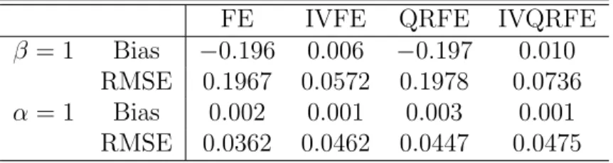
Table 1: Location Shift Model: Bias and RMSE of estimators for normal distribution (T = 10 and N = 100)
FE IVFE QRFE IVQRFE
β = 1 Bias −0.196 0.006 −0.197 0.010
RMSE 0.1967 0.0572 0.1978 0.0736
α= 1 Bias 0.002 0.001 0.003 0.001
RMSE 0.0362 0.0462 0.0447 0.0475
Table 2: Location Shift Model: Bias and RMSE of estimators for t3 distribution (T = 10
and N = 100)
FE IVFE QRFE IVQRFE
β = 1 Bias −0.201 −0.004 −0.159 0.009
RMSE 0.2075 0.0619 0.1531 0.0542
α= 1 Bias 0.001 0.001 −0.001 −0.001
RMSE 0.0396 0.0471 0.0342 0.0363
the bias in the mismeasured variable coefficient of the FE and QRFE estimators are severe. However the coefficients for the IVFE and IVQRFE are approximately unbiased. Moreover, since we do not consider any correlation among the regressors, as expected, the coefficient of the perfectly measured variable is approximately unbiased in all cases.
Table 1 shows that when the disturbances are sampled from a normal distribution, as expected, the mismeasured regressor coefficient is downward biased for the FE case, but the IVFE is approximately unbiased. Similarly, in the presence of errors in variables, the QRFE estimator proposed by Koenker (2004) is downward biased and IVQRFE is able to reduce the bias. In summary, estimates are biased in both the FE and the QRFE cases, and the IV strategy is able to considerably diminish the bias for both LS and QR cases. Regarding the RMSE, in the Gaussian condition, the LS based estimators perform better than the respective QR estimators. Thus, under Gaussian conditions, the IVQRFE is capable to reduce the bias but it has a larger RMSE when compared with the IVFE.
Table 2 presents simulations for the t3-distribution case. The β estimates of FE and
QRFE are biased, and the FE has a larger bias when compared with the same estimator in the Gaussian case. The IVQRFE is approximately an unbiased estimator for both coefficients. Interestingly, in the non-Gaussian heavy-tailed condition, the RMSE of IVQRFE is smaller than the RMSE of IVFE, evidencing that there are gains in efficiency by using a robust estimator.
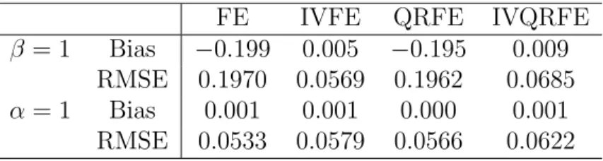
Table 3: Location-Scale Shift Model: Bias and RMSE of estimators for normal distribution (T = 10 and N = 100)
FE IVFE QRFE IVQRFE
β = 1 Bias −0.199 0.005 −0.195 0.009
RMSE 0.1970 0.0569 0.1962 0.0685
α= 1 Bias 0.001 0.001 0.000 0.001
RMSE 0.0533 0.0579 0.0566 0.0622
Table 4: Location-Scale Shift Model: Bias and RMSE of estimators for t3 distribution
(T = 10 and N = 100)
FE IVFE QRFE IVQRFE
β = 1 Bias −0.208 0.004 −0.146 0.007
RMSE 0.2086 0.0779 0.1475 0.0480
α= 1 Bias 0.002 0.003 0.004 0.001
RMSE 0.2797 0.2801 0.0791 0.0789
Tables 3 and 4 present bias and RMSE results for the location-scale-shift model for the normal and t3 distributions respectively. In both cases the FE and QRFE estimators are
downward biased and the IVFE and IVQRFE are approximately unbiased. Note that the IVQRFE estimator presents a considerable smaller bias than QRFE and much more precision when compared with IVFE in the t3 case.
4
Empirical application:
Investment, Tobin’s
q
and
cash flow
As pointed out in Wansbeek (2001), the most frequent application of measurement error techniques is in the estimation of investment models using Tobin’s q. This variable is the ratio of the market valuation of a firm and the replacement value of its assets. Firms with a high value of q are considered attractive as to the investment opportunities, whereas a low value of q indicates the opposite. Since the operationalization of q is not clear-cut and unambiguous, estimation poses a measurement error problem. Many empirical investment studies found a very disappointing performance of the q theory of investment, although this theory has a good performance when measurement error is purged as in Erickson and Whited (2000). In parallel, investment theory is also interested in the effect of cash flow, as the theory predicts that financially constrained firms are more likely to rely on internal funds
to finance investment (see for instance Alti, 2003; Almeida, Campello and Weisbach, 2004). However, Erickson and Whited (2000) argue that cash flow has no effect on investment once measurement error in Tobin’sq is taken into account.
There are distinct advantages in exploiting panel data on individual firms (see for in-stance Blundell, Bond, Devereux and Schiantarelli, 1992). In the first place it allows testing the theory, developed in the context of a ‘representative’ firm, in the context of many firms, so reducing econometric problems introduced by aggregation across firms. Aggregation prob-lems may be important here since the standard q model is specified in ratios and there are clear nonlinearities. Secondly, the estimates are obtained by using both the time-series and cross-sectional variation in the data. This contributes to their precision and also allows con-sistent estimation in the presence of firm specific effects correlated both with investment and
q values. Although not reported, pooled and FE estimates differ in our estimation, which determines that firm individual FE need to be controlled for in our model.
We argue that QR is useful to describe differences in investment ratios across firms in the presence of unobserved heterogeneity. Unobserved characteristics (for the econometri-cian) across firms may be due to several reasons. The ability of managers (insiders) or the characteristics of investors (outsiders) can be named as the main unobservable component. For instance, Bertrand and Schoar (2003) find that a significant extent of the heterogeneity in investment, financial, and organizational practices of firms can be explained by managers ’style’. Walentin and Lorenzoni (2007) develop a model of financially constrained firms fi-nanced partly by insiders, who control its assets, and partly by outside investors. When their wealth is scarce, insiders earn a rate of return higher than the market rate of return, that is, they receive a quasi-rent on invested capital. Therefore, differences in insiders and outsiders characteristics across firms may contribute to differences in investment behavior. Additional heterogeneity may be due to differences in firms’ capital structure. Chirinko (1993) shows that when the q theory is expanded for the possibility that the value of the firm depends on two or more capital inputs with differing adjustment cost technologies, the econometric equation following from optimizing behavior includes q as well as additional variables (e.g. inventory, research and development). In the upper conditional quantiles of investment, investment may be driven by insiders knowledge of business opportunities or a particular capital structure that requires more investment, and therefore, we expect that investment would be more responsive to changes in q and cash flow, as the firms would use all available resources to finance its projects. Moreover, high investment ratios reduce the
marginal productivity of additional investment, and therefore, it would be difficult to get additional resources. In other words,qand cash flow sensitivities will be higher in the upper quantiles of investment than in the lower quantiles.
In contrast with the interpretation of QR in cross-section, by controlling for the firm-specific characteristics, the quantiles should be interpreted in terms of the pairs firm-year. In this case, low (high) quantiles refer to firms in periods with unusually low (high) investment ratios when conditioning on other time-variant observable information. This determines that the same firm can be at different quantiles in different periods, which is in line with the idea that firm’s behavior will change depending on their investment needs.
The baseline model in the literature is
Iit/Kit =ηi+βqit∗ +αCFit/Kit+uit, (26)
where I denotes investment, K capital stock, CF cash flow, q∗ well-measured Tobin’s q,
η is the firm-specific effects and u is the innovation term. Our objective is estimating the following conditional quantile function:
QI/K(τ|η, CF/K, q) = ηi(τ) +β(τ)qit∗ +α(τ)CFit/Kit. (27)
As mentioned earlier, if q is subject to measurement error, estimates of β(τ) will be biased down (assumingβ(·)>0), but this problem can be ameliorated by using instrumental variables.
We follow Almeida, Campello, and Weisbach (2004) approach by considering a sample of manufacturing firms (SICs 2000 to 3999) over the 1980 to 2005 period with data available from COMPUSTAT’s P/S/T, Full Coverage. Only firms with observations in every year are used, in order to construct a balanced panel of firms for the 26 year period.13 Moreover,
following those authors we eliminate firms for which cash-holdings exceeded the value of total assets and those displaying asset or sales growth exceeding 100%. Our final sample consists of 4550 firm-years and 175 firms. Summary statistics of the variables employed in our econometric specifications appear in Table 5. Because we only consider firms that report information in each of the 26 years, the sample consists mainly of relatively large firms. Although this reduces the sample heterogeneity in terms of credit constraints (e.g.
presumably firms with market information for continuous 26 years are credit unconstrained), it serves for our purposes of studying firm heterogeneity along different quantiles.
Table 5: Summary statistics
Variable Mean Std.Dev. 0.25 quantile Median 0.75 quantile
I/K 0.203 0.145 0.119 0.174 0.249 q 0.778 0.265 0.617 0.738 0.873 CF/K 0.414 0.444 0.211 0.345 0.534 ∆I/K -0.003 0.168 -0.050 -0.000 0.045 ∆q -0.004 0.136 -0.057 -0.004 0.049 ∆CF/K -0.000 0.302 -0.066 0.006 0.074
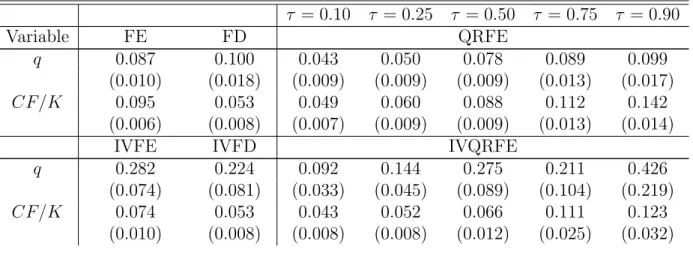
Table 6 report the regression estimates. The first column reports least squares within group (FE) estimators without (first set of rows) and with instruments (last set of rows, IVFE). The second column reports least squares in first differences for the same set of rows (FD and IVFD respectively). Following Biorn (2000) we use lags of the first differences of the mismeasured variable as instruments for fixed effects, and lags in levels for the first differences estimator. The last five columns report QR estimates with fixed effects (QRFE). Our proposed estimator, IVQRFE, appears in the last rows where the same instruments used in FE are employed. IV estimates are reported with one instrument (∆qt−1 for the model in
levels,qt−2 for FD) and with two instruments (∆qt−1,∆qt−2 for the model in levels,qt−2, qt−3
for FD) to assess the sensitivity of the estimates to the instrument selection.14
Table 6: Econometric results
τ = 0.10 τ = 0.25 τ = 0.50 τ = 0.75 τ = 0.90 Variable FE FD QRFE q 0.087 0.100 0.043 0.050 0.078 0.089 0.099 (0.010) (0.018) (0.009) (0.009) (0.009) (0.013) (0.017) CF/K 0.095 0.053 0.049 0.060 0.088 0.112 0.142 (0.006) (0.008) (0.007) (0.009) (0.009) (0.013) (0.014)
IVFE IVFD IVQRFE
q 0.282 0.224 0.092 0.144 0.275 0.211 0.426 (0.074) (0.081) (0.033) (0.045) (0.089) (0.104) (0.219)
CF/K 0.074 0.053 0.043 0.052 0.066 0.111 0.123 (0.010) (0.008) (0.008) (0.008) (0.012) (0.025) (0.032) 14Although not reported, we also use least squares projections as a different set of instruments in the QR
estimations. We consider the projection ofqit on each respective instrument and the exogenous variables, i.e. the fixed effects and cash flow. In every case, we obtain similar results.
Inst. ∆qt−1 qt−2 ∆qt−1 q 0.203 0.181 0.086 0.116 0.245 0.223 0.322 (0.051) (0.080) (0.022) (0.033) (0.057) (0.082) (0.167) CF/K 0.083 0.053 0.044 0.056 0.067 0.109 0.132 (0.008) (0.008) (0.029) (0.029) (0.046) (0.061) (0.078) Inst. ∆qt−1,∆qt−2 qt−2, qt−3 ∆qt−1,∆qt−2
Notes: Standard errors in parenthesis. Sample of 4550 firm-years and 175 firms. FE: fixed effects least squares; FD: first differences least squares; QRFE: quantile regression with fixed effects; IVFE: instrumental variables fixed effects least squares; IVFD: instrumental variables fixed differences least squares; IVQRFE: instrumental variables quantile regression fixed effects.
Both FE and FD estimators give similar results for the effect of Tobin’s qon investment, implying that firms with higher q values would invest more. In particular, the q-sensitivity of investment is close to 0.10. Cash flow appear as positive and statistically significant. However, the FD estimate of cash flow is half of that in FE. When instrumental variables are used, the effect of Tobin’s q raises considerably, which is in line with the presence of measurement error in this variable. By contrasting the effect of the instrumental variables across different estimates, it can be concluded that measurement error in Tobin’s q reduces its effect by a half. Moreover, the point estimates of cash flow do not change, which can be interpreted as the fact that measurement error in Tobin’s q has no spillover measurement error to cash flow. In turn, this contradicts Erickson and Whited (2000) statement that cash flow “does not matter” as it has a highly significant (mean) effect.
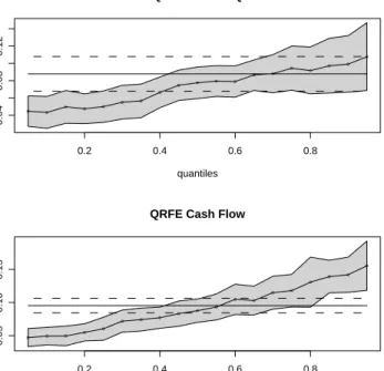
FE, FD and QRFE point estimates differ both in terms of Tobin’sqand cash flow effects. QRFE estimates are monotonically increasing in τ, ranging from 0.045 for τ = 0.05 to 0.11 at τ = 0.95 (see figure 1). In terms of the Tobin’s q point estimates, QRFE is below FE
for τ < 0.75 and below FD almost everywhere. As a result, firms-years with unusually
high investment ratios will be very responsive to changes in their market valuation. In a similar token, the effect of cash flow on investment is monotonically increasing in τ. This determines that firms with conditionally high investment ratios have a higher propensity to use additional internal resources to finance investment than those with low investment ratios.
The use of IVQRFE differ from QRFE point estimates in a similar way as IVFE and IVFD differ from FE and FD respectively (see figures 2 and 3). However, in this case, the monotonicity is weakened in the q-sensitivity of investment. For low quantiles, QRFE and IVQRFE provide similar point estimates. However, both estimators differ greatly as τ in-creases. This suggests an interesting asymmetry in terms of the measurement error problem,
as it may manifest itself mostly for firms-years in the upper quantiles of the investment distribution. Point estimates for IVQRFE are particularly high for τ ≥ 0.90, reaching a
q-sensitivity of 0.4. Nevertheless, IVQRFE has bigger standard errors than both IVFE and QRFE. In fact for τ >0.25 the IVFE confidence interval is contained in the IVQRFE inter-val, while QRFE interval is always contained. In addition, QRFE and IVQRFE give similar estimates in terms of the cash flow sensitivity of investment, which reassures the fact that the effect of this variable on investment is not due to measurement error in Tobin’s q and that its effect is increasing inτ. Finally, it can be observed that the effect of expanding the instruments’ set on the IVQRFE point estimates is in line with that in least squares model. That is, using only ∆qt−1 produces a higher estimate for theq-sensitivity of investment than
Figure 1: FE and QRFE 0.2 0.4 0.6 0.8 0.04 0.08 0.12 quantiles coefficient QRFE Tobin's Q o o o o o o o o o o o o o o o o o o o 0.2 0.4 0.6 0.8 0.05 0.10 0.15 quantiles coefficient
QRFE Cash Flow
o o o o o o o o o o o o o o o o o o o
Figure 2: IVFE and IVQRFE (Instrument ∆qt−1) 0.2 0.4 0.6 0.8 0.0 0 .2 0.4 0 .6 0.8 quantiles coefficient IVQRFE Tobin's Q o o o o o o o o o o o o o o o o o o o 0.2 0.4 0.6 0.8 0.05 0.15 quantiles coefficient
IVQRFE Cash Flow
o o o o o o o o o o o o o o o o o o o
Figure 3: IVFE and IVQRFE (Instruments ∆qt−1,∆qt−2) 0.2 0.4 0.6 0.8 0.0 0 .2 0.4 0 .6 quantiles coefficient IVQRFE (DL1x DL2x) Tobin's Q o o o o o o o o o o o o o o o o o o o 0.2 0.4 0.6 0.8 -0.05 0 .05 0 .15 0 .25 quantiles coefficient
IVQRFE (DL1x DL2x) Cash Flow
o o o o o o o o o o o o o o
o
o o o o
5
Conclusion
We propose the use of an instrumental variables strategy for estimation and inference in quantile regression FE panel data models with measurement errors. Quantile regression methods allow one to explore a range of conditional quantiles exposing a variety of forms of conditional heterogeneity under less compelling distributional assumptions and provide a framework for robust estimation and inference. Most instrumental variables estimators are at least partly based on the intuition that first differencing yields a model free of FE. Despite its appeal as a procedure that avoids the estimation of the individual effects, differencing transformation to eliminate the FE is not available in the quantile regression framework, and we are required to deal directly with the full problem. We derive an approximation to the bias in the QRFE estimator in the presence of a mismeasured variable. We suggest the use of an instrumental variables strategy for estimation based on Chernozhukov and Hansen (2006, 2008) that reduces the bias in the resulting point estimates. We show that the IV FE panel estimator is consistent and asymptotically normal, provided that both N
and T grow to infinity and Na/T → 0, for some a > 0. In addition, we suggest Wald and Kolmogorov-Smirnov type of tests for general linear hypotheses, and derive the respective limiting distributions.
Monte Carlo studies are conducted to evaluate the finite sample properties of the quan-tile regression instrumental variables estimator for different types of distributions. It is shown that the estimator proposed by Koenker (2004) is severely biased in the presence of mismeasured variables, while the IVQRFE sharply reduces the bias in this environment. In addition, IVQRFE has a better performancevis-a-vis the IV least squares based approach in terms of the bias and root mean square error of the estimators for non-Gaussian heavy-tailed distributions.
Finally, we apply the instrumental variables estimator to the most frequent application of measurement error techniques, the Tobin’s q theory of investment in corporate finance. We show that the IVQRFE estimator purges for measurement error in a similar way to standard IV techniques in the least squares framework, but it shows interesting asymmetries in terms of the measurement error correction across quantiles.
Appendix 0:
η
’s with Pure Location Shift
The η’s are intend to capture some individual specific source of variability, or “unobserved heterogeneity,” that was not adequately controlled for by other covariates. In most applica-tions the time series dimension T is relatively small compared to the number of individuals
N. Therefore, it might be difficult to estimate aτ-dependent distributional individual effect. In this case, we still can estimate an individual specific location-shift effect.
Consider the following model for conditional quantile functions
Qyit(τ|x ∗ it, zit) =ηi+x∗0itβ(τ) +z 0 itα(τ), (28) where xit=x∗it+it.
In this formulation the η’s have a pure location shift effect on the conditional quantiles of the response variable. The effects of the covariates (xit, zit) are allowed to depend upon
the quantile, τ, of interest but the η’s do not. From the availability of a valid instrument,
w, following Koenker (2004) and Chernozhukov and Hansen (2006, 2008) to estimate model (28) for several quantiles simultaneously we propose the following estimator
ˆ β(τk) = argmin β kˆγ(β, τk)k, (29) where (ˆη(β),αˆ(β, τ),γˆ(β, τ)) = argmin η,α,γ K X k=1 N X i=1 T X t=1 υkρτ(yit−d0itη−x 0 itβ(τk)−z0itα(τk)−w0itγ(τk)), (30) and υk are the weights that control the relative influence of the K quantiles {τ1, ..., τK} on
the estimation of the ηi parameter. The design matrix for the problem of estimating K >1
is as follows:
[υ ⊗(In⊗1T)...Υ⊗X...Υ⊗Z...Υ⊗W],
where In is a N ×N identity matrix, 1T is a T ×1 vector of ones, Υ is a K ×K diagonal
matrix with the weightsυ in the diagonal. Moreover, as Koenker (2004) observes, in typical applications the above design matrix of the full problem is very sparse, i.e. has mostly zero elements. Standard sparse matrix storage schemes only require space for the non-zero elements and their indexing locations, and this considerably reduces the computational effort and memory requirements in large problems.
The optimization may become very large depending on the number of estimated quantiles. Therefore, instead of using a grid search we use a numerical optimization function in R
(optim). As starting values, we use the parameters of “naive” estimation (28) without any instruments. It is important to notice that all the results presented previously are still valid. In addition, inference is essentially the same to that presented in section 2. However, the elements of the variance-covariance matrix in Theorem 2 should now be as in the design matrix presented above.
Appendix 1: Analogy between QRIV and 2SLS
Regular OLS Case
Consider the following model
y=X0β+Z0α+u
where X is the endogenous variable, Z is the exogenous covariate and u is the error term. LetW be a valid instrument for X. In the two stage least squares procedure
ˆ β = (X0PMZWX) −1 X0PMZWy, (31) where PMZW = MZW(W 0M
ZW)−1W0MZ. Note that if the same number of columns in X
is the same as in W, then W0MZX is an invertible matrix and we can simplify the above
equation to
ˆ
β = (W0MZX)−1W0MZy. (32)
Grid Case
Now we consider the Grid case. Define a grid for β, {βj, j = 1, ..., J}, and for given βj ,
consider the following regression
y−X0βj =Z0α+ ˆW0γ+v,
where ˆW is an instrument for X, defined as the projection ofX onZ and W, ˆ
W := ˆX =Z0λˆ+W0δ.ˆ
The estimator ˆγ(βj) is
ˆ
Now define the estimator of ˆβ as ˆ
β = arg min
β kγˆ(β)kA,
where kˆγ(β)kA = ˆγ(β)0Aγˆ(β), ˆγ(β) is the vector containing the estimates ˆγ(βj), and A is
the identity matrix. Noticing that MZWˆ =MZW(W0MZW)−1W0MZX, and from the first
order condition ˆ
β = (X0MZW(W0MZW)−1W0MZX)−1X0MZW(W0MZW)−1W0MZy.
Using the definition of PMZW we have ˆ
β = (X0PMZWX) −1
X0PMZWy, (33)
which is the same estimator as in equation (31). When the model is exactly identified ˆ
β = (W0MZX)−1W0MZy, (34)
which is the same estimator as in equation (32).
Appendix 2: Proof of the Theorems
The next three Lemmas help in the derivation of the results. The first Lemma shows the identification of the parameters. The second guarantees a law of large numbers. The third Lemma states anArgmax Process argument which is helpful in the derivation of consistency. Later we show consistency of ˆθ(τ).
Lemma 2 Given assumptions A1-A6, (η(τ), β(τ), α(τ)) uniquely solves the equations
E[ψ(Y −Dη−Xβ−Zα) ˇX(τ)] = 0 overE ×B×A.
Proof. We want to show that (η(τ), β(τ), α(τ)) uniquely solves the limit problem for eachτ, that isη(β∗(τ), τ) = η(τ),β∗(τ) = β(τ), andα(β∗(τ), τ) =α(τ). Letψ(u) := (τ−I(u <0)). Define: Π(η, β, α, τ) :=E[ψ(Y −D0η(τ)−X0β(τ)−Z0α(τ)) ˇX(τ)] H(η, β, α, τ) := ∂ ∂(η, β, α)E[ψ(Y −D 0 η(τ)−X0β(τ)−Z0α(τ)) ˇX(τ)]
By assumption A2 H(η, β, α, τ) is continuous in (η, β, α) and full rank, uniformly over
(η, β, α) → Π(η, β, α, τ) is assumed the be simply connected. As in Chernozhukov and Hansen (2005), the application of Hadamard’s global univalence theorem for general met-ric spaces, e.g. Theorem 1.8 in Ambrosetti and Prodi (1995), yields that the mapping Π(·,·, τ) is a homeomorphism (one-to-one) between (E ×B ×A) and Π(E,B,A, τ), the image ofE ×B×A under Π(·,·, τ). Since (η, β, α) = (η(τ), β(τ), α(τ)) solves the equation Π(η, β, α, τ) = 0; and thus it is the only solution in (E ×B×A). This argument applies for every τ ∈ T . So, we have that the true parameters (η, β, α) = (η(τ), β(τ), α(τ)) uniquely solve the equation
E[ψ(Y −D0η−X0β−Z0α−W00) ˇX(τ)] = 0. (35) Define φ := (η, α, γ). By assumption and in view of the global convexity of Q(β, φ, τ) in φ
for each τ and β, φ(β, τ) is defined by the subgradient condition
E[ψ(Y −D0η(β, τ)−X0β−Z0α(β, τ)−W0γ(β, τ)) ˇX(τ)]v ≥0 (36) for all v :φ(β, τ) +v ∈E ×A ×G.
In fact, if φ(β, τ) is in the interior of E ×A ×G, it uniquely solves the first order condition version of (36)
E[ψ(Y −D0η(β, τ)−X0β−Z0α(β, τ)−W0γ(β, τ)) ˇX(τ)] = 0. (37) We need to find β∗(τ) by minimizing kγ(β, τ)k over β subject to (36) holding. By (35)
β∗(τ) = β(τ) makes kγ(β∗, τ)k = 0 and satisfies (37) and hence (36) at the same time. According to the preceding argument, it is the only such solution. Thus, also by (37) (η(β∗(τ), τ) =η(τ), α(β∗(τ), τ) = α(τ)). Lemma 3 Letξit(τ) = d0itη(τ) +x 0 itβ(τ) +z 0 itα(τ) +w 0 itγ(τ) anduit(τ) = yit−ξit(τ). Letϑ := (η, β, α, γ)
be a parameter vector in V :=E ×B×A ×G. Let
δ= δη δβ δα δγ = √ T(η−η(τ)) √ N T(β−β(τ)) √ N T(α−α(τ)) √ N T(γ−γ(τ)), .
Under conditions A1-A6, sup ϑ∈V (N T)−1 X i X t h ρτ(uit(τ)− d0itδη √ T − x0itδβ √ N T − z0itδα √ N T − wit0 δγ √ N T)−ρτ(uit(τ)) (38) −E[ρτ(uit(τ)− d0itδη √ T − x0itδβ √ N T − z0itδα √ N T − wit0 δγ √ N T)−ρτ(uit(τ))] i =op(1).