2017 IEEE INTERNATIONAL WORKSHOP ON MACHINE LEARNING FOR SIGNAL PROCESSING, SEPT. 25–28, 2017, TOKYO, JAPAN
LEARNING EMBEDDINGS FOR SPEAKER CLUSTERING BASED ON VOICE EQUALITY
Yanick X. Lukic, Carlo Vogt, Oliver D¨urr, and Thilo Stadelmann
Zurich University of Applied Sciences, Winterthur, Switzerland
ABSTRACT
Recent work has shown that convolutional neural networks (CNNs) trained in a supervised fashion for speaker identifica-tion are able to extract features from spectrograms which can be used for speaker clustering. These features are represented by the activations of a certain hidden layer and are called em-beddings. However, previous approaches require plenty of additional speaker data to learn the embedding, and although the clustering results are then on par with more traditional ap-proaches using MFCC features etc., room for improvements stems from the fact that these embeddings are trained with a surrogate task that is rather far away from segregating un-known voices - namely, identifying few specific speakers.
We address both problems by training a CNN to extract embeddings that are similar for equal speakers (regardless of their specific identity) using weakly labeled data. We demon-strate our approach on the well-known TIMIT dataset that has often been used for speaker clustering experiments in the past. We exceed the clustering performance of all previous approaches, but require just 100 instead of 590 unrelated speakers to learn an embedding suited for clustering.
Index Terms— Speaker Clustering, Speaker Recogni-tion, Convolutional Neural Network, Speaker Embedding
1. INTRODUCTION
Speaker clustering handles the”who spoke when”challenge in a given audio recording without knowing how many and which speakers are present in the audio signal. It is called speaker diarization when the task of segmenting the audio stream into speaker-specific segments is handled simulta-neously [1]. The problem of speaker clustering is eminent in digitizing audio archives like e.g. recordings of lectures, conferences or debates [2]. For their quantitative indexing, automatic extraction of key figures like number of speakers or talk time per person is important. This further facili-tates automatic transcripts using existing speech recognition procedures, based on the accurate automatic assignment of speech utterances to groups that each represent a (previously unknown) speaker.
The lack of knowledge of the number and identity of speakers leads to a much more complex problem compared to
the related tasks of speaker verification and speaker identifi-cation, and in turn to less accurate results. One reason is that well-known speech features and models, originally fitted to the latter tasks, might not be adequate for the more complex clustering task [3]. The use of deep learning methods offers a solution [4]: in contrast to classical approaches (e.g., based on MFCC features and GMM models [5]), where general fea-tures and models are designed manually and independently for a wide variety of tasks, deep models learn hierarchies of suitable representations for the specific task at hand [6]. Espe-cially convolutional neural networks (CNNs) have proven to be very useful for pattern recognition tasks mainly on images [7], but also on sounds [8]. Previous work [9] has shown that CNNs are able to learn a voice-specific vector representation (embedding) suitable for clustering when trained for the sur-rogate task of speaker identification. The authors report state of the art results for speaker clustering using an embedding learned from590different speakers.
In this paper, we investigate a novel training approach for CNNs for speaker clustering that learns embeddings more di-rectly based on pairwise voice equality information of speech snippets (i.e., the binary information if the two snippets come from the same speaker or not). This weak labeling is neither a fitting to particular individuals, nor depending on hard to obtain voice similarity measures (i.e., real-valued distances amongst snippets). For evaluation, we focus on the pure speaker clustering performance, given its role as a perfor-mance bottleneck in the complete diarization process [3]. Section 2 reviews related work and introduces our approach. Section 3 reports on our results that not only reach state of the art consistently with one approach and improve the clustering quality in certain scenarios, but also reduce the necessary amount of pre-training data to 17%. We also report on a number of experiments in order to give insight on which part of our system is responsible for the improved results. We conclude the paper with an outlook in section 4.
2. LEARNING SPEAKER DISSIMILARITY 2.1. Related work
The design of CNNs makes it possible to recognize patterns in minimally preprocessed digital images or other data with
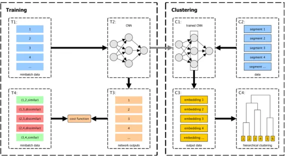
Fig. 1. Our overall speaker clustering process. Shown are the training steps (T1–T4) and the steps for the generation of speaker representations which are then hierarchically clustered (C1–C4).
two dimensional structure by exploiting local connectivity. CNNs and other deep neural network (DNN) architectures thus have become the standard technique in many percep-tual tasks [10][11][12][13]. Notable examples on audio data include Lee et al., who demonstrate how spectrograms can serve as inputs for a deep architecture in various audio recog-nition tasks [4]; and van den Oord and colleagues who build a generative model for sound (speech and otherwise) using a CNN variant [14]. Salamon et al. show how data augmenta-tion serves to use CNNs for environmental sound classifica-tion, having only scarce data [15]. Milner and Hain attempt speaker diarization by iteratively re-labeling an initial set of utterances using DNNs per utterance that have been adapted from a single speaker recognition DNN, and then re-training the DNNs per resulting segment [16]. McLaren et al. address speaker recognition by using senone probabilities computed by a CNN, reaching results on par with an i-vector approach [17], and Sell et al. use a similar approach for speaker di-arization [18]. However, previous work in the field of learning speaker characteristics using neural networks mostly relies on preprocessed features like MFCCs and doesn’t use the feature learning capabilities of CNNs [19][20].
Recent advances have shown that it is possible to learn speaker-specific features from hidden layers of neural net-works. Yella, Stolcke and Slaney used speaker-specific fea-tures derived from a 3 layer neural network together with MFCCs to subsequently feed them into a GMM/HMM system for speaker clustering [20]. This concept ofspeaker embed-dingswas further developed by Rouvier et al. through speaker representations derived from a non-convolutional neural net-work, using a super-vector obtained from a GMM-UBM as input vector [21].
It has been shown in [9] that CNNs are able to learn valu-able features from spectrograms for speaker clustering. The authors use a single fully connected layer of a trained classi-fication network to extract speaker embeddings (feature vec-tors) and subsequently cluster unknown speakers, achieving state of the art results. In contrast to this approach, we change the learning process fundamentally in this paper by using pair-wise constraints instead of relying on a rather unrelated surro-gate task for the creation of the speaker embeddings. This ap-proach has been introduced in [22] using the MNIST dataset and was further developed in [23] to automatically discover image categories in unlabeled data. The process is similar in spirit to a siamese architecture [24], but building all possible pairs of snippets per mini-batch here allows for much more efficient training.
2.2. Our approach
Our approach consists of two major stages (see Fig. 1): train-ing (T1–T4) and clustertrain-ing (C1–C4). The traintrain-ing stage is based on the work of Hsu and Kira [22]. Training is per-formed using mini-batch gradient descent, whereas the spec-trograms are built exactly as in [9]. To attain a high diversifi-cation of the mini-batch composition (T1), for each member a random sentence from the training set is selected, and from this a random snippet of one second is used. A snippet has dimensionality128×100(f requency×time). We com-bine100 such snippets in a mini-batch and let the network (T2) compute an output (T3) for each snippet in the mini-batch. An output consists of the activations of a dense layer. Then, all possible pairs of these outputs are built, accompa-nied by weak labels stating whether the two original snippets
Fig. 2. The shown architecture is used for all experiments. In the convolutional layers,F×T corresponds to the dimension of the appliedf requency×timefilters.
are equal (same speaker) or not (different speakers) (T4). The error per pair is calculated by a cost function associated with the Kullback-Leibler divergence (KL divergence) to minimize the distance between equal pairs while maximizing the dis-tance for unequal pairs [22]. This trains embeddings focused on voice equality and, by implication, similarity.
For a given pair of snippetsxp andxq, imagine that the networkf produces the embeddingsP andQof dimension-alityk, respectively. These can be regarded as two discrete probability distributionsP = f(xp)andQ = f(xq)over high-level voice-related features, for which the KL divergence is defined as follows: KL(PkQ) = k X i=0 Pilog( Pi Qi ) (1)
To use the KL divergence in the cost function, two indi-cator functionsIs andIds are introduced, whereIs = 1if
(xp, xq)is an equal pair w.r.t. voice, andIds= 1if it is a dis-similar pair, otherwise0. The hyperparametermarginin the hinge-loss part of the cost function sets the maximum margin between dissimilar pairs; we set it to2as proposed in [22].
cost(PkQ) =Is(xp, xq)·KL(PkQ)
+Ids(xp, xq)·max(0,margin−KL(PkQ)) (2) The total costL for the pair(xp, xq)is calculated sym-metrically via:
L(P,Q) = cost(PkQ) + cost(QkP) (3) In the clustering stage, the trained network (C1) is then used to generate embeddings from given speech utterances of unknown speakers (segments in C2). Utterances are split into non-overlapping1s long snippets, then an embedding (C3) is extracted per snippet from one of the hidden layers (specified below) by using the activations of this layer. An embedding per utterance is formed by averaging over all embeddings of its snippets. Finally, as in [9], agglomerative hierarchical clustering (C4) withcomplete linkageis performed using the
cosinedistances between these mean embeddings of each ut-terance. We use the misclassification rate (MR) as defined by
Kotti et al. [25] to evaluate the clustering performance in a way comparable to related work: AMRof0confirms perfect assignment (all utterances of the same speaker in one cluster) and aMRof1means that all utterances are assigned wrongly (falsely separated or mixed up in non-pure clusters). TheMR is defined as follows: M R= 1 N Nc X j=1 ej. (4)
N corresponds to the total number of utterances to be clustered, Nc to the number of speakers (=clusters) and ej to the number of incorrectly assigned utterances of speakerj. The reportedMRfor an experiment corresponds to the lowest MRreached by varying the cutting point of the agglomerative hierarchical clustering manually (we thus ignore the problem of optimal cut point detection to focus on the task of cluster-ing in an optimal order in accordance with [3]). The reported confidence intervals are calculated using Wilson method for a binomial probabilities with2·N observations andM R·N
successes.
Note that the proposed clustering method is not learned completely end-to-end. However, the surrogate task (learn-ing to produce similar distributions for speech snippet pairs from the same speaker, based on short utterances) of the CNN is much closer to the final clustering task as compared to when training a standard speaker identification model to ex-tract speaker embeddings (where the surrogate task is to clas-sify specific voices, thus focusing on the characteristics of the concrete speakersx1..xNc). The learned embeddings
there-fore should be more suitable for clustering.
The architecture of our CNN is derived from [9] (com-pare Fig. 1, T2 and C1). We enhance it by using batch norm layers [26] after each convolutional layer and the first dense layer, and by changing the cost function as described above. Apart from that, the architecture stays the same. The detailed modified architecture is shown in Fig. 2.
3. EXPERIMENTAL SETUP AND RESULTS
All experiments are carried out on the TIMIT dataset using the exact experimental setup as in previous work to be com-parable [9][3]. Especially data splits and the used subsets of speakers for training and clustering follow these provisions closely. This means that when we perform clustering ofNc speakers, we have overall2·Ncutterances in our data set: two per speaker, where one is composed of the first8sentences of the speaker (lexicographically ordered by filename), and the other from the remaining two sentences, yielding an average utterance lengths of20and5seconds, respectively.
We carry out two major experiments: First, we test in a minimal setup whether it is possible to learn the distances (w.r.t. voice equality) between spectrograms. Second, we evaluate clustering performance on up toNc = 80speakers, using our network pretrained onNt= 100unrelated training speakers.
3.1. Feasibility of KL divergence-related cost
To assess whether our approach is able to learn the KL divergence-related cost function for two snippets, we train a network withNt = 10speakers and then clusterNc = 5 andNc = 10 unrelated speakers on the activations of all layers separately. Thereby we can ascertain that the network is able to learn from the given constraints. Additionally, we can observe whether this cost formulation provides an advan-tage for speaker embedding extraction for clustering over the approach in [9]. We thus replicate as much of the training procedure from there (except the cost function) as possible, including training by stochastic gradient descent (SGD) with Nesterov momentum.
Performing the clustering experiment usingNc = 5 un-known speakers we achieve aMRof0.0on all layers. How-ever, when looking at the t-SNE [27] (with cosine metric) plot per snippet in Fig. 3, we observe that the first dense layer L7 provides a much better visual clustering than the third dense layer L11. This is substantiated when performing the cluster-ing experiment withNc = 10unknown speakers: clustering on the third dense layer performs worse (MR of 0.3) than on the activations of both other dense layers, where aMRof
0.1is achieved. Thus, our speaker embeddings using the new similarity-based training regime clearly work, and seem to do so better if we extract them from lower dense layers.
3.2. Improved optimization to cluster more speakers
When increasing the complexity of the experiment by naively training a bigger network (Nt = 100speakers) and cluster-ing more speakers (Nc = 40speakers), the clustering per-formance decreases significantly (MR = 0.375). Hence, we try different additional optimization approaches using Adam [28], Adadelta [29] and, for reasons of comparability, also SGD without any momentum. We choose the algorithms’
Fig. 3. Clustering quality visualization using t-SNE plots for embeddings extracted from the third dense layer L11 (left) and the first dense layer L7 (right). Different colors corre-spond to different speakers.
hyperparameters based on preceding experiments as follows: SGD with learning rate 0.001; Nesterov with learning rate
0.001 and momentum 0.9; Adam with learning rate 0.001,
β1 = 0.9,β2 = 0.999and = 10−8; Adadelta with learn-ing rate1.0,ρ= 0.95and= 10−6. All resulting networks are trained for100000−300000mini-batches (with mini-batch sizeB = 100). The results for the clustering set ofNc = 40 speakers are shown in Tab. 1.
SGD results in highMRvalues, while Nesterov momen-tum performs better. More complex optimizers like Adam and Adadelta reach even better results. Additionally, they still show an upward trend after10K mini-batches. There-fore, we train these for additional mini-batches including all validation data. While Adam starts to show a performance decrease, Adadelta still improves for additional 10K mini-batches before leveling off on the best performing dense layer (L7).
3.3. Embeddings of lower layers for better generalization
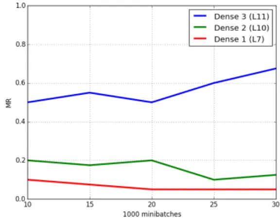
Fig. 4. AchievedMRsfor the different training stages (num-bers of mini batches) of the Adadelta-trained network.
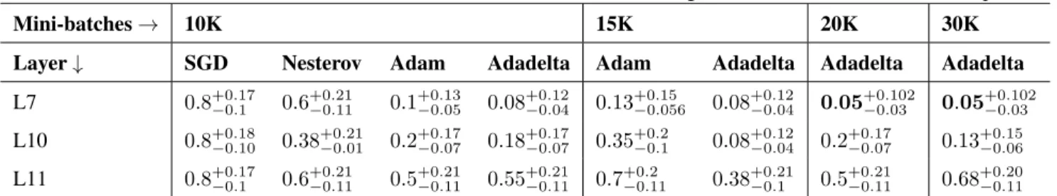
Table 1. Estimates and 0.95 Wilson-Confidence intervalls ofMRs for all training methods forNc= 40unknown speakers
Mini-batches→ 10K 15K 20K 30K
Layer↓ SGD Nesterov Adam Adadelta Adam Adadelta Adadelta Adadelta
L7 0.8+0.17−0.1 0.6+0.21−0.11 0.1+0.13−0.05 0.08+0.12−0.04 0.13+0.15−0.056 0.08+0.12−0.04 0.05+0.102−0.03 0.05+0.102−0.03 L10 0.8+0.18−0.10 0.38+0.21−0.01 0.2+0.17−0.07 0.18+0.17−0.07 0.35+0.2−0.1 0.08+0.12−0.04 0.2+0.17−0.07 0.13+0.15−0.06
L11 0.8+0.17−0.1 0.6+0.21−0.11 0.5+0.21−0.11 0.55+0.21−0.11 0.7+0.2−0.11 0.38+0.21−0.1 0.5+0.21−0.11 0.68+0.20−0.11
Fig. 4. Interestingly, this network shows a performance de-crease after20Kmini-batches on the third dense layer L11: That is the same point where the performance on the first dense layer L7 becomes constant; and where the performance on the second dense layer L10 exhibits increased fluctuations without decreasing dramatically. We conjecture that this worsening performance of the higher layers is due to only the dense layers (as opposed to the convolutional layers) over-adapting to the training data and the specific voices contained therein. A speaker representation directly built from the out-put of the last convolutional layer thus shouldn’t be much affected by this, and lower dense layers only in weakened form. The same phenomenon is also observable when using Adam: while using higher layers for creating the embeddings significantly worsens the performance by 50% (L10) and
27% (L11) after additional5Kmini-batches, performance on the first dense layer L7 only degrades by17%.
This assumed robustness of the convolutional layers to overadaptation is confirmed in an additional experiment: in this experiment, some of the speakers used to train the network (known speakers) are also used in the subsequent clustering alongside the usual unknown speakers that the net-work didn’t encounter during training. The experiment is conducted using the Adadelta 20K network that we deem overadapted to speaker identities encountered during train-ing. While the results on the second (L10) and the third dense layer (L11) are better for the known speakers, the results on the first dense layer (L7) reach similar results for both known and unknown cases, indicating that convolutional layers are really less adapted to the particular identity of a speaker.
3.4. Training on a more suitable task for more epochs to reach state of the art
Overall, the best networks (Adadelta20K-30K) achieve a MRof 0.00and0.05for Nc = 20andNc = 40speakers, respectively. This improves the results from [9] on the clus-tering set of20speakers by10percentage points and matches those of40speakers. We account this to the fact that training a network by learning distances between snippets corresponds closer to the actual clustering task than training on a surrogate classification task. Therefore better results are achieved with significantly less training data (100vs. 590 speakers in the
training set) than in the previous work of [9].
Table 2. Estimates and 0.95 Wilson-Confidence intervalls of MRsfor our best-performing models
Method Nc= 20 40 80 Adadelta20K 0+0.09−0 0.05+0.10−0.03 0.18+0.12−0.05 Adadelta30K 0.0+0.09−0 0.05+0.10−0.03 0.14+0.11−0.05 CNN [9] 0.1+0.2−0.06 0.05+0.10−0.03 -ν-SVM [3] - 0.06 -GMM/MFCC [3] 0.0 0.13+0.15−0.06
-Tab. 2 gives a comparison of our best results (Adadelta
20K-30K) with other methods from the literature that use the same experimental setup. Going beyond the state of the art in clustering more than40speakers indicates that effec-tive training happens even beyond the point of the leveling off of the objective function: the Adadelta30Knetwork clearly outperforms the one trained for only20Kmini-batches when clustering 60(not shown) or even 80speakers. Regarding computational performance, all methods except theν-SVM approach of [3] perform clustering ca. in real-time (after off-line training).
4. CONCLUSIONS AND FUTURE WORK
This paper proposes to perform speaker clustering based on embeddings extracted from the lowest dense layer of a CNN, trained to learn a distance between speech snippets with re-spect to voice equality using only binary pairwise constraints (same/different speaker) on pre-training snippets. In terms of misclassification rate, our approach is on par with the state of the art in clustering performance for40speakers [9] and
20speakers [3]. However, our model is more robust in the sense that it (a) achieves this result with83% less pre-training data as compared to the other deep learning approach [9], and (b) reaches state of the art consistently for both speaker set sizes, with a single approach. It goes beyond the state of the art in also clustering60and80speakers reasonably well (M R = 0.13) on the TIMIT task, which to our best knowl-edge has never been reported before.
Future work will investigate how to explicitly learn to cluster speakers given only utterances and therefore develop
our approach to become an entirely end-to-end learning task without a downstream agglomerative hierarchical clustering process. On the short run, using an explicit embedding layer as in [21] could grant better results. Also, the convolutional filters of the network show many duplicates; therefore the model could likely be improved by reducing the network size or by reinitializing the duplicate filters throughout the train-ing with noise. Finally, the effect of more diverse background speaker data on the number of clusterable speakers seems worth exploring.
5. REFERENCES
[1] Beigi, Fundamentals of speaker recognition, Springer Science & Business Media, 2011.
[2] Anguera, Bozonnet, Evans, Fredouille, Friedland, and Vinyals, “Speaker diarization: A review of recent re-search,”IEEE Trans. ASLP, vol. 20, no. 2, pp. 356–370, 2012.
[3] Stadelmann and Freisleben, “Unfolding speaker clus-tering potential: a biomimetic approach,” inProc. ACM Multimedia, 2009, pp. 185–194.
[4] Lee, Pham, Largman, and Ng, “Unsupervised fea-ture learning for audio classification using convolutional deep belief networks,” inAdv. NIPS, 2009, pp. 1096– 1104.
[5] Reynolds, “Speaker identification and verification using gaussian mixture speaker models,”Speech Communica-tion, vol. 17, no. 1, pp. 91–108, 1995.
[6] Bengio, Courville, and Vincent, “Representation learn-ing: A review and new perspectives,” IEEE Trans. PAMI, vol. 35, no. 8, pp. 1798–1828, 2013.
[7] LeCun, Bengio, and Hinton, “Deep learning,” Nature, vol. 521, no. 7553, pp. 436–444, 2015.
[8] Yu and Deng,Automatic Speech Recognition, Springer, 2012.
[9] Lukic, Vogt, D¨urr, and Stadelmann, “Speaker identi-fication and clustering using convolutional neural net-works,” inProc. IEEE MLSP, 2016, pp. 1–6.
[10] Schmidhuber, “Deep learning in neural networks: An overview,”Neural Networks, vol. 61, pp. 85–117, 2015. [11] Szegedy, Liu, Jia, Sermanet, Reed, Anguelov, Erhan, Vanhoucke, and Rabinovich, “Going deeper with con-volutions,” inProc. IEEE CVPR, 2015, pp. 1–9. [12] Krizhevsky, Sutskever, and Hinton, “Imagenet
classifi-cation with deep convolutional neural networks,” inAdv. NIPS, 2012, pp. 1097–1105.
[13] LeCun and Bengio, “Convolutional networks for im-ages, speech, and time series,” The handbook of brain theory and neural networks, vol. 3361, no. 10, pp. 1995, 1995.
[14] van den Oord, Dieleman, Zen, Simonyan, Vinyals, Graves, Kalchbrenner, Senior, and Kavukcuoglu, “Wavenet: A generative model for raw audio,” CoRR, vol. abs/1609.03499, 2016.
[15] Salamon and Bello, “Deep convolutional neural net-works and data augmentation for environmental sound classification,” IEEE Signal Processing Letters, vol. 24, no. 3, pp. 279–283, 2017.
[16] Milner and Hain, “Dnn-based speaker clustering for speaker diarisation,” in Proc. Interspeech, 2016, pp. 2185–2189.
[17] McLaren, Lei, Scheffer, and Ferrer, “Application of convolutional neural networks to speaker recognition in noisy conditions.,” inProc. INTERSPEECH, 2014, pp. 686–690.
[18] Sell, Garcia-Romero, and McCree, “Speaker diarization with i-vectors from dnn senone posteriors,” inProc. In-terspeech, 2015, pp. 3096–3099.
[19] Chen and Salman, “Learning speaker-specific charac-teristics with a deep neural architecture,” IEEE Trans. Neural Networks, vol. 22, no. 11, pp. 1744–1756, 2011. [20] Yella, Stolcke, and Slaney, “Artificial neural network features for speaker diarization,” in IEEE SLT Work-shop. IEEE, 2014, pp. 402–406.
[21] Rouvier, Bousquet, and Favre, “Speaker diarization through speaker embeddings,” in Proc. EUSIPCO. IEEE, 2015, pp. 2082–2086.
[22] Hsu and Kira, “Neural network-based clustering us-ing pairwise constraints,” CoRR, vol. abs/1511.06321, 2015.
[23] Hsu, Lv, and Kira, “Deep image category discovery using a transferred similarity function,” CoRR, vol. abs/1612.01253, 2016.
[24] Chen and Salman, “Extracting speaker-specific infor-mation with a regularized siamese deep network,” in
Adv. NIPS, 2011, pp. 298–306.
[25] Kotti, Moschou, and Kotropoulos, “Speaker segmenta-tion and clustering,” Signal Processing, vol. 88, no. 5, pp. 1091–1124, 2008.
[26] Ioffe and Szegedy, “Batch normalization: Accelerat-ing deep network trainAccelerat-ing by reducAccelerat-ing internal covariate shift,”CoRR, vol. abs/1502.03167, 2015.
[27] van der Maaten and Hinton, “Visualizing data using t-sne,” JMLR, vol. 9, no. Nov, pp. 2579–2605, 2008. [28] Kingma and Ba, “Adam: A method for stochastic
opti-mization,”CoRR, vol. abs/1412.6980, 2014.
[29] Zeiler, “Adadelta: An adaptive learning rate method,”