Temporal Aggregation of
Multivariate GARCH Processes
Christian M. Hafner1
Econometric Institute Report EI 2004–29
Abstract
This paper derives results for the temporal aggregation of multivariate GARCH processes in the general vector specification. It is shown that the class of weak mul-tivariate GARCH processes is closed under temporal aggregation. Fourth moment characteristics turn out to be crucial for the low frequency dynamics for both stock and flow variables. It is shown that spurious instantaneous causality in variance will only appear in degenerated cases, but that spurious Granger causality will be more common. Forecasting volatility, it is generally advisable to aggregate forecasts of the disaggregate series rather than forecasting the aggregated series directly, and unlike for VARMA processes the advantage does not diminish for large forecast horizons. Results are derived for the distribution of multivariate realized volatility if the high frequency process follows multivariate GARCH. Finally, the estimation problem is discussed. A numerical example illustrates some of the results.
Keywords: multivariate GARCH, temporal aggregation, causality in variance, volatility forecasts, realized volatility
JEL Classification: C22
1Econometric Institute, Erasmus University Rotterdam, P.O.B. 1738, 3000 DR Rotterdam, The
1
Introduction
Financial time series such as stock prices or exchange rates usually are available on very high frequencies such as minute by minute. Typically, however, the econometrician uses highly aggregated data such as daily or weekly returns. This poses the question how the low frequency dynamics depend on the characteristics of the high frequency process. It is an important general topic in econometrics whenever the sample frequency does not correspond to the ‘natural’ frequency, where the natural frequency of financial time series is so high that the series is often represented by continuous time stochastic processes.
For financial time series in discrete time, the GARCH modelling class has proved to be successful to describe the volatility. Drost and Nijman (1993) have derived the low fre-quency parameters if the high frefre-quency dynamics follows univariate GARCH. However, they also show that only a weak version of GARCH is closed under temporal aggre-gation, that is, GARCH does not explain the conditional variance but rather the best linear prediction in terms of lagged returns and lagged squared returns. Meddahi and Renault (2004) extend the weak GARCH model to a class of autoregressive stochastic volatility models that is closed under temporal aggregation. Their model is characterized by multi-period conditional moment conditions that allow for estimation and inference by the generalized method of moments. Also, it is less restrictive in terms of moment conditions. However, due to their simplicity GARCH models remain the principal volatil-ity model used in econometric practice, and its widespread implementation guarantees a need for thorough understanding of its theoretical properties. This is even more so in the multivariate case, since multivariate GARCH models also start to become a standard in statistical and econometric programming packages. Other multivariate volatility models such as multivariate stochastic volatility quickly become intractable in empirical work. Throughout the paper I will use the so-called vec form of multivariate GARCH, as intro-duced by Bollerslev, Engle, and Wooldridge (1988). It nests the so-called BEKK model of Engle and Kroner (1995) that has been introduced mainly to overcome some practical disadvantages of the vec model. It also nests the factor ARCH models introduced by Diebold and Nerlove (1989) and Engle, Ng, and Rothschild (1990), as well as the orthog-onal GARCH model of Alexander (2001) and its generalization by van der Weide (2002). However, it does not nest the constant conditional correlation (CCC) model of Bollerslev (1990) or its extension, the dynamic conditional correlation (DCC) model of Engle (2002).
Due to their nonlinear character, it will be difficult to derive aggregation results for both of these models. For a recent review of the various multivariate GARCH specifications, see Bauwens, Laurent and Rombouts (2003).
This paper extends the results of Drost and Nijman (1993) to the multivariate case. Mainly, I show that the class of weak multivariate GARCH processes is closed under temporal aggregation and provide formulae how to to obtain the low frequency dynamics for a given high frequency process. I make use of some well known aggregation results of VARMA models. However, there are important differences that occur in multivari-ate GARCH models compared to VARMA models. This is mainly due to the fact that in GARCH models it is not the second order process, i.e. the squared returns, that is aggregated but the returns themselves. This creates cross-products and therefore addi-tional noise in the aggregated series. The variance and auto-covariance of this addiaddi-tional noise affects the dynamics of the aggregated series. Distinguishing between stock and flow variables, there appears a major difference between univariate and multivariate GARCH processes: Whereas in the univariate case only the aggregated flow variable process de-pends on the fourth moment characteristics, so does also the aggregated stock variable process in the multivariate case.
Further to the derivation of the low frequency dynamics, I discuss some issues related to causality in volatility. In VARMA processes, Breitung and Swanson (2002) investigate the phenomenon ofspurious instantaneous causality, that is, instantaneous causality of the low frequency process that is solely induced by temporal aggregation without any causal relationship at the high frequency. For multivariate GARCH processes, I show that such misleading causality can be ruled out whenever there is a nonzero conditional correlation between the series, or if the dimension is not larger than two. Spurious Granger causality, i.e. uni- or bi-directional causality, is of more practical relevance, since if the parameter matrices of the high frequency process are diagonal (i.e. no Granger causality), those of the low frequency will in general not be diagonal. However, as measures for causality suggest, this spurious Granger causality is typically much smaller than the instantaneous causality. All Granger causality in volatility disappears as the series is more and more aggregated. Moreover, the normalized series converges to a multivariate Gaussian white noise series with increasing aggregation level.
For the prediction of volatility, it is no surprise that the method that predicts the disaggregate process and then aggregates the forecasts has a smaller mean square
predic-tion error than the method that directly predicts the aggregated series. In the VARMA framework this has been demonstrated e.g. by L¨utkepohl (1987). However, whereas in VARMA models the two methods become identical when the prediction horizon increases, this is not the case for multivariate GARCH processes. The reason is the additional noise terms, referred to above, in the aggregated series which are absent in the aggregation of VARMA processes.
Finally, I try to build a link to the increasing literature on so-called realized volatilities, that is, aggregation of the high-frequency (typically intra-day) second order process to obtain a measure rather than a model for the low frequency volatility, see e.g. Andersen et al. (2003). Based on results of Breitung and Swanson (2002), it can be shown that if the high frequency process follows multivariate GARCH, then the multivariate realized volatility process for finite but large aggregations can be approximated by a VMA(1) process.
The paper is organized as follows. Section 2 introduces the notation, some definitions and preliminary results such as the fourth moment structure of multivariate GARCH processes. Section 3 derives the main results of the paper, where I distinguish between the cases of stock and flow variables. Section 4 discusses the causality in volatility and Section 5 the prediction of volatility. Section 6 derives results for realized volatility. Finally, Section 7 discusses the estimation problem, and Section 8 concludes. Throughout the paper I use a numerical example to illustrate the results. Proofs of the theorems are given in the appendix.
2
Preliminaries
To begin with, the notion of vector white noise is at the core of most multivariate stochastic processes, but it is often defined in three alternative ways. In the context of modelling the conditional mean the exact notion of white noise has not been of much interest and importance. For the study of temporal aggregation of multivariate GARCH processes, however, the distinction of these definitions will turn out to be crucial.
Definition 1 (White Noise) Let {ut, t ∈ Z} denote a stochastic vector process of
di-mension K. We say that ut is
2. semi-strong white noise, if E[ut | Ft−1] = 0 and E[utu0t] = Σu < ∞, where Ft =
σ(us,−∞< s≤t),
3. weak white noise, if E[ut] = 0, E[utu0s] = 0, ∀t=6 s, and E[utu0t] = Σu <∞.
A semi-strong white noise process can be characterized as a martingale difference. Processes that build on martingale differences are not closed under temporal aggregation, see e.g. Meddahi and Renault (2004), and it is therefore important to consider the weak white noise process. Before turning to GARCH processes it is convenient to define three versions of vector autoregressive moving average (VARMA) processes based on the above white noise notions.
Definition 2 (VARMA) Let {yt, t∈Z} be a stochastic process given by
yt=ν+ p X i=1 Φiyt−i+ q X j=0 Θjut−j,
where ut is a white noise vector process, ν is a K dimensional parameter vector, Φi and
Θj are square parameter matrices of order K, and where we set Θ0 = IK. Then yt is
called a
1. strong VARMA(p, q) process if ut is strong white noise,
2. semi-strong VARMA(p, q) if ut is semi-strong white noise, and
3. weak VARMA(p, q) if ut is weak white noise.
VARMA processes are widely known to be closed under temporal aggregation, but in fact this holds only for weak VARMA processes, see the monograph by L¨utkepohl (1987). Analogous to the above definitions we now consider three versions of multivariate GARCH processes. 1
1Throughout the paper, vec denotes the operator that stacks all columns of a matrix into a vector,
and vech denotes the operator that stacks only the lower triangular part including the diagonal of a symmetric matrix into a vector.
Definition 3 (Multivariate GARCH) Letεtdenote a stochastic vector process withK
components and E[εt | Ft−1] = 0. Now define a positive definite and symmetric matrix Ht
such that vech(Ht) =ht and where the stochastic vector process ht has the representation
ht=ω+ q X i=1 Aiηt−i+ p X j=1 Bjht−j (1)
where ω =vech(Ω), ηt =vech(εtε0t) and N ×N parameter matrices Ω, Ai, Bj, with N =
K(K+ 1)/2. Then we say that εt is a
1. strong multivariate GARCH(p, q) process, if ξt = Ht−1/2εt is an i.i.d. process with
mean zero and variance the identity matrix,
2. semi-strong multivariate GARCH(p, q) process, if Var(εt | Ft−1) = Ht, where Ft =
σ(εs,−∞< s≤t),
3. weak multivariate GARCH(p, q) process, if ht is the best linear predictor of ηt in
terms of a constant and lagged values of ηt, that is
ht =P(ηt | Ht−1) = [P(ηt,1 | Ht−1), . . . , P(ηt,N | Ht−1)]0
where Ht = sp{1, ηt−τ,1, . . . , ηt−τ,N, τ ≥ 0} denotes the infinite dimensional Hilbert
space spanned by all linear combinations of a constant and ηt−τ,1, . . . , ηt−τ,N.
Note that a strong multivariate GARCH(p, q) process is also strong, and a semi-strong multivariate GARCH(p, q) process is also weak, which justifies the terminology.
To establish the analogy to VARMA models, consider the process
ηt=ω+ max(Xp,q) i=1 Qiηt−i− p X j=1 Bjut−j+ut, (2)
where Qi = Ai +Bi, ut = ηt− ht and where we set Aq+1 = . . . = Ap = 0 if p > q
and Bp+1 = . . . = Bq = 0 if q > p. Roughly speaking, (2) is a VARMA process if ut is
white noise with finite covariance matrix, which we assume in the following. The type of VARMA process of ηt depends on the type of GARCH process ofεt and will be made
more precise in Proposition 2.
Assumption 1 E[|εt|4+δ]≤ b <∞ for some δ >0 and for all t ∈ Z, where | · | denotes
Proposition 1 Under Assumption 1, the following matrices exist: Σ = lim T→∞ 1 T T X t=1 E[εtε0t], (3) Ση = lim T→∞ 1 T T X t=1 E[ηtηt0], (4) Σh = lim T→∞ 1 T T X t=1 E[hth0t], (5) Σu = lim T→∞ 1 T T X t=1 E[utu0t]. (6)
Note that Ση, Σh and Σu are positive semi-definite. To ensure that they are strictly
positive definite we make the following assumption.
Assumption 2 The matrices Σ, Ση, Σh and Σu have full rank.
If εt is semi-strong multivariate GARCH, then Σu = Ση −Σh. This follows directly by
writing out the expectations and applying the law of iterated expectations.
In semi-strong and strong GARCH(p, q) processes, Σ exists if and only if εt is
covari-ance stationary. This is the case if and only if all eigenvalues of the matrix Pmax(i=1 p,q)Qi
have modulus smaller than one, see Engle and Kroner (1995). The unconditional covari-ance matrix Σ = Var(εt) would then be given by
σ= vech(Σ) = IN − max(Xp,q) i=1 Qi −1 ω, (7)
where the (N×1) vector σ contains the K unconditional variances and the K(K−1)/2 unconditional covariances of εt.
We now have the following result.
Proposition 2 Under Assumption 1, if {εt} is
1. strong or semi-strong multivariate GARCH(p, q), then {ut} is semi-strong white
noise, which means that {ηt} in (2) follows a semi-strong VARMA(max(p, q), p)
2. weak multivariate GARCH(p, q), then {ut} is weak white noise, which means that
{ηt} in (2) follows a weak VARMA(max(p, q), p) process.
It should be emphasized that a strong multivariate GARCH process only permits a semi-strong VARMA representation for ηt given by (2). The same holds for a semi-strong
multivariate GARCH process, whereas for a weak multivariate GARCH(p, q) process, (2) is only weak VARMA, and Ht is not necessarily the conditional variance matrix of εt.
The next assumption will be useful for proving asymptotic normality of the aggregated process. It restricts the type of temporal dependence of (εt).
Assumption 3 The process (εt, t ∈Z) isα-mixing.
In the univariate context, Drost and Nijman (1993) define weak GARCH models as
ht being the projection on a constant and lagged ηt, but also on lagged εt. However, the
orthogonality of the projection error ut w.r.t. lagged εt is not a necessary requirement
to obtain a GARCH model that is closed under temporal aggregation. It is true that, without further assumption, the weak GARCH model as defined in Definition 3 is not closed under temporal aggregation of flow variables. As it will become clear in the next section, what is needed is the following assumption on the structure of fourth moments of (εt).
Assumption 4
E[vec(εtε0t−i)vec(εtε0t−j)] = 0, ∀i, j ≥0, i6=j (8)
A sufficient condition for (8) to hold is that all conditional skewness and co-skewness measures are zero, i.e., E[ηtε0t| Ft−1] = 0, and that there is no leverage effect, that is, the conditional variance ofεtis conditionally uncorrelated to all laggedεt, E[ηtε0t−i | Ft−i−1] = 0,∀i≥1.
To derive the autocovariance structure of ηt it is convenient to work with the pure
vector moving average (VMA(∞)) representation ofηt. From the VARMA representation
(2) we obtain ηt =σ+ ∞ X i=0 Φiut−i, (9)
where the N ×N matrices Φi can be determined recursively by Φ0 =IN,
Φi =−Bi+ i
X
j=1
see L¨utkepohl (1993, pp. 220). From (9) we see directly that E[ηt] = σ and Var(ηt) =
P∞
i=0ΦiΣuΦ0i, whereas the autocovariance matrix is given by
Γ(τ) = E [(ηt−σ)(ηt−τ −σ)0] = ∞ X i=0 Φτ+iΣuΦ0i. (11)
Using the notation Ση = E[ηtη0t] we can also write Γ(0) = Ση−σσ0 for the unconditional
variance matrix of ηt. In Section 3 we will also need the following structure of fourth
moments,
e
Γ(τ) = E[D+
Kvec(εtεt−τ)vec(εtεt−τ)0D+K,0] (12)
which using Lemma 2 in the appendix is linked to Γ(τ) by
vec(eΓ(τ)) = GKvec(Γ(τ) +σσ0), (13)
where the matrix GK is square of order N2 and given by
GK = (DK+⊗D+K)(IK⊗CKK ⊗IK)(DK ⊗DK), (14)
with Dm and Cmn denoting the duplication and commutation matrices, respectively, and
where D+
m = (Dm0 Dm)−1Dm0 .
Assumption 1 implies finiteness of Σu. However, to determine Σu numerically one
has to specify further how ut is generated. For all numerical calculations in this paper
I assume that the disaggregate process is strong multivariate GARCH with innovations
ξt=Ht−1/2εtthat belong to the spherical class of distributions. This is to obtain numerical
values for Σu and is not necessary for the validity of the temporal aggregation results.
If other ways are found how to determine Σu for other distributions or even for not
strong multivariate GARCH processes, these could be used here equally well. Thus, to calculate Σu I assume that the disaggregated process εt is strong multivariate GARCH
with innovationsξtwhose distribution belongs to the class of spherical distributions with
finite fourth moments. Spherical distributions include the multinormal and multivariate t distributions as special cases. They are characterized by the fact that the density is a function of ξt only through ξt0ξt. See Fang, Kotz and Ng (1989) for a monograph on
spherical distributions. All moments of spherical distributions containing odd orders are zero and the marginal distributions (which are all the same) have fourth moments E[ξ4
that are linked to the co-kurtosis c = E[ξ2
t,iξt,j2 ], i 6= j by E[ξt,i4 ] = 3c. This follows by
Lemma 2. For example, for a multinormal distribution c = 1, and for a multivariate t distribution with ν degrees of freedomc= (ν−2)/(ν−4) if ν >4. It can be argued that if the disaggregated process is sampled on a sufficiently high frequency, then it could well approximate a diffusion process with Wiener innovations (whose distribution over discrete time intervals is multi-normal). Another implication is that Assumption 4 is satisfied.
Proposition 3 If (εt) is strong multivariate GARCH with spherical innovations, then
(8) holds.
Since strong GARCH with spherical innovations is a quite strong assumption, we only use it when the calculation of Σu is of interest, but the weaker Assumption 4 if the temporal
aggregation result is of interest for a given Σu.
Finiteness of fourth moments ofξtis necessary for a finite covariance matrix ofut, Σu,
but it is not sufficient. Recall that for semi-strong multivariate GARCH, Σu = Ση −Σh,
so that Σu exists if and only if Ση and Σh exist. The following simple relationship between
Ση and Σh holds under sphericity of ξt,
vec(Ση) = c(2GK+IN2)vec(Σh), (15)
where GK is given by (14) and c = E[ξ4t,1]/3, by Theorem 1 of Hafner (2003). Thus, it suffices to consider the condition for a finite Ση. Theorem 2 of Hafner (2003) states
that under spherical innovations, Ση is finite if and only if all eigenvalues of the matrix
P∞
i=1(Φi ⊗Φi){2cGK + (c−1)IN2} have modulus smaller than one. In that case, the
vectorized matrix of fourth moments of εt is given by
vec(Ση) =c(2GK +IN2) Ã IN2 − ∞ X i=1 (Φi⊗Φi){2cGK+ (c−1)IN2} !−1 vec(σσ0). (16) Consequently, we obtain for Σu
vec(Σu) ={2cGK+ (c−1)IN2} Ã IN2 − ∞ X i=1 (Φi⊗Φi){2cGK+ (c−1)IN2} !−1 vec(σσ0). (17) Simpler expressions for the often used GARCH(1,1) model are readily available. It should be emphasized that a correct understanding of the fourth moment structure will turn out to be essential for the study of temporal aggregation.
Example 1 To illustrate the results we will use the following bivariate example process throughout the paper.
εt = Ht1/2ξt, ξt∼i.i.d.N(0, I2), (18) vech(Ht) = ht = 1 0 1 + 0.16 0.08 0.01 0 0.12 0.03 0 0 0.09 ηt−1+ 0.64 0 0 0 0.72 0 0 0 0.81 ht−1
This process is stationary with maximum eigenvalue of Q equal to 0.9. Fourth moments are finite as the maximum eigenvalue of the matrix P∞i=1(Φi⊗Φi){2cGK+ (c−1)IN2} is
0.8262. The unconditional covariance matrix is σ = (6.25,1.875,10)0, so that ρ= 0.237. The unconditional kurtosis of εt,1 is 4.17, that of εt,2 is 3.28, and the unconditional co-kurtosis is 1.4. The normal co-kurtosis and co-co-kurtosis is 3 and1+2ρ2 = 1.1125, respectively, so there is excess kurtosis and excess co-kurtosis. One issue to be investigated is how kurtosis and co-kurtosis change when the series is temporally aggregated. Note that for this example process the conditional variance of the second component ofεt is only affected
by its own squared lagged values, and therefore one can speak of absence of causality from the first to the second component in volatility. Section 4 formalizes this and discusses the impact of temporal aggregation on causality.
3
Temporal aggregation
In order to keep the notation simple I will only discuss temporal aggregation of multivari-ate GARCH(1,1) models. Most empirical applications use models of this order and it is in the tradition of Drost and Nijman (1993). Thus, in the following I consider the multi-variate GARCH(1,1) model, where the best linear predictor of ηt in terms of a constant
and ηt−1, ηt−2, . . ., is given by
ht=P(ηt| Ht−1) = ω+Aηt−1+Bht−1. Recall from (2) that ηt has the VARMA(1,1) representation
ηt=ω+Qηt−1−But−1 +ut, (19)
We will look at two types of aggregation that are typically used in the case of stock and flow variables. By far more relevant is the case of flow variables, e.g. when financial returns are under study, whereas stock variables are easier to analyze. Denote the process
εt that is aggregated over m periods by {ε(mtm), t∈Z} which is then given by
ε(mtm) =
(
εmt, stock variables
εmt+εmt−1+. . .+εmt−m+1, flow variables.
Sinceεtis a white noise process, it follows immediately that the unconditional variances of
the aggregated processε(mtm)are Σ in the case of stock variables andmΣ in the case of flow variables, where vech(Σ) is given in (7). This implies that in both cases the unconditional correlation matrix remains unchanged under temporal aggregation.
Now denote by ηmt(m) = vech(εmt(m)ε(mtm)0) the vector process that contains the squares and cross-products of the aggregated process ε(mtm). Since for arbitrary vectors a and b of dimension K, vech(ab0) + vech(ba0) = 2D+
Kvec(ab0), we have ηmt(m) = ( ηmt, stock variables ηmt+ηmt−1+. . .+ηmt−m+1+wmt(m), flow variables. (20) where, using the lag operator Lkx
t =xt−k, wmt(m) = 2D+ K (m−2 X i=0 Livec(ε mtε0mt−1) + m−3 X i=0 Livec(ε mtε0mt−2) +· · ·+ vec(εmtε0mt−m+1)} ) (21) For example, if m= 2 then w(2)2t = 2D+
Kvec(ε2tε2t−1). Each term of w(mtm) has expectation
zero and due to Assumption 4 it is uncorrelated with every other term. Thus, it acts as a noise term that is added to the sum of the high frequency second order process
ηt. It turns out that this noise complicates the analysis of temporal aggregation when
compared with VARMA processes where this term is missing. See however Section 6 for the approach of realized volatility that suppresses this term and thus aims at aggregating not the returns but rather volatility directly. For later reference and recalling equation (12), we can calculate the variance matrix of w(mtm), Σ(wm) say, as
Σ(m) w = 4 mX−1 i=1 (m−i)eΓ(i), (22) where eΓ(i) is given by (13).
The proof of Theorem 1 in the appendix shows that the aggregated process ηmt(m) has the following VARMA representation,
(IN −QmL)η(mtm) =ω(m)+vmt(m), (23)
where
ω(m) =
(
(IN +Q+. . .+Qm−1)ω, for stock variables
m(IN +Q+. . .+Qm−1)ω, for flow variables
(24) and vmt(m) is a vector moving average process of order one, that is, it has expectation zero, finite covariance matrix Σ(vm) = E[vmt(m)vmt(m)0], first order autocovariance matrix Γ(vm) =
E[vmt(m)vm(m(t)0−1)], and higher order autocovariances equal to zero. By convention, the lag operator in (23) that operates on an aggregated process lags it on the low frequency scale, that is, Lηmt(m) = ηm(m(t)−1). 2 The coefficient matrix of the autoregressive part is given by Qm. Assumption 1 implies that all eigenvalues of Qhave modulus smaller than
one, so that Qm converges to the zero matrix exponentially fast. However, if the largest
eigenvalue of Qm is very close to unity, then it may require a large aggregation level m
for the autoregressive part to become negligible.
The moving average part is more difficult to obtain and depends on the particular type of aggregation. For the case of stock variables it takes the form
v(mtm) = m X i=0 Jisumt−i (25) where Js 0 = IN Jis = Qi−1A, i= 1, . . . , m−1 Js m = −Qm−1B.
From (25) we obtain immediately the form of the variance and autocovariances of vmt(m), Σ(vm) = m X i=0 JisΣuJis0 (26) Γ(vm) = JmsΣu. (27)
2Alternatively, one could defineLη(m)
mt =η
(m)
For the case of flow variables the moving average term takes the form
v(mtm) = 2Xm−1
i=0
Jifumt−i+w(mtm)−Qmw(mm()t−1). (28)
The Jif matrices are determined as follows:
J0f = IN Jif = IN +A+QA+· · ·+Qi−1A, i= 1, . . . , m−1 Jf m = {IN +Q+· · ·+Qm−2}A−Qm−1B Jif = {Qi−m+Qi−m+1+· · ·+Qm−2}A−Qm−1B, i=m+ 1, . . . ,2m−2 J2fm−1 = −Qm−1B
Note thatJif can also be calculated recursively asJif =Jif−1+Qi−1A fori= 1, . . . , m−1, and as Jif =Jif−1−Qi−m−1A for i=m+ 1, . . . ,2m−1.
From equation (28) we obtain the variance and first order auto-covariance of vmt(m) as Σ(m) v = 2Xm−1 i=0 JifΣuJif0+ Σ(wm)+QmΣ(wm)(Q0)m (29) Γ(vm) = mX−1 i=0 Jif+mΣuJif0−QmΣ(wm) (30)
where Σ(wm) is the variance matrix of wmt(m) given in (22).
The following theorem summarizes the main result.
Theorem 1 Under Assumptions 1, 2 and 4, the class of weak multivariate GARCH(1,1) processes is closed under temporal aggregation. By Definition 3, this means that for the aggregated process ε(mtm), E[εmt(m) | Fm(m(t)−1)] = 0, where Fmt(m) = σ(εms(m),−∞ < s ≤ t).
Moreover, h(mtm) = P(η(mtm) | H(mm(t)−1)), with Hmt(m) = sp(1, ηm(m()t−τ),1, . . . , η(mm()t−τ),N, τ ≥ 0), and where h(mtm) =ω(m)+A(m)η(m) m(t−1)+B(m)h (m) m(t−1), (31) where ω(m) is given by (24), B(m) is given by the solution to the system of quadratic equations
B(m)Γ(m)
where the matricesΣ(vm) andΓ(vm) are given by (26) and (27) for the case of stock variables
and by (29) and (30) for the case of flow variables, A(m) is given by
A(m)=Qm−B(m), (33) and where the projection error {u(mtm), t ∈ Z}, umt(m) = ηmt(m) −h(mtm), is a weak white noise vector process with covariance matrix Σ(um) with
vec(Σ(m)
u ) = (IN2 +B(m)⊗B(m))−1vec(Σ(vm)). (34)
Introducing the notation Q(m) = A(m)+B(m), it follows from (33) that Q(m) = Qm.
Using Proposition 2, we immediately obtain the following corollary.
Corollary 1 The aggregated process ηmt(m) follows a weak VARMA(1,1) process that can be written as η(mtm)=ω(m)+Q(m)η(m) m(t−1)−B(m)u (m) m(t−1)+u (m) mt , (35)
Theorem 1 shows how the parameter matrices of the aggregated process can be ob-tained from the high frequency process. The matrices Σ(vm) and Γ(vm) given by (26) and
(27) and by (29) and (30), respectively, are functions of the matrices A, B, and Σu and
thus can be calculated if the high frequency process is known. As for B(m), (32) is a system of nonlinear equations that can not be solved explicitly. The analysis of existence and uniqueness of solutions for (32) goes beyond the scope of the present paper, but is certainly important for future research. In practice any numerical search algorithm will work well. In all investigated situations with stationary high frequency processes, I found that convergence to a solution is very fast if the disaggregate process is not too close to the stationarity boundary and not too close to a white noise process. Also, the solutions were unique under the restriction of invertibility, that is, all eigenvalues of B(m) smaller than one in modulus. 3
Note that equation (32) can be directly compared to equation (10) of Drost and Nijman (1993) for the univariate case. We can vectorize equation (32) and write for the case of stock variables " (B(m)⊗B(m)+I N2)(IN ⊗Qm−1B) + (IN ⊗B(m)) m X i=0 Js i ⊗Jis # vec(Σu) = 0 (36)
In the univariate case, Σu (which is linked to the fourth moment structure) is a positive
scalar so that it can be dropped from (36). A solution then just solves the term in squared brackets being zero. In the multivariate case, however, (36) may hold even if the term in squared brackets is not zero. The implication of this is that, in general, the low frequency parameters depend on the fourth moment characteristics even in the case of stock variables. This is different from the univariate case, where this dependence occurred only for flow variables.
In the following let us look at the case of flow variables, the practically more relevant one. One interesting aspect of the aggregated series is its fourth moment structure, in particular the kurtosis of each marginal series. We expect these kurtosis measures to decline eventually towards 3 as m increases. But it will turn out later that the kurtosis can actually increase for small values of m, before it decreases. The matrix of fourth moments of the aggregated process is given by
Ση(m)= E[ηmt(m)ηmt(m)0] = mΣη + Σ(wm)+ mX−1
i=1
(m−i){Γ(i) + Γ(i)0+ 2σσ0} (37) The first two terms on the right hand side of (37) are the sum of the variances of each individual term of η(mtm), whereas the third term arises because of the non-zero covariance between ηt and ηt−τ for τ 6= 0 given in (11). This allows to compute the kurtosis and
co-kurtosis of the aggregated series. The following theorem states that excess kurtosis and co-kurtosis disappear under temporal aggregation, a fact that in the univariate case has already been shown by Diebold (1988).
Theorem 2 Under Assumptions 1 to 4, conditional heteroskedasticity, excess kurtosis and excess co-kurtosis of the aggregated processε(mtm) =εmt+εmt−1+· · ·+εmt−m+1 disappear asymptotically as m −→ ∞. Moreover,
m−1/2ε(m)
mt
D
−→N(0,Σ)
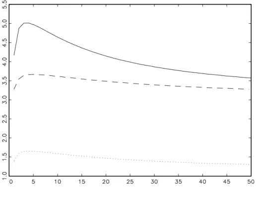
Figure 1 shows the kurtosis and co-kurtosis of the example process (18) as a function of the aggregation level m. Both kurtosis coefficients converge to 3, whereas the co-kurtosis converges to 1 + 2ρ2 = 1.1125. Note however the slow rate of convergence with still substantial excess kurtosis and excess co-kurtosis at m= 50. Moreover, it is remarkable that both kurtosis and co-kurtosis increase for small m. Thus, a series may become even more leptokurtic under temporal aggregation, if the aggregation level is small.
From the weak VARMA representation (35) one obtains the weak VMA(∞) represen-tation ηmt(m)=σ(m)+ ∞ X i=0 Φi(m)u(mm()t−i), (38) where σ(m) = ¡I N −Q(m) ¢−1
ω(m), and where the N ×N matrices Φ(m)
i are given by
Φ0 =IN and
Φ(im)= (Q(m))i−1A(m), i= 1,2, . . . , (39)
4
Causality
There is a substantial literature on the effects of temporal aggregation for causality be-tween time series, see e.g. Marcellino (1999) for a recent overview and references. The general difficulty in empirical work is that only data of the temporally aggregated series is available, for which one typically observes contemporaneous correlation between the series. The question for the investigator is whether this correlation stems from a true causal relation of the high frequency series or whether it is a mere artefact of temporal aggregation. We will address this issue here in the volatility context and show that, again, there are important differences to the VARMA case.
As is common in econometrics, we use the term causality in the sense of ‘Granger causality’, which for volatility has been defined by Granger, Robins, and Engle (1984). However, there are at least three alternative versions of Granger causality, one based on the entire distribution of a variable to be forecast, another on the conditional expecation, and yet another on optimal linear forecasts. Knowing from Section 3 that temporally aggregated multivariate GARCH processes are only weak multivariate GARCH, we have to be careful in defining causality in variance, because notions based on conditional ex-pectations or conditional variances become difficult to check for the aggregated series. Rather, one has to weaken the concept and use the notion of best linear predictors, but this stands in the tradition of, for example, Boudjellaba et al. (1992) and Comte and Lieberman (2000). Also, I use the term ‘Granger causality’ for the case of a causal lag greater than zero (sometimes this is also called ‘directional causality’), whereas I use ‘instantaneous causality’ for the causal lag being actually zero.
Suppose we are interested in the causality in variance between the first two elements of
by εs,i, s ≤ t, i, j = 1,3,4, . . . , K byFt(−2). Moreover, denote by Ht the set of all linear
combinations of a constant andεs,iεs,j,s≤t,i, j = 1, . . . , K (as before in Definition 3), by
H(−2)t the set of all linear combinations of a constant andεs,iεs,j,s≤t,i, j = 1,3,4, . . . , K,
and byH(+2)t the set of all linear combinations of a constant,εs,iεs,j,s≤t,i, j = 1, . . . , K,
and εt+1,2εt+1,i, i= 2, . . . , K.
Definition 4 1. We say that εt,2 Granger causes εt,1 in variance (GCV), denoted by
εt,2 GCV→ εt,1 if, for some h≥1,
Var(εt+h,1 | Ft)6=Var(εt+h,1 | Ft(−2)), (40)
2. There is said to be instantaneous causality in variance (ICV) between εt,2 and εt,1, denoted by εt,1 ICV↔ εt,2 if
Var(εt+1,1 | Ft)6=Var(εt+1,1 | Ft∨σ(εt+1,2)) (41) where Ft∨σ(εt+1,2)denotes the augmentation of Ft−1 by the information contained in εt,2.
3. We say thatεt,2linearly Granger causesεt,1in variance (LGCV), denoted byεt,2 LGCV→
εt,1 if, for some h≥1,
P(ε2
t+h,1 | Ht)6=P(ε2t+h,1 | H (−2)
t ), (42)
4. There is said to be linear instantaneous causality in variance (LICV) between εt,2 and εt,1, denoted by εt,1 LICV↔ εt,2 if
P(ε2
t+1,1 | Ht)6=P(ε2t+1,1 | Ht(+2)) (43)
For weak multivariate GARCH processes it is only possible to investigate linear causal-ity since the conditional variances are not specified or not known. On the other hand, for semi-strong multivariate GARCH processes it is well possible to investigate causality, but that would only be relevant for the high-frequency process. Absence of either of these causality concepts now amounts to zero restrictions on the parameter matrices. Hafner and Herwartz (2004) give necessary and sufficient conditions for absence of GCV and LGCV.
In temporally aggregated VARMA models, Breitung and Swanson (2002) have inves-tigated the effect of so-called spurious instantaneous causality, as first investigated by Renault and Szafarz (1991) and Renault, Sekkat and Szafarz (1998). This occurs if there is no causality between the disaggregated time series, but instantaneous causality between the aggregated time series. We adapt this definition to the volatility case. If there is no causality in volatility (instantaneous or directional) between the series εt,1 and εt,2, we denote this by εt,1 CV= εt,2, and correspondingly we write εt,1 LCV= εt,2 if there is no linear causality in volatility (instantaneous or directional) between the series.
Definition 5 1. There is said to be spurious ICV, if εt,1 CV= εt,2, but ε(mt,m)1
ICV
↔ ε(mt,m)2
for some m≥2 and some t∈Z.
2. There is said to be spurious LICV, if εt,1 LCV= εt,2, but ε(mt,m)1
LICV
↔ ε(mt,m)2 for some
m≥2 and some t∈Z.
It has sometimes been argued that spurious instantaneous causality can be problem-atic in empirical work, since if two aggregated time series are found to show instantaneous causality, it may be because there is causality between the disaggregated series or because it is induced by temporal aggregation. Breitung and Swanson (2003) give sufficient con-ditions to exclude spurious instantaneous causality in VARMA models. In the volatility case, the following theorem gives a necessary condition for spurious instantaneous causal-ity.
Theorem 3 If the high frequency process follows strong multivariate GARCH with Gaus-sian innovations, then a necessary condition for spurious LICV between (εt,1) and (εt,2) is
ht,2 = 0 and K ≥3,
for all t, where ht,2 is the second component of ht, i.e. the conditional covariance of εt,1 and εt,2.
In the following let us be a bit more loose in terminology and only refer to GCV and ICV when it could also mean LGCV or LICV. Theorem 3 implies that in empirical work spurious ICV is of much less relevance than spurious instantaneous causality in the conditional mean, because the two series will in most cases show some non-zero conditional covariance, be it constant or not. Financial series such as stock returns, for example, tend
to be positively correlated at high frequencies. So, ICV will be the rule rather than the exception if high frequency financial series are investigated.
Rather than ICV, it is far more interesting to see whether there is GCV. It turns out that there may be absence of GCV between the disaggregate series, but presence of GCV between the aggregated series. This might be called spurious Granger causality in volatility. A sufficient condition for absence of GCV is that the parameter matrices
A and B of the multivariate GARCH model are diagonal. Many empirical studies have shown that diagonal GARCH models may give good descriptions of the DGP at many frequencies. This can be due to the fact that even though there may be GCV induced by temporal aggregation, it is possibly much less important numerically than ICV. To see whether this is the case for a given multivariate GARCH model, we need measures for the alternative causalities, which we will look at in the following.
Measures for the causality in variance have been considered by Hafner (2003) based on well known measures for causality in VARMA models introduced by Geweke (1982). For simplicity, I only consider the bivariate case in the following, but extensions to causality measures conditional on other variables follow in analogy to Geweke (1984). Letxt=ε2t,1 and yt = ε2t,2. By the results of Nijman and Sentana (1996), the marginal process εt,1 follows a weak univariate GARCH process and therefore xt has a weak ARMA(q∗, p∗)
representation such as xt=ωx+ q∗ X i=1 (αx i +βix)xt−i− p∗ X j=1 βx jwt−j +wt, (44) where wt = xt −P(ε2t,1 | H (−2)
t−1 ), ωx, αxi and βjx are parameters. Upper bounds for the
AR and MA orders are given by q∗ ≤ 3 and p∗ ≤ 3, respectively, by Corollary 4.2.2 of L¨utkepohl (1987) or Nijman and Sentana (1996). The processwtis univariate weak white
noise with variance σ2
w, say. A measure for GCV from yt to xt is given by
GCVy→x = log
σ2
w
[Σu]11
, (45)
By symmetry, one obtains a causality measure for the reverse causality direction,GCVx→y.
Summing up these unidirectional causality measures, we can define a measure for bidi-rectional causality as
A measure for ICV between xt and yt is given by
ICVx↔y = log
Σu,11Σu,33 Σu,11Σu,33−Σ2u,13
, (47)
Finally, the measure for linear dependence betweenxtandytis denoted byCVx,y. This
measure can be decomposed into the three causality measures:
CVx,y =GCVx→y +GCVy→x+ICVx↔y =GCVy↔x+ICVx↔y. (48)
Now suppose one is mainly interested in the bidirectional GCV measure, GCVy↔x,
because, for example, one wants to see how important spurious GCV can become. For example, the hypothesis of a diagonal GARCH model amounts to testing whether this bidirectional measure is zero. For a given multivariate GARCH process there is no obvious way to find the unidirectional measuresGCVy→x andGCVx→y, other than via determining
the univariate GARCH models for the marginal processes, which is straightforward but tedious, see Nijman and Sentana (1996). However, there is a simple way to find the bidi-rectional measureGCVy↔x, as we will see immediately. The measure for linear dependence
can be decomposed in the frequency domain as
CVx,y = 1 2π Z π −π log f11(λ)f33(λ) f11(λ)f33(λ)− |f13(λ)|2 dλ,
see e.g. Geweke (1982), where f(λ) denotes the spectral density matrix ofηt= vech(εtε0t)
which is given by f(λ) = à ∞ X j=0 Φjeijλ ! Σu à ∞ X j=0 Φjeijλ !0 . (49)
The bidirectional measure GCVy↔x can now easily be obtained as a residual of equation
(48), i.e., by the difference between CVx,y and ICVx↔y. The advantage of this approach
is that f(λ) and therefore the bidirectional measure can be calculated directly using the representation of the joint process εt. The alternative way of summing up the two
unidirectional measures requires the determination of the marginal processes εt,1 and εt,2, which is somewhat more involved, see Section 3 of Nijman and Sentana (1996).
The above causality measures can now also be obtained for the aggregated series η(mtm)
by replacing Σu in (49) and (47) by Σ(um) given in (34) and replacing Φi in (49) by Φ(im)
given in (39). This gives us a measure of bidirectional causality in volatility for the aggregated series, defined as
GCV(m)
Since ∀i ≥ 1, Φ(im) → 0 as m → ∞ , the spectral density matrix of the series m−1η(m)
mt
converges to the limit of m−2Σ(m)
u , U say. For example, by the results of Section 2, this
would be given by vec(U) = (cGK −IN2)vec(σσ0) under the assumption of spherical
innovations. Thus, CVx,y(m) and ICVx(m↔)y converge to the same limit given by
lim
m→∞CV (m)
x,y = limm→∞ICVx(m↔)y = log
U11U33
U11U33−U132
Using (50), this implies that limm→∞GCVy(m↔)x = 0, meaning that all directional Granger
causality in variance disappears eventually as the series is aggregated. This is of course no surprise as it corresponds to the aggregation results in VARMA processes.
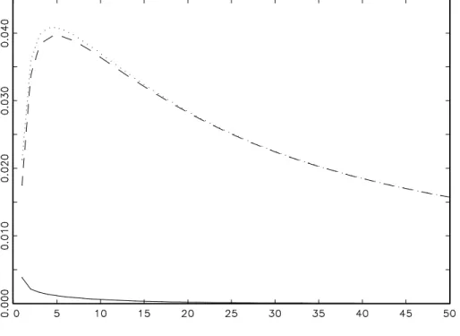
Figure 2 shows the alternative causality measures for the example process (18). Clearly, the bidirectional GCV measure is much smaller here than the ICV measure and also dis-sipates to zero very quickly. Note that the bidirectional GCV measure of the disaggregate process (18) is equal to the unidirectional GCV measure fromεt,2 toεt,1, since the
matri-cesAand B are upper triangular, so that there is no GCV fromεt,1 toεt,2. However, the
bidirectional GCV measure of the aggregated process incorporates some causality from
εt,1 to εt,2, although smaller than from εt,2 to εt,1. But this is not shown in the figure. Finally, the discussed causality measures could be used for testing causality for a given empirical time series. If the errorsut of the VARMA representation of multivariate
GARCH models were Gaussian, then an estimate of the GCV measure, multiplied by the sample size T, would be the usual likelihood ratio statistic, having an asymptotic χ2 distribution, see Geweke (1982). Now ut is not Gaussian but skewed and conditionally
heteroskedastic. Thus, TGCVd could be called pseudo likelihood ratio statistic with a nonstandard asymptotic distribution. To obtain valid critical values one can use the bootstrap as in Hafner and Herwartz (2004). They find that this statistic has similar size and power properties as the so-called CCF test of Cheung and Ng (1996). The CCF test estimates univariate GARCH models and computes cross-correlations of standardized residuals. It is therefore in the spirit of Lagrange Multiplier statistics. A third way to approach the testing problem is to use Wald type statistics, for example based on QML estimation and inference of the multivariate model. Hafner and Herwartz (2004) show that the Wald test has more power under local alternatives than both the CCF and the pseudo likelihood ratio test. However, their framework is a semi-strong multivariate GARCH model and it is as yet unknown whether this carries over to weak GARCH
models. It is related to the problem of estimating weak GARCH models, briefly discussed in Section 7.
5
Forecasting
Suppose one is interested in the prediction of multivariate volatility of the aggregated series h periods ahead. That is, given information at time mt one wants to predict the volatility of ε(mm()t+h). Let us only consider the flow variable case here, so that ε(mm()t+h) =
εm(t+h)+εm(t+h)−1+. . .+εm(t+h−1)+1. Prediction of the volatility ofεm(m()t+h) is the same as prediction ofηm(m(t)+h). One can now build a forecast based on the VMA(∞) representation of the aggregated series in (38). It is given by
ηmt(m)(h) =σ(m)+ ∞
X
i=0
Φh(m+)ium(m()t−i)
The mean square error of this forecast is given by the matrix Σa(h) =
h−1
X
i=0
Φ(im)Σ(um)Φ(im)0.
Another possibility is to predict the disaggregated series and then aggregate the forecasts. Based on the VMA(∞) representation of the disaggregated series in (9), the optimalr-step forecast in a mean square error sense is given by
ηt(r) = σ+
∞
X
i=0
Φr+iut−i
The forecast forηm(m()t+h) is then given byηmt(mh) +ηmt(mh−1) +. . .+ηmt(m(h−1) + 1).
The mean square error of this forecast is given by Σd(h) =FΣdm(h)F0,
whereF = (IN, . . . , IN) is an (N×mN) aggregation matrix, and Σdm(h) is a symmetric,
positive definite (mN ×mN) matrix given by
Σdm(h) = Pm(h−1) i=0 ΦiΣuΦ0i Pm(h−1) i=0 ΦiΣuΦ0i+1 · · · Pm(h−1) i=0 ΦiΣuΦ0i+m−1 Pm(h−1) i=0 Φi+1ΣuΦ0i Pm(h−1)+1 i=0 ΦiΣuΦ0i · · · Pm(h−1)+1 i=0 ΦiΣuΦ0i+m−2 ... ... . .. ... Pm(h−1) i=0 Φi+m−1ΣuΦ0i Pm(h−1)+1 i=0 Φi+m−2ΣuΦ0i · · · Pmh−1 i=0 ΦiΣuΦ0i ,
see e.g. chapter 8 of L¨utkepohl (1987). There it is also shown that for VARMA models in general Σd(h) ≤ Σa(h) in the sense that the matrix Σa(h)−Σd(h) is positive
semi-definite, and that equality only holds in special cases such as periodicity with period equal to the aggregation level. An implication of this result is that the forecasts based on the disaggregated series are superior to the forecasts based on the aggregated series in terms of forecast precision. On the other hand, both forecasts become equivalent as the forecast horizon increases, as both mean square error matrices approach the same unconditional covariance matrix.
For the aggregation of multivariate GARCH processes, however, the difference between both forecasts turns out to be stronger than for VARMA processes and not dissipating for increasing horizons. The reason is the additional noise term in the aggregated series,
w(mtm). The expectation of this term is zero, but it has a positive definite covariance matrix Σ(wm) given by (22). Therefore, the unconditional variance of ηmt(m) is larger than that of
ηmt+ηmt−1+. . .+ηm(t−1)+1, and the forecast mean square error matrices converge to two different levels with increasing horizon. Thus, we have a strict inequality, Σd(h)<Σa(h)
for all h >0. Asymptotically, the difference is given by lim
h→∞Σa(h)−Σd(h) = Σ (m)
w , (51)
where Σ(wm) is given by (22). As the difference between the two forecasting methods is
negligible in VARMA models for sufficiently large horizons, it turns out to be substantial in multivariate GARCH models. Equation (51) says that in the limit this difference is just given by the variance matrix of the noise term w(mtm) in (21) that was added to the sum of the indivual ηmt in constructing the aggregate ηmt(m). It should be emphasized
that this noise term is missing in the aggregation of VARMA processes. The implication of (51) is that forecasting weekly volatility, for example, by aggregating daily volatility forecasts will always be better than forecasting the weekly series directly, no matter how large the forecasting horizon. This is also the reason why in forecasting volatility one should use the highest frequency for which data is available, provided that there are no biases coming from microstructure effects, for example. Recent empirical research has shown that predicting daily volatility of a financial time series using intra-day returns can substantially improve the precision of forecasts using the daily series only, see e.g. Andersen et al. (2003). See also Section 6, where this so-called realized volatility is investigated in the context of multivariate GARCH models.
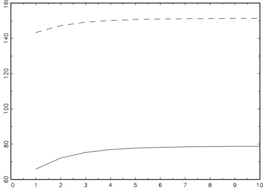
Figure 3 shows the mean square prediction errors of the two forecasting methods for the example process (18) with m = 2. In this example, the mean square prediction error can be reduced by almost 50 % for all forecasting horizons by doubling the sampling frequency and using the high frequency data for prediction.
6
Multivariate realized volatility
There is a growing literature on so-called realized volatilities, see, e.g., Andersen et al. (2003) for an overview. Realized volatilities are estimates of low-frequency volatilities using high frequency data. For example, the volatility of a daily return series could be estimated by the sum of squared intra-day returns. When the sampling frequency goes to infinity, realized volatilities converge to the actual volatility and are therefore consistent, unbiased estimates of daily volatility. In the multivariate context, the same idea applies to the vector of squares and cross-products,ηt = vech(εtε0t). The aggregation scheme is no
longerε(mtm) =εmt+εmt−1+. . .+εmt−m+1 but ¯ηmt=ηmt+ηmt−1+. . .+ηmt−m+1. Thus, all the cross-terms that appeared in our previous aggregation scheme η(mtm) = vech(εmt(m)ε(mtm)0) are absent here.
First, it is clear that for any finite m, ¯ηmt is an unbiased estimate of the unobservable
daily volatility. It is more efficient than the noisy η(mtm) = vech(εmt(m)ε(mtm)0) but, for every finite m it is inefficient compared to ¯hmt = hmt+hmt−1 +. . .+hmt−m+1. The practical advantage of using ¯ηmt is, of course, that no parametric model of volatility needs to be
specified, but a drawback is given by the restriction thatm can not be chosen arbitrarily large. In other words, the time interval between observations can not be arbitrarily small due to market microstructure effects. If the true volatility process follows multivariate GARCH, we quantify below the loss of efficiency of ¯ηmt compared with ¯hmt.
To calculate the variance of ¯ηmt, note that this is just the sum of the variances of the
individual terms ηmt, each one equal to Ση−σσ0, plus the sum of all covariances. This is
given by
Var(¯ηmt) =m(Ση−σσ0) + mX−1
i=1
(m−i) (Γ(i) + Γ(i)0).
Similarly, we obtain for the variance of ¯hmt
Var(¯hmt) =m(Σh−σσ0) + mX−1
i=1
so that the difference is given by
Var(¯ηmt)−Var(¯hmt) =m(Ση −Σh), (53)
which is positive semi-definite. Note that (52) is O(m2) and (53) is O(m), so that the relative difference between the two variances is O(m−1). In other words, the loss of effi-ciency of realized volatilities w.r.t. the model (supposing that this is correctly specified) is diminishing with rateO(m−1). In practice,m can not increase without bounds, so that the relative efficiency for a given m depends on features such as the volatility persistence and the correlation. Let us define the relative efficiency of the i-th component of real-ized volatility w.r.t. the model as the i-th diagonal element of Var(¯ηmt) divided by the
corresponding diagonal element of Var(¯hmt), that is,
REi(m) = [Var(¯ηmt)]ii £ Var(¯hmt) ¤ ii . (54)
Note that REi(m) = 1 +O(m−1) so that for m sufficiently large the efficiency loss is
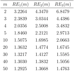
negligible. However, if m can not be chosen arbitrarily large in practice, the efficiency loss may be substantial. For our example process (18), Table 1 lists the values of REi(m)
for selected levels m. Obviously, even at m = 50 the variance of the realized volatility estimator is still 29% higher than that of the optimal one for the first component of
η(mtm). For the other two components the loss is even higher. For their exchange rate example, Andersen et al. (2003) use a value of m = 48, having half-hourly data for a 24 hours per day market. They can not choose m much larger because of the problems with interfering microstructure effects such as bid-ask bounces. The values ofREi(m) in
Table 1 therefore appear relevant if our example process can be considered as a typical high frequency process. In such a situation the practitioner has to weigh the risk of mis-specifying a parametric volatility model for the high frequency process against the efficiency loss of the nonparametric estimation using realized volatilities.
There is a second issue concerning standardized residuals using realized volatilities which turns out to be intimately related to the relative efficiency issue. Standardized residuals are typically obtained by ¯Hmt−1/2εmt(m), where ¯Hmt is the de-vectorized ¯hmt, for
the given multivariate GARCH model. Alternatively, without an assumption on the underlying process, one can define standardized residuals by Υ−1mt/2ε(mtm), where Υmt is the
m RE1(m) RE2(m) RE3(m) 2 3.2264 4.3470 6.8479 3 2.3839 3.0344 4.4386 4 2.0356 2.5008 3.4832 5 1.8460 2.2121 2.9713 10 1.5075 1.6985 2.0663 20 1.3632 1.4774 1.6745 30 1.3217 1.4127 1.5585 40 1.3030 1.3832 1.5056 50 1.2925 1.3668 1.4763
Table 1: Relative efficiencies according to definition (54) of realized volatilities with respect to the optimal estimates when the high frequency process is known to be the process given in (18). RE1 is the measure for the conditional variance of ε(mt,m)1, RE2 is the measure for the conditional covariance of ε(mt,m)1 and εmt,(m)2, and RE3 is the measure for the conditional variance of ε(mt,m)2.
residuals standardized by realized volatilities ¯ηmt will be smaller than that of residuals
standardized by ¯hmt. In particular, if the innovation distribution is Gaussian, the kurtosis
of the residuals standardized by realized volatilities is smaller than three, which is also apparent in the empirical results of Andersen et al. (2003), Table 1. They claim that standardized residuals are close to being Gaussian, but for their sample of ten years of daily returns on the DM/Dollar exchange rate a value of 2.57 for the kurtosis of standardized residuals is likely to violate the normality assumption.4 It can also be shown that, using first order expansions, the negative bias of the kurtosis estimate is directly related to the efficiency loss expressed by REi(m).
Recently, interest has focused on the distribution of realized volatilities. If the true underlying DGP is multivariate GARCH andm is sufficiently large, this may be approxi-mated by the asymptotic distribution of the centered and normalized realized volatilities,
4This can be seen by noting that for an i.i.d. Gaussian white noise, the standard error of the kurtosis
estimator is (24/n)1/2, wherenis the sample size. Ifn= 2500, which roughly corresponds to ten years
of daily data, the standard error takes the value 0.098, so that with an estimate of 2.57 one would reject the null hypothesis of Gaussian white noise at the 95% significance level.