Collocation Orthonormal Berntein Polynomials method for Solving Integral Equations

Collocation Orthonormal Berntein Polynomials method for

Solving Integral Equations.

Suha. N. Shihab; Asmaa. A. A.; Mayada. N.Mohammed Ali University of Technology Applied Science Department Abstract:

In this paper, we use a combination of Orthonormal Bernstein functions on the interval [0,1] for degree

𝑚 = 5,and 6 to produce anew approach implementing Bernstein Operational matrix of derivative as a method for the numerical solution of linear Fredholm integral equations of the second kind and Volterra integral equations. The method converges rapidly to the exact solution and gives very accurate results even by low value of m. Illustrative examples are included to demonstrate the validity and efficiency of the technique and convergence of method to the exact solution.

Keywords: Bernstein polynomials, Operational Matrix of Derivative, Linear Fredholm Integral Equations of the Second Kind and Volterra Integral Equations.

1. Introduction:

In the Survey of solutions of integral equations, a large number of analytical but afew approximate methods for solving numerically various classes of integra equations [1]. Orthogonal functions and polynomial series have received considerable attention in dealing with various problems of dynamical Systems. The main Characteristic of this technique is that it reduces these problems to those of solving a system of algebraic equations, thus greatly simplifying the problem [2,14]. While in recent years interest in the solution of integral and differential equations, such as Fredholm, Volterra, and integro-differential equations [3]. The general form of Fredholm, Volterra integral equations respectively are

1-

𝑢(𝑥) = 𝑔(𝑥) + ∫ 𝑘(𝑥, 𝑡)𝑢(𝑡)𝑑𝑡 𝑥 ∈ [0,1]₀1 (1)

2-

𝑢(𝑥) = 𝑓(𝑥) + ∫ 𝑘(𝑥, 𝑡)𝑢(𝑡)𝑑𝑡 𝑥 ∈ [0,1]₀𝑥 (2)

Integral equations are widely used for solving many problems in mathematical physics and engineering. In recent years, many different basic functions have been used to estimate the solution of integral equations, such as Block-Pulse functions [4,5], Hybrid Legendre and Block-Pulse functions. Bernstein polynomials play a promineut role in various areas of mathematics. These polynomials, have been frequently used in the solution of integral equations,differential equations and approximation theory,see [6]. Recently the various operational matrices of the polynomials have been developed to cover the numerical solution of differential, integral and integro-differential equations. In [7] the operational matrices of Bernstein polynomials are introduced. Doha [8] has drived the shifted Jacobi operational matrix of fractional derivatives which is applied together with the Spectral Tau method for the numerical solution of dynamical systems.Yousefi et al.in [9], [10] and [11] have presented Legendre wavelets and Berntein operational matrices and used them to solve miscellaneous systems. Lakestani et al. [12] constracted the operational matrix of fractional derivatives using B-Spline functions. Another motivation is concerned with the direct solution techniques for solving the Fredholm and Volterra integral equations respectively on the interval [0,1] using the method based on the derivatives of orthonormal (B-polynomials) sense for m=5 and 6. Finally, the accuracy of the proposed algorithm is demonstrated by test problems.

2-Bernstein Polynomials (B-Polynomials):

The Bernstein polynomias (B-Polynomials) [13], are some usfel polynomials defined on [0,1]. The Bernstein Polynamials of degree m form a basis for the power polynomials of degree m. we can mentioned, B-Polynomials are aset of B-Polynomials

Note that each of these m+1 Polynomials having degree m is normalization, i.e

∑𝑚𝑘=0𝐵𝑘,𝑚(𝑥) = 1, has one root, each of multiplicity k and m-k, at x=0 and x=1 respectively,also 𝐵𝑘,𝑚(𝑥) in which 𝑘{0, 𝑚}has asingle unique local maximum of 𝑘_𝑚𝑘−𝑚(𝑚 − 𝑘)𝑚−𝑘(𝑚_{𝑘 )}, it can provide flexibility applicable to impose boundary conditions at the end points of the interval. First derivatives of the generalized Bernstein basis polynomials.

_𝑑𝑥𝑑 𝐵𝑘,𝑚(𝑥) = 𝑚[𝐵𝑘−1,𝑚−1(𝑥) + 𝐵𝑘,𝑚−1(𝑥)] (4) In this paper, we use 𝑚(𝑥) notation to show

𝑚(𝑥) = [𝐵0𝑚(𝑥), 𝐵1𝑚(𝑥), … , 𝐵𝑚𝑚(𝑥)]𝑇 (5) where we can have

𝑚(𝑥) = 𝐴𝑚(𝑥)∆𝑚(𝑥) (6)

that A is the matrix and (𝑘 + 1)𝑡ℎ row of A is

𝐴𝑘+1= [0,0, …𝑘 𝑡𝑖𝑚𝑒𝑠, 0, 𝑠_(0, 𝑘, 𝑚), 𝑠_(1, 𝑘, 𝑚), … , 𝑠_(𝑚, 𝑘, 𝑚) ] =[0,0, …𝑘 𝑡𝑖𝑚𝑒𝑠, 0, (−1)0(𝑚_{𝑘 ) (}𝑚 − 𝑘 0 ) , (−1)1( 𝑚 𝑘 ) (𝑚 − 𝑘1 ) , … , (−1)𝑚−𝑘( 𝑚 𝑘 ) (𝑚 − 𝑘𝑚 − 𝑘)] (7) where 𝑆𝑖,𝑘,𝑚= (−1)𝑖(𝑚_{𝑘 ) (}𝑚 − 𝑘_𝑖 ) and ∆𝑛(𝑥) = [ 𝑥0 𝑥1 ⋮ 𝑥𝑚 ] (8)

using MATHEMATICA code, the first six (B-Polynomials) of degree five over the interval [0,1], are given

𝐵05(𝑥) = (1 − 𝑥)5 𝐵15(𝑥) = 5𝑥(1 − 𝑥)4 𝐵25(𝑥) = 10𝑥2(1 − 𝑥)3 𝐵35(𝑥) = 10𝑥3(1 − 𝑥)2 𝐵45(𝑥) = 5𝑥4(1 − 𝑥) 𝐵55(𝑥) = 𝑥5

and the first seven (B-Polynomials) of degree six over [0,1] are given

𝐵06(𝑥) = (1 − 𝑥)6 𝐵16(𝑥) = 6𝑥(1 − 𝑥)5 𝐵26(𝑥) = 15𝑥2(1 − 𝑥)4 𝐵36(𝑥) = 20𝑥3(1 − 𝑥)3 𝐵46(𝑥) = 15𝑥4(1 − 𝑥)2 𝐵56(𝑥) = 6𝑥5(1 − 𝑥) 𝐵66(𝑥) = 𝑥6

3-

A function u(x) equation, square integrable in (0,1), many be expressed in terms of Bernstein basis [7]. In practice, only the first (m+1)-terms Bernstein polynomials are considered. Hence if we write

𝑢(𝑥) ≈ ∑𝑚𝑘=0𝑐𝑘𝐵𝑘𝑚(𝑥) = 𝐶𝑇(𝑥) (9) where 𝑇(𝑥) = [𝐵_0𝑚(𝑥), 𝐵_1𝑚(𝑥), … , 𝐵_𝑚𝑚(𝑥)] and

𝐶𝑇= [𝑐₀, 𝑐₁, … , 𝑐_𝑚] can be calculated by:

𝐶𝑇= (∫ 𝑢(𝑥)∅₀1 𝑇(𝑥)𝑑𝑥) 𝑄−1, (10)

where 𝑄 is an (𝑚 + 1) × (𝑚 + 1) matrix and is said dual matrix of (𝑥)

𝑄(𝑥) = ((𝑥),(𝑥)) = ∫ ∅(𝑥) ∅1 𝑇_{(𝑥)𝑑𝑥} 0 =∫ (𝐴∆𝑛(𝑥))(𝐴∆𝑛(𝑥)) 𝑇 𝑑𝑥 1 0 = 𝐴 [∫ ∆₀1 𝑛(𝑥)∆𝑛𝑇(𝑥)𝑑𝑥] 𝐴𝑇 = 𝐴𝐻𝐴𝑇, (11) A is defined by eqs.(7) and H is a Hilbert matrix

𝐻 = [ 1 12 … 1 𝑚+1 1 2 1 3 … 1 𝑚+2 ⋮ ⋮ ⋱ ⋮ 1 𝑚+1 1 𝑚+2 … 1 2𝑚+1] and 𝑄 = [ 𝑄1 0 … 0 0 𝑄2 … 0 ⋮ ⋮ ⋱ ⋮ 0 0 … 𝑄𝑚 ]

The elements of the dual matrix 𝑄, are given explicity by

(𝑄𝑚)𝑘+1,𝑖+1= ∫ 𝐵₀1 𝑘𝑚(𝑥)𝐵𝑖𝑚(𝑥)𝑑𝑥

= (𝑚_{𝑘 ) (}𝑚_{𝑖 ) ∫ (1 − 𝑥)0}1 2𝑚−(𝑘+𝑖)𝑥𝑘+𝑖𝑑𝑥 (12) where 𝑘, 𝑖 = 0,1, … , 𝑚

4-

The representation of the orthonormal Bernstein Polynomials, denoted by 𝑏_𝑖5(𝑥), 𝑏_𝑖6(𝑥) here, was discovered by analyzing the resulting orthonormal polynomials after applying the Gram-Schmidt process on sets of Bernstein polynomials of degree five and six.

We get the following sets of orthonormal polynomials [10],[11].

𝑏05(𝑥) = √11(1 − 𝑥)5

𝑏15(𝑥) = 6 [5𝑡(1 − 𝑥)4−1₂(1 − 𝑥)5]

𝑏25(𝑥) =18√7₅ [10(1 − 𝑥)3𝑡2− 5(1 − 𝑥)4𝑡 +₁₈5 (1 − 𝑥)5]

𝑏45(𝑥) = 7√3 [5(1 − 𝑥)𝑥4− 20(1 − 𝑥)2𝑥3+ 18(1 − 𝑥)3𝑥2− 4(1 − 𝑥)4𝑥 +1₇(1 − 𝑥)5] 𝑏55(𝑥) = 6 [𝑥5−25₅ (1 − 𝑥)𝑥4+100₃ (1 − 𝑥)2𝑥3− 25(1 − 𝑥)3𝑥2+ 5(1 − 𝑥)4𝑥 −1₆(1 − 𝑥)5] and 𝑏06(𝑥) = √13(1 − 𝑥)6 𝑏16(𝑥) = √44 [6𝑡(1 − 𝑥)5−1₂(1 − 𝑥)6] 𝑏26(𝑥) = 11 [15(1 − 𝑥)4𝑥2− 6(1 − 𝑥)5𝑥 +₁₁3 (1 − 𝑥)6] 𝑏36(𝑥) = √252 [20(1 − 𝑥)3𝑥3−45₂(1 − 𝑥)4𝑥2+ 5(1 − 𝑥)5𝑥 −11₆₆(1 − 𝑥)6] 𝑏46(𝑥) =_√542[15(1 − 𝑥)2𝑥4− 40(1 − 𝑥)3𝑥3+180₇ (1 − 𝑥)4𝑥2−30₇(1 − 𝑥)5𝑥 +₄₂5 (1 − 𝑥)6] 𝑏56(𝑥) =_√328[6𝑡5(1 − 𝑥) −75₂(1 − 𝑥)2𝑥4+ 60(1 − 𝑥)3𝑥3− 30(1 − 𝑥)4𝑥2+30₇ (1 − 𝑥)5𝑥 −₂₈3 (1 − 𝑥)6] 𝑏66(𝑥) = 7 [𝑥6− 18(1 − 𝑥)𝑥5+ 75(1 − 𝑥)2𝑥4− 100(1 − 𝑥)3𝑥3+ 45(1 − 𝑥)4𝑥2− 6𝑡(1 − 𝑥)5+ 1 7(1 − 𝑥) 6_]

In addition, we have determind the explicit representation for the orthonormal Bernstein polynomials as [16]

𝑏𝑘𝑚(𝑥) = (√2(𝑚 − 𝑘) + 1) (1 − 𝑥)𝑚−𝑘∑𝑘𝑖=0(−1)𝑖(2𝑚 + 1 − 𝑖_{𝑘 − 𝑖} ) (𝑘_𝑖) 𝑥𝑘−𝑖 (13)

The eqs(13) can be written in terms of the Bernstein basis functions as

𝑏𝑘𝑚(𝑥) = (√2(𝑚 − 𝑘) + 1) ∑ (−1)𝑖 (2𝑚+1−𝑖 𝑘−𝑖 )(𝑘𝑖) (𝑚−𝑖 𝑘−𝑖) 𝐵𝑘−𝑖,𝑚−𝑖(𝑥) 𝑘 𝑖=0 (14)

Any generalized Bernstein basis polynomials of degree m can be wretten as a linear combination of the generalized Bernstein basis polynomials of degree m+1

𝐵𝑘,𝑚(𝑥) =𝑚−𝑘+1_𝑚+1 𝐵𝑘,𝑚+1(𝑥) +_𝑚+1𝑘+1𝐵𝑘+1,𝑚+1(𝑥) (15)

By utilizing eqs(15),the following functions can be written as

𝐵𝑘,𝑚−1(𝑥) =𝑚−𝑘_𝑚 𝐵𝑘,𝑚(𝑥) +𝑘+1_𝑚 𝐵𝑘+1,𝑚(𝑥) (16)

and

𝐵𝑘−1,𝑚−1(𝑥) =𝑚−𝑘+1_𝑚 𝐵𝑘−1,𝑚(𝑥) +_𝑚𝑘𝐵𝑘,𝑚(𝑥) (17)

Substituting these eqs(16) and (17) into the right hand side of the eqs(4), we get the following derivatives of Bernstein basis polynomials

𝑑

𝑑𝑥𝐵𝑘,𝑚(𝑥) = (𝑚 − 𝑘 + 1)𝐵𝑘−1,𝑚(𝑥) + (2𝑘 − 𝑚)𝐵𝑘,𝑚(𝑥) − (𝑘 + 1)𝐵𝑘+1,𝑚(𝑥) (18) In [10], the derivative of the orthonormal (B-Polynomials)of degree five are introducedas given

𝑏05′ = [−5√11 𝐵05− √11𝐵15]

𝑏15′ = [45𝐵05− 15𝐵15− 2𝐵25]

𝑏35′ = [145_√5𝐵05−235_√5𝐵15+_√578𝐵25+154_√5𝐵35−113_√5𝐵45]

𝑏45′ = [−33√3𝐵05+331√3₅ 𝐵15−217₅ 𝐵25126√3₅ 𝐵35+ 77√3𝐵45− 35√3𝐵55]

𝑏55′ = [35𝐵05− 55𝐵15+ 63𝐵25+ 35𝐵35− 119𝐵45+ 105𝐵55]

and we introduce the derivative of the orthonormal (B-Polynomials) for degree six

𝑏06′ = [−6√11 𝐵06− √13𝐵16] 𝑏16′ = [8√11𝐵06− 7√11𝐵16− 4√11𝐵26] 𝑏26′ = [−84 𝐵06+ 96𝐵16+ 𝐵26− 3𝐵36] 𝑏36′ = [36√7𝐵06− 64√7𝐵16+ 32√7𝐵26+ 27√7𝐵36− 24√7𝐵46] 𝑏46′ = [−42√5𝐵06+ 95√5𝐵16− 150.263681𝐵26− 40.24922359𝐵36+ 187.8297101𝐵46− 42√5𝐵56] 𝑏56′ = [46√3𝐵06− 206.1140461𝐵16+ 235.5589098𝐵26− 14√3𝐵36− 242.4871131𝐵46+ 266.7358244𝐵56− 56√3𝐵66] 𝑏66′ = [−48𝐵06+ 132𝐵16− 168𝐵26+ 42𝐵36+ 168𝐵46− 252𝐵56+ 168𝐵66] 5. Second kind integral equations:

In this section, we use Orthonormal Polynomials for solving second kind Fredholm and Volterra integral equations.

1- Fredholm integral equation (FIE):

Where in eq(1) 𝑔(𝑥) ∈ 𝐿2[0,1], 𝑘(𝑥, 𝑡) ∈ 𝐿2([0,1] × [0,1]) are known and 𝑢(𝑡) is unknown function to be determined.

First we assume the unknown functions

𝑢_𝑖(𝑥) = 𝐶_𝑖𝑇𝐵(𝑥), 𝑖 = 1,2, … , 𝑛 (19) by substituting (19)in (1) we have:

𝐶𝑖𝑇𝐵(𝑥) = 𝑔𝑖(𝑥) + ∫ 𝑘𝑖,𝑗(𝑥, 𝑡) 1 0 𝐶𝑖𝑇𝐵(𝑡)𝑑𝑡 𝐶_𝑖𝑇𝐵(𝑥) − ∫ 𝑘₀1 _𝑖,𝑗(𝑥, 𝑡)𝐶_𝑖𝑇𝐵(𝑡)𝑑𝑡 = 𝑔_𝑖(𝑥) (20) Pick distinct node points 𝑡1, 𝑡2, … , 𝑡𝑛∈ [0,1]

This leads to determining { 𝑐₁, 𝑐₂, … , 𝑐_𝑛} as the solution of linear system

∑𝑛𝑖=1𝐶𝑗[𝐵(𝑥𝑖) − ∫ 𝑘(𝑥₀1 𝑗, 𝑡𝑖)𝐵(𝑡𝑖)𝑑𝑡] = 𝑔(𝑥𝑖) (21)

In this paper Collocation points are 𝑡𝑖=_𝑛𝑖 𝑓𝑜𝑟 𝑖 = 1,2, … , 𝑛 so that we have a system of linear equations 𝐿𝑛𝑋 = 𝑙𝑛 where 𝐿𝑛= |𝐵(𝑥𝑖) − ∫ 𝑘(𝑥₀1 𝑗, 𝑡𝑖)𝐵(𝑡𝑖)𝑑𝑡| 𝑖=0 𝑛 𝑗 = 1,2, … , 𝑛 𝑙𝑛= [𝑔(𝑥𝑖)], 𝑖 = 𝑜, 1, … , 𝑛

2- Volterra integral equation (VIE):

Similarly above section by using Collocation points 𝑡_𝑖= 𝑖

𝐿𝑛= |𝐵(𝑥𝑖) − ∫ 𝑘(𝑥₀𝑥 𝑗, 𝑡𝑖)𝐵(𝑡𝑖)𝑑𝑡|_𝑖=0 𝑛

𝑗 = 1,2, … , 𝑛

𝑙𝑛= [𝑓(𝑥𝑖)], 𝑖 = 𝑜, 1, … , 𝑛 6.Numerical Results:

In this section VIE, FIE is considered and solved by the introduced method. Example 1: Consider the following FIE

𝑢(𝑥) = sin 𝑥 + ∫ (1 − 𝑥 cos 𝑥𝑡) 𝑢(𝑡)𝑑𝑡₀1 (22) the exact solution u(x)=1. Solving eqs(20) and (21) we get the values of 𝐶 𝑇

𝐶=[0.91402903 0.10091438 3.48867166 −2.7619172 3.51373945 0. 15379915 0.98896685]𝑇 Table1 shows the numerical results for this example.

Table 1:some numerical results for example 1 x Approximat solution 𝑏_𝑛(𝑥) Approximat solution 𝐵_𝑛(𝑥) 𝐴𝑏𝑠𝑜𝑢𝑡𝑒𝐸𝑟𝑟𝑜𝑟 |𝑒𝑥𝑎𝑐𝑡 − 𝐵𝑛6| 0 0.91402333 0.99993256 6.7440e-005 0.1 0.93422123 0.99993267 6.7330e-005 0.2 0.96878356 0.99994532 5.4680e-005 0.3 0.96878320 0.99994444 5.5560e-005 0.4 0.97843933 0.99995324 4.6760e-005 0.5 0.93270466 0.99995417 4.5830e-005 0.6 0.99388042 0.99996618 3.3820e-005 0.7 0.99963715 0.99997654 2.3460e-005 0.8 0.98888323 0.99998790 1.2100e-005 0.9 0.99999668 0.99999999 1.0000e-008 1 0.99999998 1.00000000 0.00000000 𝑀. 𝑆. 𝐸 =6.7440e-005 𝐿. 𝑆. 𝐸=2.1286e-008

Example 2: Consider the following FIE

𝑢(𝑥) = 𝑒−𝑥_{− ∫ 𝑥𝑒}1 𝑡_{𝑢(𝑡)𝑑𝑡} 0

the exact solution 𝑢(𝑥) = 𝑒−𝑥−𝑥

2. Solving eqs(20) and (21) we get the values of 𝐶 𝑇

𝐶=[1 1.13944655 −0.05603088 0.85196593 −0.13491534 0. 11655846 − 0.16383600]𝑇 Table2 shows the numerical results for this example.

Table2:some numerical results for example 2 x

Exact solution Approximat solution 𝑏𝑛(𝑥) Approximat solution 𝐵𝑛(𝑥) 𝐴𝑏𝑠𝑜𝑢𝑡𝑒𝐸𝑟𝑟𝑜𝑟 |𝑒𝑥𝑎𝑐𝑡 − 𝐵𝑛6| 0 1 1 1 0.00000000 0.1 0.85483742 0.94188967 0.85488967 0.00005225 0.2 0.71873075 0.76843118 0.71811760 0.00008101 0.3 0.59081822 0.59503874 0.59081874 0.00000052 0.4 0.47032005 0.46240281 0.47032115 0.00000110 0.5 0.35653066 0.35230187 0.35653066 0.00352200 0.6 0.24881164 0.24605093 0.24880053 0.00001111 0.7 0.14658530 0.13907957 0.14658510 0.00000020 0.8 0.04932896 0.04047384 0.04932895 0.00000001 0.9 -0.04343034 -0.04663478 -0.04343155 0.00000121 1 -0.13212056 -0.16383600 -0.13212056 0.00000000 𝑀. 𝑆. 𝐸 =0.00352200 𝐿. 𝑆. 𝐸=0.00000000 Fig1 of example1 0 0.1 0.2 0.3 0.4 0.5 0.6 0.7 0.8 0.9 1 -0.2 0 0.2 0.4 0.6 0.8 1 1.2 exact Bn6

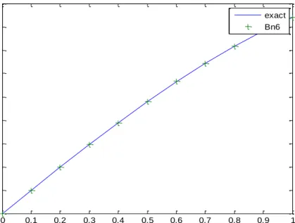
Fig 2 of example3

Example 3: Consider the following VIE

𝑢(𝑥) = 𝑥 − ∫ (𝑥 − 𝑡)𝑢(𝑡)𝑑𝑡₀𝑥 (23) The exact solution 𝑢(𝑥) = sin 𝑥. Table(3) shows the numerical results for this example(3)

𝐶=[0 0.15606151 0.37680718 0.40682330 0.73751386 0. 68080388 0.84172197]𝑇

Table3:some numerical results for example 3 x

Exact solution Approximat solution 𝑏𝑛(𝑥) Approximat solution 𝐵𝑛(𝑥) 𝐴𝑏𝑠𝑜𝑢𝑡𝑒𝐸𝑟𝑟𝑜𝑟 |𝑒𝑥𝑎𝑐𝑡 − 𝐵𝑛6| 0 0.00000000 0.00000000 0.00000000 0.00000000 0.1 0.09983342 0.09924030 0.09983389 0.00000059 0.2 0.19866933 0.19972478 0.19865878 0.00001055 0.3 0.29552021 0.29617066 0.29552053 0.00000065 0.4 0.38941834 0.38930420 0.38941820 0.00000014 0.5 0.47942554 0.47990931 0.47942560 0.00000048 0.6 0.56464247 0.56604342 0.56604342 0.00140095 0.7 0.64421769 0.64342047 0.64342047 0.00007972 0.8 0.71735609 0.70896119 0.71732785 0.00008394 0.9 0.78332691 0.76751046 0.78331110 0.00001581 1 0.84147098 0.84172197 0.84147073 0.00000025 𝑀. 𝑆. 𝐸 =0.00140095 𝐿. 𝑆. 𝐸=0.00000000 0 0.1 0.2 0.3 0.4 0.5 0.6 0.7 0.8 0.9 1 0 0.1 0.2 0.3 0.4 0.5 0.6 0.7 0.8 0.9 exact Bn6

Conclusion:

In this work, VIE,FIE have been solved by using Bernstein basis polynomials of degree m in collocation method. Comparison of the approximate solutions and the exact solutions show that the proposed method is efficient tool. Illustrative examples are included to demonstrate the validity and applicability of the technique.

References:

1. S.Swarup,”Integral equations (Krishna Prakanshan Media Prt.Ltd,15th Editions,2007).

2. Shihab. S. N. and Asmaa. A. A. 2012. Numerical Solution of Calculus of Variations by using the Second Chebyshev Wavelets, Eng. & Tech. Journal. 30(18): 3219-3229.

3. H. Goghary. H. Goghary. M,”Tow Computational methods for Solving linear Fredholm fuzzy integral equations of the Second kind”, APPl. Math. Comput, Vol 182, PP. 791-794, 2006.

4. K. Maleknejad, S.Sohrab1, B. Bevenj1-,”Application of D-BPFS to nonlinear integral equation”, Commun Non linear Sci Number Simulat, 15,PP. 527-535,2010.

5. K.Maleknejad, M.Mordad, B.Raimi,”Anumerical method to solve Fredholm Volterra integral equations two dimensional spaces using Block Pulse Functions and operational Matrix “, Journal of Computational and Applied Mathematics, 2010.

6. E. H.Doha, A.H.Bhrawy, M.A.Saher, “On the derivatives of Bernstein Polynomials: An application for the Solution of high even-order differential equations, Boundary Value Problems Vol, 2011, Article I D & 29543,16 pages doi: 10.1155/2011/829543,2011.

7. S. A. Yousefi, M. Behroozifar, “Operational matrices of Bernstein Polynomials and their applications, Int. J. Syst.Sci.41 (6) (2010) 709-716.

8. E. H. Doha and A. H. Bhrawy S. S. Ezz-Eldien, “Anew Jacobi Operational matrix: An Application for Solving frastional differential equations”, Appl. Math. Model. 36, pp. 4931-4943 2012.

9. S. A. Yousefi and H. Jafari and M. A. Firooz jaecard. S. Momani and C.M.Khaliqued, “Application of Legendre wavelets for solving fractional differential equations, “Comput. Math. Appl. 62, 1038-1045 (2011). 10. S. A. Yousefi and M.Behroozifar and M. Dehghan, “Numerical Solution of the nonlinear age-structured population models by using the operational matrices of Bernstein polynomials”, Appl. Math. Modell. 36, 945-963 (2012).

11. S.A.Yousefi and M. Behroozifar and M. Dehghan, “ The Operational matrices of Bernstein Polynomials for Solving the Parabolic equation subject to specification of the ma ss, J. Comput. Appl.Math. 335, 5272-5283 (2011).

12. Lakestani, M, Dehghan, M, Irandoust-Pakchin, S: ” The Construction of Operational matrix of

fractional derivatives using B-Spline functions”, Commun Nonlinear Sci Number simulat. 17, 1149-1162 (2012). 13. Vineet Kumar Singh, Eugene B. Postnikov, “ Operational matrix approach for solution of integro-differential equations arising in theory of an omalous relaxation processes in Vicinity of singular point”, Applied Mathematical Modelling 37,(2013), 6609-6619.

14. Asmaa. A. A. 2014. Numerical solution of Optimal problems using new third kind Chebyshev Wavelets Operational matrix of integration, Eng. & Tec. Journal. 32(1):145-156.