Handling Missing Values with Regularized Iterative
Multiple Correspondence Analysis
Julie Josse, Marie Chavent, Benoit Liquet, Fran¸cois Husson
To cite this version:
Julie Josse, Marie Chavent, Benoit Liquet, Fran¸cois Husson. Handling Missing Values with
Regularized Iterative Multiple Correspondence Analysis. Journal of Classification, Springer
Verlag, 2012, 29 (1), pp.91-116.
<
10.1007/s00357-012-9097-0
>
.
<
hal-00763227v3
>
HAL Id: hal-00763227
https://hal.archives-ouvertes.fr/hal-00763227v3
Submitted on 19 Dec 2012
HAL
is a multi-disciplinary open access
archive for the deposit and dissemination of
sci-entific research documents, whether they are
pub-lished or not.
The documents may come from
teaching and research institutions in France or
abroad, or from public or private research centers.
L’archive ouverte pluridisciplinaire
HAL
, est
destin´
ee au d´
epˆ
ot et `
a la diffusion de documents
scientifiques de niveau recherche, publi´
es ou non,
´
emanant des ´
etablissements d’enseignement et de
recherche fran¸cais ou ´
etrangers, des laboratoires
Handling Missing Values with Regularized Iterative
Multiple Correspondence Analysis
1J. Jossea2, M. Chaventb, B. Liquetc and F. Hussona a
Agrocampus, 65 rue de St-Brieuc, 35042 Rennes, France;
b
Universit´e V. Segalen Bordeaux 2, 146 rue L. Saignat, 33076 Bordeaux, France
c
Equipe Biostatistique de l’U897 INSERM, ISPED
Abstract
A common approach to deal with missing values in multivariate ex-ploratory data analysis consists in minimizing the loss function over all non-missing elements. This can be achieved by EM-type algorithms where an iterative imputation of the missing values is performed during the es-timation of the axes and components. This paper proposes such an algo-rithm, named iterative multiple correspondence analysis, to handle miss-ing values in multiple correspondence analysis (MCA). This algorithm, based on an iterative PCA algorithm, is described and its properties are studied. We point out the overfitting problem and propose a regularized version of the algorithm to overcome this major issue. Finally,
perfor-mances of the regularized iterative MCA algorithm (implemented in the
R-package namedmissMDA) are assessed from both simulations and a real
dataset. Results are promising with respect to other methods such as
the missing-data passive modified margin method, an adaptation of the
missing passivemethod used in Gifi’s Homogeneity analysis framework.
Key words: Multiple Correspondence Analysis; Categorical Data; Missing Values; Imputation; Regularization
1
Introduction
Multiple correspondence analysis (MCA) is an exploratory data analysis method which allows to sum-up and to visualize a data table in which individuals are described by several categorical variables. Standard references include Benz´ecri (1973), Nishisato (1980), Lebart et al. (1984), Greenacre (1984), Gifi (1981) and recently Greenacre and Blasius (2006). MCA is well suited for the analysis of questionnaires to study the association among the variables. Data collected within questionnaires are often incomplete due to respondents skipping a ques-tion or refusing to answer to a quesques-tion, etc. Non-responses may arise from different reasons that have to be distinguished. Indeed, the choice of a method to deal with missing values and the properties of the methods depend on the kind of missing values.
A first distinction can be done between “really missing” values and “not really missing” values (Little and Rubin, 1987, 2002). “Not really missing”
1Preprint ofJournal of classification, Vol. 29, pp. 91-116. 2Corresponding author. Email: [email protected]
means that the missing value does not mask an underlying category among the available categories of the variable. The missing value has a specific meaning and represents a new category in itself. For example, in a survey, some respondents may be unable to choose a response option for a question and a missing value may identify a “don’t know” category. It then represents a new dimension in the space of the variable. “Really missing” means that the individual would have chosen one category among the available categories. For “really missing” values, Rubin (1976) has distinguished three different mechanisms that lead to missing data: missing completely at random (MCAR), missing at random (MAR), and missing not at random (MNAR). MCAR means that the probability that a value is missing is unrelated to the value itself and any values in the dataset, missing or observed. MAR means that the probability that a value is missing is unrelated to the value itself but is related to some observed values on the other variables. For example, lets consider two variables: activity (with the categories executive woman and retired) and budget for food consumption per week (with the categories less than 5% of your income, 5% to 10%, 10% to 15%, 15% to 20%, more than 20%). MAR means that the probability of missing values on budget variable depends on the activity variable; indeed, executive women may not want to respond to a question that takes too much time. However, within each type of activity the probability of missing values for the budget variable is unrelated to budget. Finally, MNAR means that the probability that a value is missing is related to the value itself. For example, missing values on the variable alcohol consumption (with the categories Not at all, less than 1 time per week, 2 or 3 times a week, 4 to 6 times a week, 7 or more than 7 times a week) may mask an embarrassment due to the extreme consumption. Schafer and Graham (2002) specify that it is difficult to know the kind of missing values. Most of the methods dealing with missing values are dedicated to MAR and MCAR values. van der Heijden and Escofier (2003) have produced a very complete review of the various methods available to handle missing values in MCA and have dis-cussed which method is most suited for each kind of missing data. For example, they explain that one of the most popular methods, themissing single method, which consists in creating an extra category for missing values and performing the MCA on the new dataset, is frequently used in practice for all kinds of missing data. However, according to the previous definitions, this strategy is actually more adapted to “not really missing” or MNAR values. They also de-tail another method named the “missing insertion-ventilation” method (Lebart et al., 1984) where a category is allocated to missing values with a random sampling among the categories with respect to their frequencies. They do not recommend this method for dealing with missing values in MCA. This latter method as well as themissing single method corresponds to the default option in many softwares. van der Heijden and Escofier (2003) highlight the good be-haviour of the missing passive modified margin method proposed by Escofier (1987) and in detailed section 2.
In this paper, a new method namedregularized iterative MCA is proposed to deal with MCAR and MAR values. Section 2 presents MCA as a weighted principal component analysis (PCA) and details the missing passive modified
margin method. Section 3 describes the iterative MCA algorithm and gives its main properties. Then, section 4 focuses on the overfitting problem and presents theregularized iterative MCAalgorithm to overcome this major issue. Finally, the method is illustrated using a fictive dataset and a simulation study is conducted to compare the performances of the proposed algorithm to the well-known methods recommended by van der Heijden and Escofier (2003). Results obtained from a real dataset are also presented.
2
Multiple correspondence analysis
2.1
Presentation of MCA as a weighted PCA
Let us consider a dataset withIindividuals andJ categorical variablesvj, j =
1, ..., J with kj categories. The data are coded using the indicator matrix of
dummy variables, denoted X of size I×K withK =PJ
j=1kj. MCA can be
presented as the PCA of the following (Z,M,D) triplet: (IXD−Σ1, 1
IJDΣ,
1
III),
withDΣ= diag ((Ik)k=1,...,K) the diagonal matrix of the column margins of the
matrixX. The matrixD=1
III (withIdcorresponding to the identity matrix of
sized) corresponds to the row masses and the matrixM= 1
IJDΣis the metric
(used to compute distances between rows).
More precisely, performing PCA of a triplet (Z,M,D) consists in the fol-lowing singular value decomposition (SVD):
Z=CΛUt,
where
CtDC=UtMU=Ir.
The I ×r matrix C is the matrix of eigenvectors of ZMZtD in descending order of the r largest eigenvalues, U is the K×r matrix of eigenvectors of
ZtDZMin descending order of therlargest eigenvalues, Λ is a diagonal matrix with singular values (of the matricesZMZtDandZtDZM) on the diagonal, in
weakly descending order, andris the rank ofZ. In MCA, there are at mostr=
K−J non zero eigenvalues. The columns ofCcorrespond to the standardized principal components and we noteF=CΛ the principal components (the scores or the individual coordinates). The columns ofU correspond to the axes (the loadings). Note that in MCA the first singular value and the corresponding singular vectors are trivial. Indeed the first singular value is one and the first columns of C and U are respectively 1I and 1K (an I×1 and K×1 vector
of ones). The others singular values and vectors could then be obtained by the SVD of the centred matrix ofZ: Z−1Imwith m the mean vector of the
columns ofZ.
A lower rank approximation approach. LetkAkM,D=
p
tr(AMAtD) the
of the matrix Z in the least square sense. Indeed, by selecting the S largest singular values and the corresponding singular vectors in the previous SVD, MCA givesFI×S andUK×S that minimize the reconstruction error criterion:
C = kZ−FUtk2
M,D. (1)
The best approximation of the matrix Z by a matrix of rankS is ˆZ = ˆFUˆt. The approximation of the indicator matrix is then ˆX= 1
IZDΣˆ . Tenenhaus and
Young (1985) has checked that ˆXhas the margins ofXand that each sub-matrix ˆ
Xj, associated to each variablevj (j = 1, ..., J), has the margins (columns and
rows) ofXj. This lower rank approximation approach is the foundation of the
iterative MCAmethod proposed to handle missing values (see section 3).
A constrained optimization approach. Each component fs (thes-th
col-umn of the matrix F) with varianceλs is also the solution of an optimisation
problem: ˆfs= arg max fs∈RI J X j=1 ˆ η2 fs|vj
under the constraints that fs is orthogonal to ft with 1 ≤ t < s and ˆηf2s|vj is
the sample correlation ratio between the j-th categorical variable vj and the
continuous variablefs.
2.2
Missing passive modified margin method to deal with
missing values
Meulman (1982) detailed a method namedmissing passive to deal with missing data in the framework of homogeneity analysis (Gifi, 1981; Michailidis and de Leeuw, 1998; Takane and Oshima-Takane, 2003). This method is based on the following assumption: if an individual i has not answered to the variable j, one considers that the individual has not chosen any category for the variable. Consequently, in the indicator matrix, the entries in the row corresponding to individual i and variable j are marked 0. It leads to row margins that are not equal to the number of variablesJ. This strategy has several shortcomings. When the row margins are not equal to the same constant (the number of missing values may be different from one individual to another), many properties of MCA are lost (Escofier, 1987; van der Heijden and Escofier, 2003). For example, denotingxi.andxi′. the row margin for the rowi, respectivelyi′, the distance
between the two individuals is:
d(i, i′) = K X k=1 xik xi. − xi′k xi′. 2 IK Ik .
Consequently, even if the individualsiandi′have chosen the same categorykfor one variable, the quantityxik
xi. −
xi′k
xi′.
is different from 0 if their row margins are not equal and as a consequence the distance between the two individuals is
increased which is inappropriate. In this formulae as well as in many others, some simplifications can’t be performed which leads to some property loss.
Escofier (1987) has then developed the methodmissing passive modified mar-gin method to overcome this problem. It consists in substituting the row mar-gins of the indicator matrix by J for all the calculations of MCA. Compared to the missing passive method, the same indicator matrix (with rows of 0) is used but the metrics and masses change. The missing passive modified mar-gin method has the interesting property that each component fs maximises
PJ
j=1ηˆ 2
fs|vj under the additional constraint thatfsis forced to be orthogonal to
the constant vector. In this sense, this method “skips” the missing values since an individual which has not answered to itemj is ignored for variablej.
van der Heijden and Escofier (2003) have suggested that missing passive
modified marginmethod is suited for MCAR and MAR values. From our point
of view, this method does allow to skip the missing informations but it seems more appropriate for dealing with “not really missing” values. Indeed, keeping rows of 0 for the missing values boils down to consider that individuals have not taken any of the available categories and may have taken an additional one. This point of view is strengthened by the presentation of the subset MCA method proposed by Greenacre and Pardo (2006). Subset MCA is a method whereby a sub-cloud of points (a subset of categories) can be studied with the metrics of the complete cloud of points. Greenacre and Pardo (2006) propose to use this method in the framework of missing values. They consider that a missing value represents a potential category and codes it as a new category. However, they explain that it frequently leads to results dominated by the missing values (all the missing categories are towards the periphery of the graph). The subset MCA method allows focusing on the observed categories and neglecting the missing ones. It is thus a way to clearly visualize the results without being disturbed by the missing values. In addition, the subset MCA method in the framework of missing values gives exactly the same results than themissing passive modified
margin method. As such, it comforts our feelings about Escofier’s method.
This method can be seen as a method that creates a new category for missing values without having to visualize it. Moreover no attempt is made to extract information from the nonresponses.
3
Iterative MCA
In this section we propose a new approach namediterative MCAto handle miss-ing values in MCA. This method considers that missmiss-ing values mask underlymiss-ing values and consequently is mainly devoted to MCAR or MAR values. The ob-jective of the algorithm is to obtain the MCA axes and components in spite of the missing values.
3.1
Iterative MCA algorithm
An approach commonly used to deal with missing values in exploratory data analysis methods such as PCA, consists in ignoring the missing values by min-imizing the reconstruction error over all non-missing elements. This can be achieved by introducing a weight matrixW(withwik= 0 ifzik is missing and wik= 1 otherwise) in the least square criterion:
C=kW∗(Z−FUt)k2
M,D, (2)
with ∗ the Hadamard product. In contrast to the complete case, there is no explicit solution to minimize the criterion (2) and it is necessary to resort to iterative algorithms. It is possible to use weighted criss-cross multiple regression algorithm (Gabriel and Zamir, 1979) or algorithms in the spirit of the EM one (Dempster et al., 1977). The core of this latter algorithm consists in setting the missing elements at initial values, performing the analysis (such as PCA or CA) on the completed dataset, updating the missing values with the reconstruction formulae using a predefined number of components and repeating the procedure on the newly obtained matrix until the total change in the matrix falls below an empirically determined threshold. Such algorithms has been first proposed in the framework of correspondence analysis by Nora-Chouteau (1974); Greenacre (1984) and the iterative PCA algorithm has been detailed in PCA by Kiers (1997) and Josse et al. (2009). In joint correspondence analysis (Greenacre, 1988; Greenacre and Blasius, 2006), such algorithms are used to fit only the non-diagonal part of the Burt matrix. This allows obtaining percentages of variability that are less pessimistic than in MCA.
Since MCA has been presented as the PCA of the triplet (Z,M,D), an iterative MCA algorithm can then be defined. The methodology to deal with missing values in PCA is extended to MCA but the algorithm is adapted to take into account the specificities of MCA. The iterative PCA algorithm is used but the metricMis updated during the estimation process since it depends on the data table. Indeed, after imputing data with the reconstruction formulae, the column margins of the new data table change.
If an individualihas a missing value for itemj, it leads to a row of missing values in the indicator matrixXfor the variablej. The procedure is then carried out according to the following steps:
1. initialization ℓ = 0: calculate the indicator matrix X0 and substitute
initial values to missing values (for example, affect the proportion of the category using the non-missing entries). Xcan have noninteger entries but the sum of the entries corresponding to one individual and one variable must equal one.
Calculate the margins of the completed indicator matrix: the margin of each row is equal to the number of variables (i.e. J), the margin of columnkis equal toI0
k the sum of columnk. Calculate the matrixD 0 Σ= diag I0 k k=1,...,K ; 2. stepℓ:
(a) perform the MCA on the completed matrixXℓ−1, it means the PCA on the triplet IXℓ−1(DℓΣ−1) −1 , 1 IJD ℓ−1 Σ , 1 III
to obtain ˆFℓand ˆUℓ; these parameters are obtained with the singular
value decomposition of (IXℓ−1(Dℓ−1 Σ ) −1 −1I1′K)× q Dℓ−1 Σ IJ ;
(b) keep the first S dimensions and use the reconstruction formulae to compute: ˆ Zℓ= 1I1′K+ ( ˆFUˆ ′)ℓ × s IJ DℓΣ−1 ! .
Calculate the associated values in the indicator matrix using the mar-gins of stepℓ−1 ˆ Xℓ=1 IZˆ ℓDℓ−1 Σ ,
and the new imputed dataset isXℓ=W∗X+ (1−W)∗Xˆℓ
(c) the column marginsIℓ
kof the new completed matrixX
ℓare calculated
and gathered inDℓ Σ;
3. steps (2.a), (2.b) and (2.c) are repeated until the change in the imputed matrix falls below a threshold (P
ik(ˆx ℓ−1 ik −xˆ ℓ ik) 2 ≤ε, withεequal to 10−6 for example).
In the imputation step (step 2.b), missing values are imputed in such a way that they do not contribute to the reconstruction error. In this sense, missing values are also said to be “skipped”.
Remark. The initialization step consists in performing themissing fuzzy
av-erage method. This method is equivalent to the mean imputation method for
continuous variables. It consists in substituting the proportion of each category to the missing entries in the indicator matrix. It also corresponds to imputation with the reconstruction formulae withS= 0: ˆxik= IIk. An interesting property
of this method is that the imputed values do not contribute to the total iner-tia (total variance). Indeed, missing values are imputed by the average profile and the total inertia measures the gap to independence. In this sense, imputed values have no influence on the solution and missing values are also said to be “skipped”. This method also named “reconstruction of order 0” is used in the framework of correspondence analysis (de Leeuw and van der Heijden, 1988).
3.2
Properties
3.2.1 Barycentric relations
At each step of the algorithm, within the completed indicator matrix all the observed cases take 0 and 1 values whereas the imputed cases (corresponding to
the missing values) are real numbers. A very convenient property of this fuzzy matrix is that its margin per variable is still 1 even with the imputed values (∀i,∀j, PKj
k=1xˆik = 1). Consequently, all the main properties of MCA are
preserved such as barycentric relations.
Indeed, it can be shown that for all i and for all j, PKj
k=1x ℓ ik = 1 if PKj k=1x ℓ−1
ik = 1. Using the reconstruction formulae of step 2.b of the
itera-tive MCA algorithm, we can write:
Kj X k=1 ˆ xℓik = Kj X k=1 1 I 1 + S X s=1 ˆ fisℓuˆ ℓ ks s IJ Ikℓ−1 ! Ikℓ−1, = Kj X k=1 Ikℓ−1 I + √ J √ I Kj X k=1 S X s=1 ˆ fisℓˆu ℓ ks q Ikℓ−1, = PKj k=1I ℓ−1 k I + √ J √ I S X s=1 ˆ fisℓ Kj X k=1 ˆ uℓks q Ikℓ−1 . (3) If we havePKj k=1xˆ ℓ−1 ik = 1 then PKj k=1I ℓ−1
k =I and each set of categories has a
weighted average at the origin of the map, i.e. PKj
k=1u ℓ ks
q
Ikℓ−1= 0 for all s. Consequently, the last (right) term of equation (3) is equal to zero and for allj
and for alliPKj
k=1xˆ ℓ ik= 1. 3.2.2 Imputation
Even if the objective of the algorithm is to obtain the MCA axes and compo-nents, the indicator matrix is imputed during the estimation steps. Based on the axes and components, this imputation takes into account the similarities be-tween individuals and the relationships bebe-tween variables. Theiterative MCA
method improves the prediction of the missing values compared tomissing fuzzy
average method (which is the first step in the algorithm) in the same way that
the regression imputation improves the mean imputation for continuous data. An imputed value can be seen as a “degree of membership” for the correspond-ing category. The misscorrespond-ing entries of the original dataset may be imputed to the most plausible category.
3.2.3 Starting values
As usual in iterative algorithms, the final solution is sensitive to the initialization parameters and it may be interesting to explore different initial values. However, for all initial values, the row margin per variable should be equal to 1 in order to ensure the barycentric relations as demonstrated in the previous section.
3.2.4 Number of components
The choice of the number of components used for the imputation step (step 2.b) is crucial and is donea priori. If the number of components is insufficient, relevant information may be forgotten in the analysis. An excessive number of components is also problematic since noise is taken into account and conse-quently the results are unstable. Methods to select the number of components in the incomplete case are thus required. Several strategies such as permutation tests (Takane and Hwang, 2002) allow choosing the dimensionality in MCA in the complete case, but they cannot be easily extended to the incomplete case. On the contrary, the EM cross-validation method, as the one proposed in the framework of complete PCA by Bro et al. (2008), can be extended to select the number of components in a missing data framework. Since the number of dimensions affects the prediction of the imputed values and the estimation of the axes and components, the mean square error of prediction (MSEP) appears to be a well-fitted criterion to select the number of components. For a fixedS, it consists in removing each observed value alternatively (leave-one out) from the original dataset and predicting the indicator matrix using theiterative MCA al-gorithm. One missing value in the original dataset for individualiand variable
jgenerates several missing values in the indicator matrix (missing values for all the categories of the variablej,i.e. forxik, k={1, ..., kj}). Then, the quantity
(xik−xˆ−ikik) is computed for all elements{ik}, with ˆx−ikikthe predicted value for
the cell{ik}calculated from the dataset withoutxik, k ={1, ..., kj}. It leads to
a matrix of prediction errors and the MSEP is calculated by: 1 IJ I X i=1 J X j=1 kj X k=1 (xik−xˆ−ikik) 2 .
The numberS that leads to the smallest MSEP is retained.
4
Regularized iterative MCA
This section focuses on the overfitting problem which is the main problem of
theiterative MCA algorithm. A regularized version of the previous algorithm
is then proposed to overcome this major issue.
4.1
Overfitting
Overfitting means that the value of the criterion (2) is low,i.e. fit is good on the observed values, whereas the quality of prediction of the missing values is very poor due to a bad estimate of the axes and components. Overfitting problems may occur when many parameters are estimated with respect to the number of observed values. This problem is especially important when the number of missing values is high and the number of dimensions kept for the reconstruction is high. Overfitting problems may also occur when the structure of the dataset is low, meaning that the relationships between variables are not strong. Let
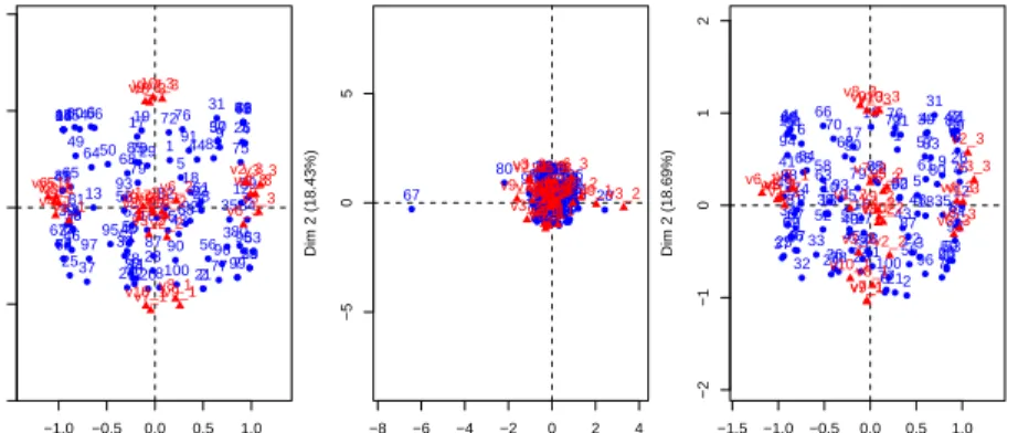
us consider an example to illustrate these problems with 100 individuals, 10 variables and a strong structure (the simulation process is detailed in the sim-ulation section). The two-dimensional configuration associated to this dataset is given figure 1 on the left. Then, 10% of values are removed and theiterative MCAalgorithm is performed on this incomplete dataset. The fitting error (cor-responding to the criterion (2)) and the error of prediction (using the matrix 1−Wrather thanWin the criterion (2)) are quite close (0.027 versus 0.057). The configuration obtained with the iterative MCA algorithm (not presented here) is very similar to the true one. Consequently, with 10% missing values there is no overfitting problem in this case. However, when more values are re-moved (leading for example to 30% missing values) the iterative MCA algorithm encounters difficulties. Indeed, with 30% missing values, the fitting error is low (0.024) whereas the prediction error is nearly 5 times higher (0.119), which is characteristic of the overfitting problem. Within the MCA configuration, the overfitting problem results in points (individuals and categories) that are very far from each other (see figure 1 in the middle). This is very frequent when datasets have many missing values. In the same way, overfitting is exacerbated with a low structure even if the percentage of missing values is small.
A first way to reduce overfitting is to reduce the number of dimensions for the imputation step in order to estimate less parameters; however it is important not to remove too many components since information can be lost. Another so-lution commonly used to overcome overfitting problems is to resort to shrinkage methods. Such methods have been mainly described in regression frameworks (Hastie et al., 2001). For example, the ridge estimator (Hoerl and Kennard, 1970) is slightly biased but has a smaller variance than the least square estima-tor. Consequently, the mean squared error of the parameters (squared bias plus variance) is often better with a ridge regression than with an ordinary regression. Further, a ridge regression gives better predictions. In the framework of MCA, the same principles apply: the estimation of the parameters (axes and compo-nents) and the prediction of the missing values obtained by theiterative MCA
algorithm may have a very high variance whereas a regularized version of this algorithm stabilizes these predictions. In the next section, such an algorithm is presented.
4.2
Regularized iterative MCA algorithm
The regularized algorithm is quite similar to the iterative MCA one but a “shrunk” reconstruction step is substituted to the classic reconstruction step (step 2.b). Withλsthe eigenvalue of ranks, step (2.b) can be rewritten as:
(ˆzikℓ −1) s Ikℓ−1 IJ = S X s=2 ˆ fℓ is kˆfℓ skD (pλs)ˆuℓks ! .
This step is then replaced by: (ˆzikℓ −1) s Ikℓ−1 IJ = S X s=2 ˆ fℓ is kˆfℓ skD p λs− ˆ σ2 √ λs ˆ uℓks ! , (4) withσ2
estimated by the mean of the last eigenvalues: ˆσ2
= 1 K−J−S
PK−J
s=S+1λs.
This new algorithm namedregularized iterative MCAis based on the algorithm proposed in Josse et al. (2009) and Ilin and Raiko (2010) to perform PCA on an incomplete dataset. The regularized term derives from a probabilistic formula-tion of PCA (Tipping and Bishop, 1999). The raformula-tionale of this algorithm is to remove the noise to avoid instability on the predictions. Implicitly, it is assumed that the first dimensions contain both information and noise whereas the last ones are restricted to noise. That is why the noise variance is estimated by the mean of the last eigenvalues. Each dimension is shrunk and the regularization term (in equation 4) is well-fitted since the smallest singular values are more shrunk than the firsts. In the extreme cases when there is no noise (σis equal to zero), theregularized iterative MCAalgorithm is equivalent to the iterative MCAalgorithm. At the opposite, when the noise is very important, the right hand term in equation (4) is close to 0, consequently, ˆzikis close to 1 and ˆxikis
close to Ik
I for alliandk. It corresponds to an imputation with the proportion
of each category. This behaviour is satisfactory since there is no information in the dataset. The regularization then remains to shrink the coordinates of the individuals towards the origin.
This new algorithm is thus a way to avoid overfitting. It can be illustrated by performing the algorithm on the examples of the overfitting section. When there is no overfitting problem (in the example with a strong structure and 10% missing values), the regularized algorithm gives roughly the same results than the non regularized version (the fitting error is within the same magnitude than the prediction error and the graphical outputs are quite similar). However, when the overfitting problem occurs (in the examples with a low structure or with a high percentage of missing values), the graphical outputs as well as the associ-ated errors are more convincing. More precisely, with the strong structure and 30% missing values, the fitting error and the prediction error are approximately of the same magnitude (0.026 versus 0.056) and there are no points distant from the centre of gravity in the MCA map (figure 1 on the right). The MCA map is very close to the true configuration (figure 1 on the left).
Remark 1. The regularized algorithm can be seen as a mix between a prin-cipal components regression and a ridge regression. Indeed, in the former, the last components (corresponding to the smallest eigenvalues) are omitted for the analysis whereas in the latter all the eigenvalues are shrunk with a larger amount of shrinkage for the last dimensions (Hastie et al., 2001). In theregularized
it-erative MCAalgorithm, there is a double shrinkage: the last components are
omitted and the subsequent eigenvalues are shrunk.
Remark 2. Takane and Hwang (2006) have proposed a regularized version of MCA for complete datasets to better estimate the parameters (in terms of
mean squared errors). They explain that regularization is all the more effective when MCA is performed on datasets with small to moderate sample size or on datasets containing categories with small frequencies. It reinforces the idea that the regularization is crucial for incomplete datasets. Indeed, when there are missing values in a dataset, this means less data and less information which can be seen as a particular case of datasets with small sample size.
5
Results
In this section, the main methods available to deal with missing data in MCA are assessed on a toy dataset, on simulations and on a real dataset.
5.1
A toy dataset
To illustrate the behaviour of theregularized iterative MCAas well as the other methods, we use a toy dataset with 9 individuals and 4 categorical variables
X, Y, Z, T (table 1). The first four individuals take the first category of the
var\ind 1 2 3 4 5 6 7 8 9
X Xa Xa Xa Xa Xb Xb Xb Xb Xb
Y Ya Ya Ya Ya Yb Yb Yc Yc Yc
Z Za Za Za Za Zb Zc Zb Zc Zc
T Ta Tb Ta Tb Ta Tb Ta Tb Ta
Table 1: Toy dataset (individuals are in columns).
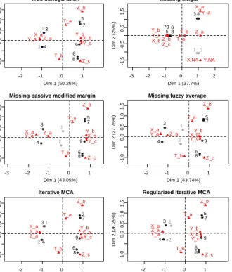
variables X, Y, and Z. The other individuals take other categories for these three variables and there is no link between these categories. The fourth vari-able T is very different from the others. The two dimensional configuration of the MCA obtained from this dataset is represented on the top left figure 2. Categories Xa, Ya and Za are superimposed as well as the individuals 2 and
4, respectively 1 and 3. Some elements are then removed for the individuals (1,2) for the variablesX andY (represented in grey in figure 2). Missing values are inserted on the categories which are highly linked to better spotlight the differences between methods.
Themissing single,missing passive modified margin,missing fuzzy average,
iterative MCA, and regularized iterative MCAmethods are performed. For the
two iterative MCA algorithms, one dimension has been used (in the imputation step) since the cross-validation algorithm on the incomplete dataset suggests one dimension. The two dimensional configuration obtained by the missing
singlemethod (top right) is very different from the configuration obtained with
the complete dataset. Indeed, the introduction of a new category (here NA for not available) for the missing values notably modifies the distances between individuals and generates a specific dimension (the second dimension).
The map obtained with themissing fuzzy averagemethod (middle left) shows that individuals 1 and 2 get closer to the centre of gravity. Indeed their missing values are imputed with the proportion and an individual in the indicator ma-trix which would have values equal to the proportion for each category would be at the centre of gravity on the MCA map. The map obtained with themissing
passive modified margin method (middle right) is quite similar to themissing
fuzzy averageone. Themissing passive modified margin method considers that
individuals with missing values for a categorical variable have not taken any available categories. Consequently, individual 1 for example only takes cate-goriesZa andTa and is at the barycentre of these two categories on the map.
The solution of theiterative MCAalgorithm is very close to the true config-uration. The rationale of the method is that the link between the categoriesXa, Ya andZa is learned with individuals 3 and 4; consequently since individuals 1
and 2 take the categoryZa, it is implicitly more plausible that they take the
categoriesXaandYa (the indicator matrix is then imputed with values close to
1). Theiterative MCAalgorithm provides a perfect fit. Since the links between variables are in that example perfect, the prediction is thus very good. How-ever, finding the best fit (minimizing the fitting error equation (2)) may lead to overfitting problems when the links between variables are not perfect or when there are many missing values. Indeed, the method believes in link even if it is artificial which may lead to bad predictions.
The configuration obtained with the regularized iterative MCA algorithm (bottom right) is between theiterative MCAone and themissing fuzzy average
one. This behaviour is expected because of the regularization term (equation (4)). Consequently, the method takes into account the links between categories (as the iterative MCA algorithm) but the regularization get the individuals slightly closer to the centre of gravity. In a way, the algorithm does not believe entirely in the links between variables which is often a good behaviour. The method balances between overfit (iterative MCA) and underfit (missing fuzzy
average).
In this example, the iterative MCA algorithm lead to better results than the regularized algorithm, but is is only because the relationship between variables are perfect. In all other situations the regularization algorithm is the best one.
5.2
Simulation studies
A simulation study was conducted to compare the missing single, themissing
passive modified margin, themissing fuzzy average and theregularized iterative
MCAmethods. The performances of these methods are assessed from different simulated datasets with varying parameters: the percentage of missing values (small and medium), the kind of missing values (MCAR and MAR), the pattern of missing values either random or non-random (for non-random, some individ-uals do not answer to a set of questions), the relationships between variables (low and strong). For each set of parameters, 1000 simulations are drawn.
The RV coefficient (Escoufier, 1973; Josse et al., 2008) is used to assess the performances of the different methods. The RV coefficient is a correlation
coefficient between two matrices which allows to compare the relative positions of the objects from one configuration to another. A modified version of the RV coefficient has been proposed (Smilde et al., 2009) in order to better interpret this coefficient. Indeed under the null hypothesis of independence between the two configurations, the expectation of the RV coefficient is not equal to 0 and depends on the number of rows and on the structure of the dataset. The modified RV coefficient eliminates this effect and its expectation is equal to 0 when there is no relationship between the two data tables.
5.2.1 Protocol of simulation
More precisely, the datasets are built using the following procedure:
• A dataset with 100 individuals and 10 variables is drawn from a multi-variate normal distribution with a two-block diagonal covariance matrix; one block has size 6×6 and the other 4×4. The same level of correlation is used for each block, 0.4 for the low structure and 0.8 for the strong structure.
• Each variable is distributed in three equal-count categories.
• MCAR case: 10% and 30% missing values are inserted either at random (it corresponds to the random pattern) or in the following way (corre-sponding to the non-random pattern): there are missing values for the first 60 individuals on the first 3 variables and for the last 60 individuals on variables 9 and 10. For both pattern, such missing values are MCAR because they do not depend on any values (missing or not).
• MAR case: missing values are inserted in variables 2 to 6 when the variable 1 takes the first category and for variables 8 to 10 when the variable 7 takes the last category. 8% or 16% missing values are inserted either with a random pattern or not.
The number of underlying dimensions of the simulated dataset is by construction equal to four (since there are two independent blocks of variables and three categories per variable,i.e. two dimensions for each block). The cross-validation algorithm also suggests four dimensions.
5.2.2 Behaviour of the iterative algorithms
First, let us assess the behaviour of the two iterative algorithms namely the
iter-ative MCA(denoted iMCA) algorithm as well as theregularized iterative MCA
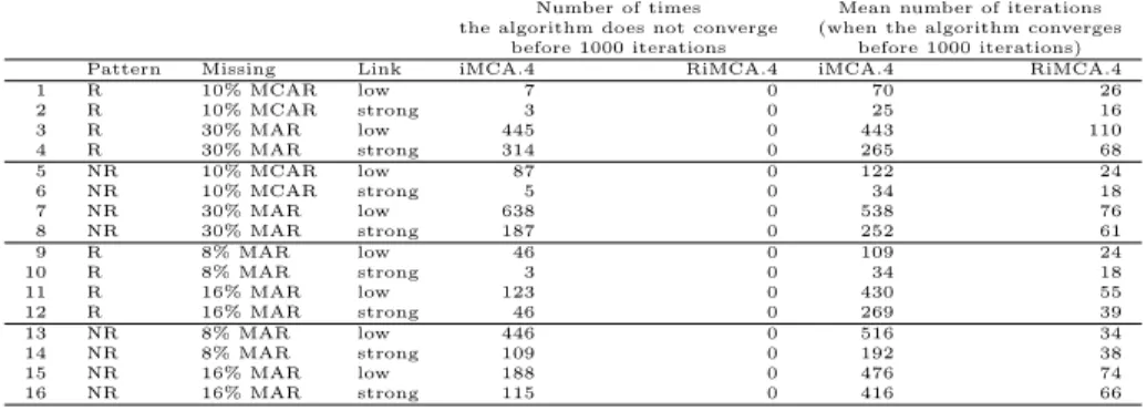
(denoted RiMCA) algorithm. Table 2 presents, within the first two columns, the number of times (over 1000 simulations) that the algorithms do not reach a solution before 1000 iterations. The regularized iterative MCA always reaches a minimum before 1000 iterations whereas the iterative MCA algorithm en-counters difficulties. In these cases, the number of iterations varies between 1000 and 25000. Such situations correspond to overfitted solutions where some
points (individuals or categories) are more distant from the centre of gravity as illustrated in figure 1.
Table 2: Convergence properties of the algorithms iMCA and RiMCA Number of times Mean number of iterations the algorithm does not converge (when the algorithm converges
before 1000 iterations before 1000 iterations) Pattern Missing Link iMCA.4 RiMCA.4 iMCA.4 RiMCA.4
1 R 10% MCAR low 7 0 70 26 2 R 10% MCAR strong 3 0 25 16 3 R 30% MAR low 445 0 443 110 4 R 30% MAR strong 314 0 265 68 5 NR 10% MCAR low 87 0 122 24 6 NR 10% MCAR strong 5 0 34 18 7 NR 30% MAR low 638 0 538 76 8 NR 30% MAR strong 187 0 252 61 9 R 8% MAR low 46 0 109 24 10 R 8% MAR strong 3 0 34 18 11 R 16% MAR low 123 0 430 55 12 R 16% MAR strong 46 0 269 39 13 NR 8% MAR low 446 0 516 34 14 NR 8% MAR strong 109 0 192 38 15 NR 16% MAR low 188 0 476 74 16 NR 16% MAR strong 115 0 416 66
The last two columns of this table give the means of the number of iterations when the algorithms have converged in less than 1000 iterations. This highlights the fact that the regularized algorithm is always the fastest.
The iterative MCA algorithm encounters many problems, is very slow to
converge and often converges to overfitted solutions. Consequently the results of this method are not presented hereafter.
5.2.3 Results of the simulations
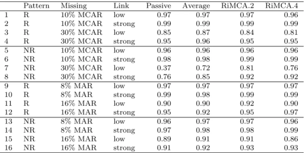
Table 3 (resp. table 4) gives the results for the configuration of the individuals (resp. categories). For each set of parameters, the modified RV coefficient is computed between the initial two-dimensional configuration (without missing values) and the two-dimensional configurations obtained by each method. The median over the 1000 modified RV coefficients is retained. The letter R corre-sponds to the random pattern of missing values whereas NR correcorre-sponds to the non-random pattern of missing values. For the missing single method (NA), there are only the results for individuals.
The boxplots of two particular sets of parameters with important differences between the medians (rows 8 and 12 of table 3) are given figure 3. We observe that in these two cases (30% MCAR, strong structure, random pattern and 16% MAR, strong structure, random pattern) the variability of the results for the different methods are quite small and very similar. This remark remains true for the other rows of table 3. Consequently the medians in table 3 can be safely interpreted.
Concerning the individuals (table 3), the performances of themissing single
method (NA) are very poor for each parameter set and especially for non-random patterns (NR) since distances between individuals are highly affected.
For all the other methods, the results are satisfying for a small percentage of missing values. As expected, the performances decrease when the percentage
Pattern Missing Link Passive Average NA RiMCA.2 RiMCA.4 1 R 10% MCAR low 0.94 0.94 0.87 0.94 0.94 2 R 10% MCAR strong 0.97 0.97 0.96 0.98 0.98 3 R 30% MCAR low 0.76 0.76 0.67 0.76 0.72 4 R 30% MCAR strong 0.88 0.88 0.86 0.91 0.92 5 NR 10% MCAR low 0.91 0.92 0.46 0.93 0.92 6 NR 10% MCAR strong 0.94 0.95 0.67 0.97 0.98 7 NR 30% MCAR low 0.43 0.77 0.30 0.78 0.73 8 NR 30% MCAR strong 0.71 0.91 0.45 0.90 0.90 9 R 8% MAR low 0.94 0.94 0.72 0.95 0.95 10 R 8% MAR strong 0.96 0.96 0.96 0.98 0.99 11 R 16% MAR low 0.86 0.82 0.50 0.87 0.85 12 R 16% MAR strong 0.88 0.84 0.88 0.94 0.96 13 NR 8% MAR low 0.91 0.90 0.28 0.92 0.92 14 NR 8% MAR strong 0.91 0.90 0.54 0.96 0.97 15 NR 16% MAR low 0.80 0.79 0.28 0.83 0.79 16 NR 16% MAR strong 0.79 0.77 0.54 0.89 0.91
Table 3: Median over 1000 replications of the modified RV coefficient between the true configuration of individuals and the configurations of individuals ob-tained with each method; Passive formissing passive modified margin, Average for themissing fuzzy average, NA formissing single and RiMCA for the
regu-larized iterative MCAmethods with 2, and 4 dimensions; R for random pattern
and NR for non-random.
Pattern Missing Link Passive Average RiMCA.2 RiMCA.4
1 R 10% MCAR low 0.97 0.97 0.97 0.96 2 R 10% MCAR strong 0.99 0.99 0.99 0.99 3 R 30% MCAR low 0.85 0.87 0.84 0.81 4 R 30% MCAR strong 0.95 0.96 0.95 0.95 5 NR 10% MCAR low 0.96 0.96 0.96 0.96 6 NR 10% MCAR strong 0.98 0.98 0.99 0.99 7 NR 30% MCAR low 0.37 0.72 0.81 0.76 8 NR 30% MCAR strong 0.76 0.85 0.92 0.92 9 R 8% MAR low 0.97 0.97 0.97 0.97 10 R 8% MAR strong 0.99 0.98 0.99 0.99 11 R 16% MAR low 0.90 0.90 0.92 0.90 12 R 16% MAR strong 0.95 0.92 0.95 0.97 13 NR 8% MAR low 0.96 0.97 0.97 0.96 14 NR 8% MAR strong 0.97 0.98 0.98 0.99 15 NR 16% MAR low 0.89 0.91 0.91 0.86 16 NR 16% MAR strong 0.91 0.92 0.93 0.93
Table 4: Median over 1000 replications of the modified RV coefficient between the true categories configuration and the configurations of individuals obtained with each method; Passive formissing passive modified margin, Average for the
missing fuzzy averageand RiMCA for theregularized iterative MCAwith 2, and
4 dimensions; R for random pattern and NR for non-random. of missing values increases.
(Pas-sive) and themissing fuzzy average method (Average) are quite similar in most situations. One can remark that in MAR situation, themissing fuzzy average
method (Average) gives very poor results. This behaviour is expected because
it doesn’t take into account the relationships between the variables in the im-putation.
The regularized iterative MCA method with four dimensions RiMCA.4 is
the most stable across the different patterns of missing values and the different percentages of missing values. The regularized method always provides good results even if in 4 cases it doesn’t give the best ones. The other methods provide good results in many situations (except thesingle missing method which is not well fitted for such missing data) but sometimes they can really crash. That is a strong argument in favour of theregularized iterative MCAmethod. The four situations (rows 3, 7, 11, and 15) when the algorithm does not provide the best results can be explained as follows. It corresponds to situations where the link is low and the percentage of missing values is important. In these four cases
theregularized iterative MCAmethod with two dimensions RiMCA.2 takes the
lead. This behaviour may be explained since with low structures and many missing values, the instability increases with the number of dimensions. The estimation of the individual configurations is then better with two dimensions than with four dimensions. This behaviour is understandable. Indeed, in such situations the underlying four-dimensional structure is too low and may have disappeared. The last dimensions are not sufficiently strong and are not very stable. Consequently, taking less dimensions is a way to stabilize the predictions. From a practical point of view, the number of underlying dimensions is unknown and when the data contains many missing values and a low structure, taking few dimensions in the RiMCA algorithm should be preferred by the user. The results obtained for the categories (table 4) are quite similar to the results obtained for the individuals.
5.3
Real data analysis
A user satisfaction survey of pleasure craft operators on the “Canal des Deux Mers”, located in South of France, was carried out by the public corpora-tion “Voies Navigables de France” responsible for managing and developing the largest network of navigable waterways in Europe. Pleasure craft operators were asked their opinion about numerous questions with categorical answers, each item having two or three categories of response. 1232 individuals answered 14 questions with a total of 35 categories. There is 9% missing values in this dataset which concerns 42% of respondents. The data are available in the R
packagemissMDA(Husson and Josse, 2010).
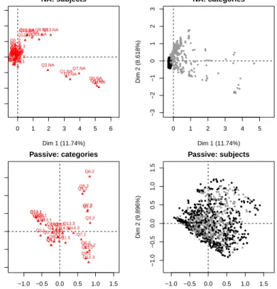
Figure 4 gives the two-dimensional maps of the categories and of the indi-viduals obtained by the missing single (NA) method and the missing passive
modified margin(Passive) one. The plot of the categories for themissing single
(NA) method (figure 4, top left) is dominated by the missing categories (denoted for instance Q2 NA, for the non-response to question 2). The pattern of missing values,i.e. the associations between non-responses to certain questions, can be
visualized (for instance non-response to ’Q4’ is associated to non-response to ’Q5’ and ’Q6’). Such pattern frequently arises in questionnaires when individu-als do not answer to set of items. These missing values can be MAR, MCAR or MNAR because they can depend on other variables and it does not affect the kind of missing values. For example, missing values are MCAR if some respon-dents have skipped the last items in the questionnaire due to time constraints. However, it may also represent a particular behaviour and a sub-population of respondents.
The plot of the categories for the missing passive modified margin (Passive) method (figure 4, bottom left) “skips” the missing values and avoids the draw-back of the NA method where the first dimensions are dominated by the missing values.
Figure 5 gives the plots of the categories and the individuals in the plane 1-2 obtained with the iterative MCA and the regularized iterative MCA methods. The plot of the individuals for the iterative MCA method (figure 5, bottom right) highlights the overfitting problem already presented in section 4.1 (some individuals are distant from the others). The plot of the individuals for the
regularized iterative MCAmethod (figure 5, top right) confirms the importance
of the regularization to reduce this phenomenon.
Note that in this real data example, the results obtained with themissing
passive modified margin(Passive) and theiterative MCAmethods are very
sim-ilar. This is not in contradiction with the results of the simulations where the performances of the two methods were very similar in many situations especially with small percentage of missing values.
6
Discussion
This paper proposes theregularized iterative MCAalgorithm to handle missing values in MCA which is a major issue especially when dealing with question-naires. The proposed algorithm is a regularized version of an EM-type algorithm where missing values are filled in with the expected values (via the reconstruc-tion formulae of orderS) in the expectation step and the axes and components are obtained during the maximization step. The regularization is crucial because it limits the overfitting problem. When missing values mask underlying values among the available categories and are MAR or MCAR, regularized iterative MCAgives slightly better results than the other methods. This is particularly true for MAR values and when data are structured,i.e. when there are strong relationships between variables. However, this method has some drawbacks: convergence problems may occur due to the iterative nature of the algorithm and it is necessary to choose a tuning parameter (the number of components). This number is chosen by a cross-validation algorithm.
Theregularized iterative MCAis implemented in the R package (R
Develop-ment Core Team, 2010)missMDA(Husson and Josse, 2010). To perform MCA with missing values two steps are required. First, the functionimputeMCA per-forms the regularized algorithm and gives as an output a completed indicator
matrix. Then this completed indicator matrix is used as an input of the multi-ple correspondence analysis functionMCAof theFactoMineRpackage (?Husson et al., 2011) to obtain the classical outputs of MCA (graphs, scores, loadings.)
MCA is sometimes used as a preprocessing step before clustering methods. If
themissing singlemethod is used, it may lead to distances between individuals
disturbed by the missing entries. The regularized iterative MCA is well-fitted since its main objective is to predict the coordinates of the individuals on the first components in spite of the missing values. This strategy is then a way to perform clustering on incomplete categorical variables.
It may be interesting to assess the performances of the regularized
itera-tive MCAalgorithm as an imputation algorithm and to compare it to several
approaches dealing with nonresponses in categorical variables. A model often used for imputation of categorical variables is the log-linear model (Schafer, 1997). However, the log-linear model can only be used for a small number of variables since it requires to compute all the entries of the multi-way cross ta-ble. Other procedures have been proposed especially in the context of the item response theory (IRT) but they are mainly devoted to dichotomous and ordi-nal data rather than to categorical ones. Recently, Vermunt et al. (2008) have proposed the use of the latent class model to impute large datasets. The
regu-larized iterative MCAalgorithm might be competitive since it can be applied on
large datasets and uses both similarities between individuals and relationships between variables for the imputation.
References
J-P. Benz´ecri. L’analyse des donn´ees. Tome II: L’analyse des correspondances. Dunod, 1973.
R. Bro, K. Kjeldahl, A. K. Smilde, and H. A. L. Kiers. Cross-validation of component model: a critical look at current methods. Anal Bioanal Chem, 390:1241–1251, 2008.
J de Leeuw and P G M van der Heijden. Correspondence analysis of incomplete contingency tables. Psychometrika, 53:223–233, 1988.
A P. Dempster, N M. Laird, and D B. Rubin. Maximum likelihood from incom-plete data via the em algorithm. Journal of the Royal Statistical Society B, 39:1–38, 1977.
B. Escofier. Traitement des questionnaires avec non r´eponse, analyse des corre-spondances avec marges modifi´ee et analyse multicanonique avec contrainte.
Publications de l’institut de statistique de l’universit´e de Paris, 32:33–70,
1987.
Yves Escoufier. Le traitement des variables vectorielles.Biometrics, 29:751–760, 1973.
K.R. Gabriel and S. Zamir. Lower rank approximation of matrices by least squares with any choice of weights. Technometrics, 21:236–246, 1979. A. Gifi. Non-linear Multivariate Analysis. D.S.W.O.-Press, Leiden, 1981. Michael Greenacre. Theory and Applications of Correspondence Analysis.
Acadamic Press, 1984.
Michael Greenacre. Correspondence analysis of multivariate categorical data by weighted least-squares. Biometrika, 75:457–477, 1988.
Michael Greenacre and J Blasius.Multiple Correspondence Analysis and Related
Methods. Chapman & Hall/CRC, 2006.
Michael Greenacre and R. Pardo. Subset correspondence analysis: visualizing relationships among a selected set of response categories from a questionnaire survey. Sociological methods and research, 35 (2):193–218, 2006.
T Hastie, R Tibshirani, and J Friedman. The elements of statistical learning.
Data Mining, Inference and Prediction. Springer series in statistics, 2001.
A F Hoerl and R W Kennard. Ridge regression: Biased estimation for nonorthogonal problems. Technometrics, 12:55–67, 1970.
Francois Husson and Julie Josse. missMDA: Handling missing
val-ues with/in multivariate data analysis (principal component
meth-ods), 2010. URL http://www.agrocampus-ouest.fr/math/husson, http://www.agrocampus-ouest.fr/math/josse. R package version 1.2. Francois Husson, Julie Josse, Sebastien Le, and Jeremy Mazet. FactoMineR:
Multivariate Exploratory Data Analysis and Data Mining with R, 2011. URL
http://factominer.free.fr, http://www.agrocampus-ouest.fr/math/. R package version 1.16.
A Ilin and T. Raiko. Practical approaches to principal component analysis in the presence of missing values. Journal of Machine Learning Research, page To appear, 2010.
J Josse, J Pag`es, and F Husson. Testing the significance of the rv coefficient.
Computational Statistics and Data Analysis, 53:82–91, 2008.
J Josse, J Pag`es, and F Husson. Gestion des donn´ees manquantes en analyse en composantes principales. Journal de la Soci´et´e Fran¸caise de Statistique, 150: 28–51, 2009.
H A L Kiers. Weighted least squares fitting using ordinary least squares algo-rithms. Psychometrika, 62:251–266, 1997.
L Lebart, A Morineau, and K M Werwick. Multivariate Descriptive Statistical
R J A Little and D B Rubin. Statistical Analysis with Missing Data. Wiley series in probability and statistics, New-York, 1987, 2002.
J Meulman.Homgeneity Analysis of Incomplete Data. D.S.W.O.-Press, Leiden, 1982.
G Michailidis and J de Leeuw. The gifi system of descriptive multivariate anal-ysis. Statistical Science, 13:307–336, 1998.
S Nishisato. Analysis of Categorical Data: Dual Scaling and its Applications. University of Toronto Press, Toronto, 1980.
C Nora-Chouteau. Une m´ethode de reconstitution et d’analyse de donn´ees
in-compl`etes. PhD thesis, Universit´e Pierre et Marie Curie, 1974.
R Development Core Team. R: A Language and Environment for Statistical
Computing. R Foundation for Statistical Computing, Vienna, Austria, 2010.
URLhttp://www.R-project.org/. ISBN 3-900051-07-0.
D B Rubin. Inference and missing data. Biometrika, 63:581–592, 1976. J L Schafer. Analysis of Incomplete Multivariate Data. Chapman & Hall/CRC,
1997.
J L Schafer and J W Graham. Missing data: Our view of the state of the art.
Psychological Methods, 7:147–177, 2002.
A K Smilde, H A L Kiers, S Bijlsma, C M Rubingh, and M J van Erk. Matrix correlations for high-dimensional data: the modified RV-coefficient.
Bioinfor-matics, 25:401–405, 2009.
Y Takane and H Hwang. Generalized constrained canonical correlation analysis.
Multivariate Behavioral Research, 37:163–195, 2002.
Y Takane and H Hwang. Regularized multiple correspondence analysis. In J Blasius and M J Greenacre, editors,Multiple Correspondence Analysis and
Related Methods, pages 259–279. Chapman & Hall, 2006.
Y Takane and Y Oshima-Takane. Relationships between two methods for dealing with missing data in principal component analysis.Behaviormetrika, 30:145– 154, 2003.
M Tenenhaus and F W Young. An analysis and synthesis of multiple corre-spondence analysis, optimal scaling, dual scaling, homogeneity analysis and other methods for quantifying categorical multivariate data. Psychometrika, 50:91–119, 1985.
M Tipping and C M Bishop. Probabilistic principal component analysis.Journal
P.G.M. van der Heijden and B Escofier. Multiple correspondence analysis with missing data. InAnalyse des correspondances. Presse universitaire de Rennes, 2003.
J K Vermunt, J R van Ginkel, L A van der Ark, and K Sijtsma. Multiple impu-tation of incomplete categorical data using latent class analysis. Sociological
−1.0 −0.5 0.0 0.5 1.0 −2 −1 0 1 2 True configuration Dim 1 (21.28%) Dim 2 (15.88%) 1 2 3 4 5 6 7 8 9 10 11 12 13 14 15 16 17 18 19 20 21 22 23 24 25 26 27 28 29 30 31 32 33 34 35 36 37 38 39 40 41 42 43 44 45 46 47 48 49 50 51 52 53 54 55 56 57 58 59 60 61 62 63 64 65 66 67 68 69 70 71 72 73 74 75 76 77 78 79 80 81 82 83 84 85 86 87 88 89 90 91 92 93 94 95 96 97 98 99 100 v1_1 v1_2 v1_3 v2_1 v2_2 v2_3 v3_1 v3_2 v3_3 v4_1 v4_2 v4_3 v5_1 v5_2 v5_3 v6_1 v6_2 v6_3 v7_1 v7_2 v7_3 v8_1 v8_2 v8_3 v9_1 v9_2 v9_3 v10_1 v10_2 v10_3 −8 −6 −4 −2 0 2 4 −5 0 5
Iterative MCA configuration
Dim 1 (32.91%) Dim 2 (18.43%) 1 23 4 5 6 7 8 9 1011 12 13 1415 1617 18 192221 20 23 24 25 26 272829 3031 32 33 34 35 36 37 38 39 40 41 42 43 44 45 46 47 48 49 50 51 52 53 54 5556 57 58 59 60 61 62 63646566 67 68 69 70 71 72 7374 75 76 77 78 79 80 81 82 8384 85 86 87 88 89 9091 92 93 94 95 96 97 9899 100 v1_1 v1_2 v1_3 v2_1 v2_2 v2_3 v3_1 v3_2 v3_3 v4_1 v4_2 v4_3 v5_1 v5_2v5_3 v6_1 v6_2 v6_3 v7_1 v7_2v8_2v7_3v8_1 v8_3 v9_1 v9_2 v9_3v10_3v10_1v10_2 −1.5 −1.0 −0.5 0.0 0.5 1.0 −2 −1 0 1 2
Regularized iterative MCA configuration
Dim 1 (25.11%) Dim 2 (18.69%) 1 2 3 4 5 6 7 8 9 10 11 12 13 14 15 16 17 18 19 20 21 22 23 24 25 26 27 28 29 30 31 32 33 34 35 36 37 38 39 40 41 42 43 44 45 46 47 48 49 50 51 52 53 54 55 56 57 58 59 60 61 62 63 64 65 66 67 68 69 70 72 71 7374 75 76 77 78 79 80 81 82 83 84 85 86 87 88 89 90 91 92 93 94 95 96 97 98 99 100 v1_1 v1_2 v1_3 v2_1 v2_2 v2_3 v3_1 v3_2 v3_3 v4_1 v4_2 v4_3 v5_1 v5_2 v5_3 v6_1 v6_2 v6_3 v7_1 v7_2 v7_3 v8_1 v8_2 v8_3 v9_1 v9_2 v9_3 v10_1 v10_2 v10_3
Figure 1: Illustration of the overfitting problem on the MCA map obtained on a dataset with a strong structure and 30% missing values. The true configuration is on the left, the configuration obtained with theiterative MCA algorithm is in the middle, the configuration obtained with the regularized iterative MCA
2 -2 -1 0 1 -1 .0 0 .0 0 .5 1 .0 1 .5 True configuration Dim 1 (50.26%) D im 2 ( 2 4 .7 1 % ) 1 2 3 4 5 6 7 8 9 X_a X_b Y_a Y_b Y_c Z_a Z_b Z_c T_a T_b -3 -2 -1 0 1 2 -1 .5 -0 .5 0 .5 1 .5 Missing single Dim 1 (37.7%) D im 2 ( 2 5 % ) 1 2 3 4 56 7 8 9 X.NA X_a X_b Y.NA Y_a Y_b Y_c Z_a Z_b Z_c T_a T_b -3 -2 -1 0 1 -1 .0 0 .0 0 .5 1 .0 1 .5
Missing passive modified margin
Dim 1 (43.05%) D im 2 ( 2 3 .0 3 % ) 1 2 3 4 5 6 7 8 9 X_a X_b Y_a Y_b Y_c Z_a Z_b Z_c T_a T_b -2 -1 0 1 -1 .0 0 .0 0 .5 1 .0 1 .5
Missing fuzzy average
Dim 1 (43.74%) D im 2 ( 2 7 .7 5 % ) 1 2 3 4 5 6 7 8 9 X_a X_b Y_a Y_b Y_c Z_a Z_b Z_c T_a T_b -2 -1 0 1 -1 .0 0 .0 0 .5 1 .0 1 .5 Iterative MCA Dim 1 (50.35%) D im 2 ( 2 4 .7 5 % ) 1 3 4 5 6 7 8 9 X_a X_b Y_a Y_b Y_c Z_a Z_b Z_c T_a T_b -2 -1 0 1 -1 .0 0 .0 0 .5 1 .0 1 .5
Regularized iterative MCA
Dim 1 (48.17%) D im 2 ( 2 6 .2 9 % ) 1 2 3 4 5 6 7 8 9 X_a X_b Y_a Y_b Y_c Z_a Z_b Z_c T_a T_b
Figure 2: Comparison of themissing single, missing passive modified margin,
missing fuzzy average, iterative MCA, and regularized iterative MCA methods
Passive Average NA RiMCA.2 RiMCA.4 0.0 0.2 0.4 0.6 0.8 1.0
30 % MCAR ; link= strong ; pattern= non−random individual configuration
Passive Average NA RiMCA.2 RiMCA.4
0.0 0.2 0.4 0.6 0.8 1.0
16 % MAR ; link= strong ; pattern= random individual configuration
Figure 3: Boxplots of the modified RV coefficients over the 1000 simulations for the case NR, 30% MCAR, strong, R (left) and 16% MAR, strong, R (right)
0 1 2 3 4 5 6 −3 −2 −1 0 1 2 3 NA: subjects Dim 1 (11.74%) Dim 2 (8.618%) Q1.NA Q1_1 Q1_2Q1_3 Q2.NA Q2_1 Q2_2Q2_3 Q3.NA Q3_1 Q3_2Q3_3 Q4.NA Q4_1 Q4_2 Q5.NA Q5_1 Q5_2 Q6.NA Q6_1 Q6_2 Q7.NA Q7_1Q7_2 Q8.NA Q8_1Q8_2 Q9.NA Q9_1 Q9_2 Q9_3 Q10.NA Q10_1 Q10_2 Q11.NA Q11_1 Q11_2 Q12.NA Q12_1 Q12_2Q12_3 Q13.NA Q13_1 Q13_2Q13_3 Q14.NA Q14_1 Q14_2Q14_3 0 1 2 3 4 5 −3 −2 −1 0 1 2 3 NA: categories Dim 1 (11.74%) Dim 2 (8.618%) −1.0 −0.5 0.0 0.5 1.0 1.5 −1.0 −0.5 0.0 0.5 1.0 1.5 Passive: categories Dim 1 (12.72%) Dim 2 (9.896%) Q1.1 Q1.2 Q1.3 Q2.1 Q2.2 Q2.3 Q3.1 Q3.2 Q3.3 Q4.1 Q4.2 Q5.1 Q5.2 Q6.1 Q6.2 Q7.1 Q7.2 Q8.1 Q8.2 Q9.1 Q9.2 Q9.3 Q10.1 Q10.2 Q11.1 Q11.2 Q12.1 Q12.2 Q12.3 Q13.1 Q13.2 Q13.3 Q14.1 Q14.2Q14.3 −1.0 −0.5 0.0 0.5 1.0 1.5 −1.0 −0.5 0.0 0.5 1.0 1.5 Passive: subjects Dim 1 (12.72%) Dim 2 (9.896%)
Figure 4: Plot of the categories (left) and the individuals (right) in the principal plane 1-2 obtained by the missing single(NA) method (top) and obtained by
-1.0 -0.5 0.0 0.5 1.0 1.5 -0 .5 0 .0 0 .5 1 .0 1 .5
Regularized iterative MCA: categories
Dim 1 (14.58%) D im 2 ( 1 1 .2 1 % ) Q1.1 Q1.2 Q1.3 Q2.1 Q2.2 Q2.3 Q3.1 Q3.2 Q3.3 Q4.1 Q4.2 Q5.1 Q5.2 Q6.1 Q6.2 Q7.1 Q7.2 Q8.1 Q8.2 Q9.1 Q9.2 Q9.3 Q10.1 Q10.2 Q11.1 Q11.2 Q12.1 Q12.2 Q12.3 Q13.1 Q13.2 Q13.3 Q14.1 Q14.2Q14.3 -1.0 -0.5 0.0 0.5 1.0 1.5 -1 .0 -0 .5 0 .0 0 .5 1 .0 1 .5
Regularized iterative MCA: subjects
Dim 1 (14.58%) D im 2 ( 1 1 .2 1 % ) -0.5 0.0 0.5 1.0 1.5 2.0 -1 .5 -1 .0 -0 .5 0 .0 0 .5 1 .0 1 .5
iterative MCA: categories
Dim 1 (16.4%) D im 2 ( 1 5 .4 4 % ) Q1.1 Q1.2 Q1.3 Q2.1 Q2.2 Q2.3 Q3.1 Q3.2 Q3.3 Q4.1 Q4.2 Q5.1 Q5.2 Q6.1 Q6.2 Q7.1 Q7.2 Q8.1 Q8.2 Q9.1 Q9.2 Q9.3 Q10.1 Q10.2 Q11.1 Q11.2 Q12.1 Q12.2 Q12.3 Q13.1 Q13.2 Q13.3 Q14.1 Q14.2 Q14.3 -5 -4 -3 -2 -1 0 1 2 -5 -4 -3 -2 -1 0 1 2
iterative MCA: subjects
Dim 1 (16.4%) D im 2 ( 1 5 .4 4 % )
Figure 5: Plot of the categories (left) and the individuals (right) in the princi-pal plane 1-2 obtained by theregularized iterative MCAmethod (top) and the