Global Solar Radiation Estimation and Climatic
Variability Analysis Using Extreme Learning
Machine Based Predictive Model
TAO HAI 1, AHMAD SHARAFATI 2, ACHITE MOHAMMED 3, SINAN Q. SALIH 4,5,
RAVINESH C. DEO 6, NADHIR AL-ANSARI 7, AND ZAHER MUNDHER YASEEN 8
1Computer Science Department, Baoji University of Arts and Sciences, Baoji, China
2Department of Civil Engineering, Science and Research Branch, Islamic Azad University, Tehran, Iran
3Faculty of Nature and Life Sciences, Laboratory of Water and Environment, University Hassiba Benbouali Chlef, Hay Es-Salem Chlef, Algeria 4Institute of Research and Development, Duy Tan University, Da Nang 550000, Vietnam
5Computer Science Department, College of Computer Science and Information Technology, University of Anbar, Ramadi, Iraq
6School of Agricultural, Computational and Environmental Sciences, Centre for Applied Climate Sciences, Institute of Life Sciences and Environment, University of Southern Queensland, Springfield, QLD 4300, Australia
7Civil, Environmental and Natural Resources Engineering, Luleå University of Technology, 97187 Luleå, Sweden
8Sustainable Developments in Civil Engineering Research Group, Faculty of Civil Engineering, Ton Duc Thang University, Ho Chi Minh City, Vietnam
Corresponding author: Zaher Mundher Yaseen ([email protected])
ABSTRACT Sustainable utilization of the freely available solar radiation as renewable energy source requires accurate predictive models to quantitatively evaluate future energy potentials. In this research, an evaluation of the preciseness of extreme learning machine (ELM) model as a fast and efficient framework for estimating global incident solar radiation (G) is undertaken. Daily meteorological datasets suitable for G estimation belongs to the northern parts of the Cheliff Basin in Northwest Algeria, is used to construct the estimation model. Cross-correlation functions are applied between the inputs and the target variable (i.e., G) where several climatological information’s are used as the predictors for surface level G estimation. The most significant model inputs are determined in accordance with highest cross-correlations considering the covariance of the predictors with the G dataset. Subsequently, seven ELM models with unique neuronal architectures in terms of their input-hidden-output neurons are developed with appropriate input combinations. The prescribed ELM model’s estimation performance over the testing phase is evaluated against multiple linear regressions (MLR), autoregressive integrated moving average (ARIMA) models and several well-established literature studies. This is done in accordance with several statistical score metrics. In quantitative terms, the root mean square error (RMSE) and mean absolute error (MAE) are dramatically lower for the optimal ELM model with RMSE and MAE=3.28 and 2.32 Wm−2 compared to 4.24 and 3.24 Wm−2(MLR) and 8.33 and 5.37 Wm−2(ARIMA).
INDEX TERMS Energy feasibility studies, extreme learning machine, solar energy estimation, multivariate modeling, solar energy mapping.
I. INTRODUCTION
The growth in electrical energy demand is a becoming crit-ical issue especially, in promoting sufficient technologies for solar (and other renewable) energy utilization that must support United Nations Sustainable Development Goal 7 [1]. Meaningful improvements in the current energy usage will require a higher level of financing and bolder climate-energy policy commitments. In addition, the willingness of different The associate editor coordinating the review of this manuscript and approving it for publication was Long Wang .
countries to embrace new energy technologies including remote and regional mapping of energy prospectively on a much wider scale than currently available. Recent data suggests that there been a modest improvement in the pro-portion of renewable energy usage (from 17.9 per cent to 18.3 percent) and much of this increase has been the elec-tricity derived from water, solar and wind. The goal lies in the challenge of increasing the share of renewable energy in heat-ing and transport sectors that nominally account for 80 per cent of the global energy consumption (UNDP Goal 7) [1]. Considering this need, solar radiation energy can be used as This work is licensed under a Creative Commons Attribution 4.0 License. For more information, see http://creativecommons.org/licenses/by/4.0/
a renewable, reliable and economically viable energy com-pared to the other sources such as fossil fuels since solar energy extraction has a negligible impact on air pollution and other societal and human impact issues [2], [3]. In the last few decades, G has been widely investigated worldwide, driven by the rising price of oil, global warming issues and the growing of electrical energy demand due to industrialization and expansion of thriving economies [4]. G is received in the form of usable energy that originally exists in sunlight. This type of energy can be converted into: (i) electricity using photovoltaic, (ii) thermal energy where it can be uti-lized for water heating and (iii) chemical energy by photo-electrochemical tools for generating solar fuels [5]. All of these forms of energy require adequately mapped resources in regions where they are in abundance. However, to attain this goal, governments and energy companies need to firstly evaluate the availability of solar energy in remote, regional as well as in metropolitan regions.
To support future energy mapping, the estimation of solar radiation is therefore a crucial issue for solar energy furnaces, climate change simulations for different regions, and the design of solar powered plants [6], [7]. In addition, solar radi-ation can be employed to generate electricity, but this resource is an unsteady resource given the dependence on a range of local and regional climatic factors that act to moderate the availability of energy at the terrestrial land surface. To over-come any potential energy crisis issues brought about by the unstable and stochastic behavior of incident solar radiation, an accurate estimation of G (that can provide an indication of its current and the future availability) is essential, mainly to guide stakeholders in practical decisions made by energy operators to reach a balance between the stability of the supply, energy extraction efficiencies and the consumption of available electricity by various end-users [8].
Solar energy studies generally utilize two main approaches that are used to estimate and/or predict the G, namely the traditional (statistical or mathematical) and the soft comput-ing (SC) models [9]. The traditional approaches can be cat-egorized into the dynamic [10]–[12] and empirical [13]–[19] modeling phases. Dynamic methods are employed to predict the G in long term durations and over the global scale. These methods can be used to assess the long-term availability of energy; for example, in different seasons and over cli-matic anomalies and cycles such as the El Nino Southern Oscillation phases. There are many sources of uncertainty in the G predictions using empirical models, for instance, the need for initial conditions data that are largely site specific and also present a major difficulty in adequately mapping the solar energy in diverse regional and remote locations where it is generally hard to set up the measurement appa-ratus. Therefore, traditional methods may not be adequate and reliable to predict G in any given temporal and spatial scales, and especially, in both the short term and local scale. In recent decades, SC methods which do not require complex
mathematical equations or initial conditions data, have been introduced for predicting G using a range of covariates.
SC methods such as the artificial neural networks (ANN), fuzzy techniques and support vector machines (SVM) have been vastly utilized to forecast meteorological/hydrological variables such as precipitation, evaporation, temperature, oxygen dissolved and streamflow [20]–[25]. Furthermore, SC methods are significantly efficient in prediction of com-plex and nonlinear phenomena despite having simple struc-ture with low number of parameters. The SC approaches employed for predicting G can be classified into four main categories: (i) ANN based models, (ii) Fuzzy based models, (iii) SVM based models and (iv) other Artificial Intelligence (AI) models such as Genetic Programing (GP) and Decision Tree. Among these mentioned models, the ANN have been employed more than others.
Recently, a more efficient soft computing model, compared to an ANN or SVR model, denoted as extreme learning machines (ELM) has been developed to predict some metro-logical variables such as temperature [26], rainfall [27], deo point [28], wind velocity [29], [30] and evaporation [31], [32]. The ELM approach was introduced to reduce the training time of classical ANN models. The learning time of the ELM is significantly shorter than the others classical artificial neural networks. Furthermore, the ELM presents a better performance as it can achieve the least norm of weights and training error. Since the first development of ELM by Hunaget al.[33], it showed a better performance as compared to the traditional single layer feedforward neural network in terms of avoiding the trap in the local optima, and in the time required for the training process. For these rea-sons, ELM has been applied and experimented in different domains [34]–[36]. Owing to these reasons, the current study is inspired to develop the ELM model for simulating the global solar radiation. The estimation of the global solar radi-ation is a complex environmental process that is influenced by several climate variables and thus a robust and reliable data intelligence models is always needed for mimicking the actual pattern of solar radiation.
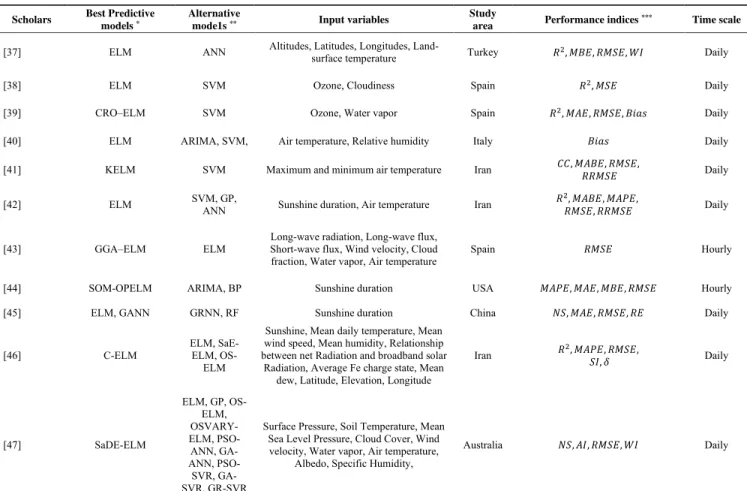
As review report, which is presented in Table 1, it is revealed that, there is an increasing trend in prediction of solar radiation using ELM while there are a very few researches which explore the efficiency of ELM in arid or semi-arid area. Therefore, herein, it was used to predict the G in a semi-arid area as Lower Cheliff plain in Algeria. The main goal of this study is to assess the capability of ELM model in prediction of daily G over the study site located at the Lower Cheliff region in Algeria. The obtained results of ELM were compared with two classic methods such as multiple linear regression (MLR) and autoregressive integrated moving aver-age (ARIMA) which are applied widely for solar radiation prediction. Furthermore, this study evaluates the minimum and maximum peak solar radiation where those are the main contributor elements for multiple energy applications.
TABLE 1. The studies reviewed in the application of the ELM models, relative to alternative models used in the prediction of solar radiation.
II. THEORY OF FORECASTING MODEL
A. EXTREME LEARNING MACHINE (ELM)
Based on the earlier data-driven models such as support vector machine (SVM) and artificial neural network (ANN), ELM model is a newer and a more efficient data-driven mechanism, as a modern single layer feed-forward network (SLFN) mechanism. Basically, an ELM model operates rela-tive to the feed-forward back propagation ANN (FFBP-ANN) and support vector machines. Moreover, an ELM model is more accurate and can solve problems in lesser time than an ANN or SVM [48], and thus has been applied in this study. In an ELM model, the biases (and weights) are selected randomly resulting in a distinct least-square solution. Using predictors and predictand matrix, an ELM solves the Moore-Penrose inverse function [33]. It uses a simplified three-step process that does not require a parameter search process like an SVM or ANN model. Instead, ELM requires the randomized identification of hidden neurons. Due to a higher prospect for real-time application, an ELM proffers a unique importance as compared to ANN models that possess ineffective convergence rates, local minima issues, inferior
generalization, iterative tuning process, and over-fitting of data. The improved and fast output of an ELM is important in real-time implementation [49], and could be very useful for spatiotemporal assessment of solar energy potential.
To develop an ELM model, we determine the architec-ture by an automatic process where a mathematical equa-tion (a piecewise continuous and differentiable) is applied to the data attributes using randomly assigned biases and weights (from a continuous probability distribution). Next, we elucidate a linear equation. While an ELM model has gained attention in atmospheric, climate and energy applications [43], [50]–[54], this manuscript is the first ever to apply this algorithm for forecasting solar radiation in Lower Cheliff plain, Algeria.
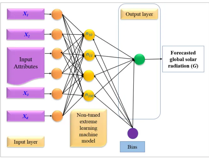
In Figure 1, the topology of an ELM is sketched. In this study, ELM was employed to train target/predictor pairs ((x1, y1), (x2,y2),. . ., (xi,yi)) withxirepresenting the predictors andyidenoting the predictand (G). The vector (x1,x2,. . .,xi) comprised of St, Tmax, Tmin, Tmean, RH, and U from which the patterns for future evolution of global solar radiation were extracted, while the predictand (y1, y2. . .yi) represents
FIGURE 1. A basic topology of an extreme learning machine model with d-dimensional input vectorX1,X2. . .Xd.
the response (G denotes target matrix). In a series of d-dimensional matrices, i=1, 2,. . ., N training parameters, xi<d andyi<. Huang et al. (2006a) mathematically indi-cated SLFN with L hidden neurons as:
fL(x)= L X
i=1
βihi(x)=h(x)β (1)
whereβ =[β1, β2. . . βL]T represents the output weight of matrix within the output and hidden neurons, h(x) =
[h1, h2. . . h L(x)] represents the outputs of hidden neuron which denotes the randomized hidden characteristics of the predictor xi, hi(x) represents ith hidden neuron. In addition, the response functions in hidden neurons may not be unique, and mostly, hi(x) can be represented as [48]:
hi(x)=G(ai,bi,x) ,aiRd,biR (2)
G (ai, bi, x) which indicates the hidden neuron variables (a,b) is a non-linear characteristic that needs to content ELM approximation theorem [55]. In an ELM model, an activation function was determined for the hidden layer to optimize the algorithm. In this study, the commonly used logarithmic sigmoid activation function from the MATLAB toolbox was
applied as described in equation below [56], [57]:
Log Sigmoid⇒G(a,b,x)= 1
1+exp(−ax+b) (3) In order to generalize the data used for the predicting G, a dual process is facilitated, where the random feature mapping is performed within the feature space, and a linear parameter solving is undertaken. As described by Huang et al. 2015, the error is minimized by resolving the weights joining the output (β) and hidden layer by employing least square fitting [48]:
minβ∈RI×MkHβ−Tk2 (4)
In Eq. (4),||represents Frobenius norm and H denotes matrix for randomized output of hidden layer [48]:
H= g(x1) ... g(xN) = g1(a1x1)+b1. . . ... g1(aNxN)+b1. . . gL(aLx1)+bL ... gL(aLxN)+bL (5)
The chosen matrix in the data training period is represent in the equation below [48]:
T = t1T ... tNT = t11... ... tN1. . . t1m tNm (6)
The optimal value is obtained by resolving the linear equations in the system, this is presented in the equation below [58]:
β∗=
H+T (7)
where H+ denotes the Moore-Penrose generalized inverse function (+) [59].
In this study, G forecasts denoted asyˆare obtained using test input vector (xtest) which is outside of training input data [33]: ˆ y= ∧ X i=1 ∧ βhi(aixtest+bi) (8)
B. MULTIPLE LINEAR REGRESSION (MLR)
To investigate the preciseness of an ELM model, the MLR model was developed. It is an adjunct of the simple regression model to multivariate input whereby a model is deduced to describe explicitly the changes in predictor data to evaluate their regression coefficients. In addition, this model makes certain that only little changes are withdrawn from the model because of unexplored ‘‘noise’’.
N represents the observations for d-dimensional predictor parameters. Equation below describe the regression expres-sion for MLR [60]:
Y =C+β1X1+β2X2+. . .+βdXd (9) where Y (N × 1) indicates objective variable matrix (G), X (N ×d) denotes a vector of the predictor variable(s), C represents y-intercept andβ denotes the multiple regression coefficient of individual regressor parameter(s) [61].
The magnitude of β for each predictor is estimated from least squares as described previously [62]. In the case of forecasting, the MLR fits the model to a series of Y andX matrix of the training duration. The fitted MLR through its y-intercept and coefficients is utilized in generating predicted values forY, in addition to set ofXvalues in testing (or cross-validation) duration. Previous studies had explained more about MLR [60], [63].
C. AUTO-REGRESSIVE MOVING INTEGRATED AVERAGE MODEL(ARIMA)
Another model used for evaluating ELM was the ARIMA model. ARIMA operates through univariate predictor time-series sectioned in an input/target subset. The model errors and time-lagged information are used for identifying complex structures in the original G data. Thus, an ARIMA model is important for multiple predictor data needed which other data-driven models including MLR or ELM does not possess. These variables (d, q, p) control ARIMA, whereby d repre-sents the number of non-seasonal differences; q is the number of lagged error and p indicates the number of autoregressive terms. There are three steps involved in the development of the ARIMA model, it includes forecasting, estimation and identification. An ARIMA (d, q, p) procedure is explained
in the equation below [64]:
9p(B)(1−B)dYt =δ+θqBεt (10)
whereYt is the original predictor, B denotes the backshift operator,εtrepresents the random perturbation (white noise) with a constant variance, covariance and zero mean),ψpis the autoregressive variable of orderp,δrepresents constant value,dindicates the differencing order employed in the non-seasonal or regular section of the series, andθqis the moving average variable of orderq.
In the implementation of an ARIMA model, the differenc-ing variable (d) is obtained through partial autocorrelation and autocorrelation to verify the ‘tailing off’ pattern and validate if a differencing is required for non-stationary data. qandpparameters are pinpointed for ‘trial’ models through maximum likelihood estimation (MLE) for examining the variables that most influence the probability for achieving data through least squares. The maximum log likelihood which referred to as the logarithm of observed data prob-ability generated from the estimated model is utilized for evaluating variable. Akaike’s Information Criterion (AIC) is employed for establishing ARIMA model by taking into consideration the immensity of MLE, correlation coefficients and the variance jointly examined in training data [8]:
AIC= −2log(L)+2(p+q+k+1) (11) where L denotes the log-likelihood of data, k=0 if c=0 and k=1 if c6=0 and last term in brackets represent the number of variables (including the variance of residual).
III. MATERIALS AND METHODS
A. STUDY AREAS AND METEOROLOGICAL DATA ACQUISITION
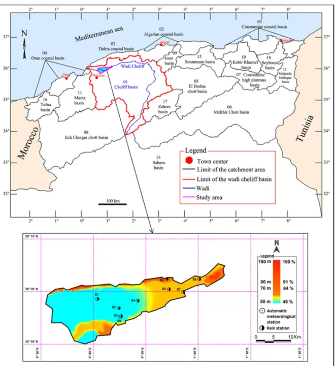
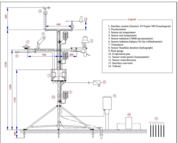
The Lower Cheliff Plain comprises of over 40,000 ha of land area, is situated in the Cheliff Basin in Northwest Algeria within the latitudes 34◦0301200and 36◦0505700N and longi-tudes 0◦40 and 01◦0600800E [65] (See Figure 2). The climate of Lower Chéliff is a semi-arid that possesses mean annual rainfall of 250 mm, low winter temperatures and very hot summers [65]. The result of the pedological investigations in this region [66], [67] showed that the region has the limey soil of clayey texture. The soils comprise a unique level of sodicity and temporary hydromorphy bind to the wet period. The dataset employed in this finding was obtained from Hmadna station in northern Algeria (Figure 3). The sta-tion is located Latitude: 35◦55’31’’ Nord and Longitude, 00◦45’04’’ Est within 50 m. The meteorological data used in this study consisted of daily observations of maximum, minimum and mean air temperatures (Tmax, Tmin, Tmean), daily mean relative humidity (RH), wind speed (Ws), sun-shine duration (Sd) and global radiation. The days with insuf-ficient data were eliminated from the structures in order to provide a consistence data span for the prediction process. The statistical climatic data variables are presented in Table 2, whereby the Xmean, Xmin, Xmax, Cv, and Sx represent
FIGURE 2. Study area location displayed the lower cheliff plain.
the mean, minimum, maximum, variation coefficient, and standard deviation, respectively.
B. PREDICTIVE MODEL DEVELOPMENT
All predictive models were generated using MATLAB envi-ronment under a Pentium 4, 2.93 GHz system. The main objective of this study was to examine the efficiency of extreme learning machine (ELM) model for forecasting global incident solar radiation. The focus was to evaluate the training data to develop the ELM model and then verify data to investigate its effectiveness. Since no set rule exists for
the data divisions, the partition of data preceding the usual procedure that researchers implement using divisions amidst train and test sets.
In this study, data sets obtained from a site located at the northern part of the Cheliff Basin in Northwest Algeria with daily meteorological data. The time series from 01-Jan-2006 to 31 Dec-2011 were sectioned into∼67 % (1-Jan-2006 to 31-Dec-2009) to the train and remainder∼33 % into the test set. Normally, for the predictive models, all input parameters were standardized. The input parameters were tested using cross-correlation analysis between the coefficient of solar
FIGURE 3. Automatic meteorological station of Hmadna used in this study.
radiation and sunshine hours St; evaporation ET; maximum, maximum, mean temperature (Tmax, Tmin, Tmean), and wind speed U.
In order to develop the EML model, mean, standard deviation, minimum, and maximum were computed for global solar radiation; G, sunshine hours St; evaporation ET; minimum, maximum, mean temperature (Tmax, Tmin, Tmean), and wind speed U. Seven models were developed by includ-ing each additional input variable in the models. The optimal model had all input variables resulting in a 7-12-1 (Input-Hidden-Output) neurons.
Fifteen models were developed for ARIMA, the best of which was ARIMA (3, 1, 2). MLR model also had seven mod-els with each including an additional regression parameter. The optimal model included all input variables in the form of regression parameters.
C. PERFORMANCE EVALUATION
Evaluation of model through American Society for Civil Engineers (Hydrology, 2000) advocates two categories of performance measures: descriptive and visual statistics. The forecasted and observed data were used to examine the maxi-mum, minimaxi-mum, mean, standard deviation, variance, kurto-sis, and skewness while the more standardized metrics are
employed to predict and verify the observed data in the test set. To establish whether an ELM model qualifies to predict the daily worldwide solar radiation in the study region, sta-tistical errors through mean absolute error (MAE), root mean square error (RMSE), correlation coefficient (r), relative (%) error data (RMSE and MAE), and Willmott’s Index (d) were applied as follows [69]:
1. The correlation coefficient (r) is given in the equation below: r=[ PN i=1 GOBS,i− ¯GOBS,i GFOR,i− ¯GFOR,i q PN i=1GOBS,i− ¯GOBS,i 2qPN i=1GFOR,i− ¯GFOR,i 2] (12) 2. Root mean square error (RMSE) is given in the equation
below: RMSE = v u u t 1 N N X i=1 GFOR,i−GOBS,i 2 (13) 3. Mean absolute error (MAE) is given in the equation below:
MAE= 1 N N X i=1 GFOR,i−GOBS,i (14)
TABLE 2. (a) Details of the experimental measurements, and the measuring range of the sensors (SYNMET Automatic Weather Station). (b) Daily statistics (01-01-2006 to 31-12-2012) for variables used to develop extreme learning machine model. c) Details of dataset used for model development.
4. Willmott’s Index (d) is given in the equation below: d= " PN i=1 GOBS,i−GFOR,i2 PN i=1 GFOR,i− ¯GOBS,i + GOBS,i− ¯GOBS,i 2 # (15) 5. Relative root mean square error (RRMSE¸%) is given in
the equation below:
RRMSE= q 1 N PN i=1 GFOR,i−GOBS,i 2 1 N PN i=1 GOBS,i (16)
6. Mean absolute percentage error (MAPE; %), is given in the equation below:
MAPE= 1 N N X i=1 GFOR,i−GOBS,i GOBS,i ×100 (17) 7. Nash Efficiency (E) is given in the equation below:
E =1− " PN i=1 GOBS,i−GFOR,i2 PN i=1 GOBS,i− ¯GOBS,i 2 # (18)
whereGFOR andGOBS are the forecasted and observed ith values of G,G¯FORandG¯OBSrepresent the mean G values of the forecasted and observed in the tested sample set and N denotes the number of datum points in the set.
IV. APPLICATION RESULTS AND DISCUSSION
A. INPUT VARIABILITY ANALYSIS
In this section, results attained from ELM, MLR and ARIMA for predicting global solar radiation are assessed to validate their adequacy in solar radiation modeling. The candidate study site selected for the investigation is located at the northern part of Cheliff Basin in Northwest Algeria with daily scale meteorological data for the period 01-Jan-2006 to 31-Dec-2011. The G predicted using ELM, MLR and ARIMA are analysed where the importance of input vari-ables is investigated in terms of the predictive accuracy. These models are compared, based on statistical perfor-mance criteria, including an analysis of model accuracy. In particular, the ELM model as a new non-tuned intelligent predictive model, is evaluated against the MLR and ARIMA for predicting G.
FIGURE 4. Boxplot of normalized target and input variables.
TABLE 3. Importance of inputs viz cross correlation of solar radiation with predictor (sunshine hrs St; evaporation ET; maximum, maximum, mean temperature (Tmax, Tmin, Tmean) and wind speed U).
To assess the quality of input variables, their variabilities are compared with together. As the input data have differ-ent ranges, thus data normalization is a useful technique to enhance the better perspective. Hence, the employed dataset was standardized between 0-1 as follows:
´
xi= (
xi−xmin) (xmax−xmin)
(19) where,x´iis theithnormalized value of predictive variable (x). To compare the variability of input variables, the inter quantile ranges (IQR) are computed using respected quartiles (Q75%-Q25%) as presented in Figure 4.
Figure 4 indicates the IQR of the normalized input vari-ables which are in rang of 0.15 to 0.51. Further, St(IQR
= 0.51) and U(IQR = 0.15) have the highest and lowest variability compare to other input variables.
B. MODELING PREDICTION ASSESSMENT
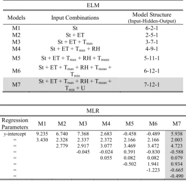
Prior to exhibit the statistical results of the predictive mod-els, it is worth to display the basic model architectures. Table 4 presents the optimal structure for the ELM, MLR and ARIMA models where ELM and MLR models indicate M7 is the optimum input combination. Whereas, ARIMA model acts differently in accordance to the internal param-eters (i.e.,p=autoregressive,d =differencing,q=moving average) and M14 was found to be the best model for ARIMA. Table 5 shows the optimal model (boldfaced)
performance metrics for the three predictive models and all constructed input combinations. The results indicate sunshine hours (correlation 0.903), evaporation (correlation 0.851) and maximum temperature (correlation 0.775) as most influential variables for the prediction process. The impact on perfor-mance metrics upon choosing the input variables into the three models of ELM, MLR and ARIMA was investigated in order to measure the performance of the models. Various input combinations were constructed to compare the per-formance of the three models. The ELM model has shown an excellent performance against MLR and ARIMA. With M7 input combination (by incorporating all the predictors), ELM’s best model results are correlation coefficient 0.978, Willmott’s Index 0.977, Nash Efficiency 0.956 with lowest Relative Root Mean Square Error of 9.58% and Relative Mean Absolute Error of 13.52%. On the same vein, MLR behaved similarly using the same input combination and had a comparable results of correlation coefficient 0.962, Willmott’s Index 0.961, Nash Efficiency 0.926 with a signifi-cantly higher Relative Root Mean Square Error of 12.38 % and Relative Mean Absolute Error of 17.48%. ARIMA’s best model (M14) model had much lower efficiency values, correlation coefficient 0.846, Willmott’s Index 0.834, Nash Efficiency 0.714 with the most significantly higher Relative Root Mean Square Error of 24.31 % and Relative Mean Absolute Error of 38.70 %.
The scenario of input combination between ELM and MLR were same, taking into consideration all variables for optimum results. Although MLR performance metrics were better than ARIMA, it was still significantly lower than ELM. The results showed ELM as the superior model when com-pared to MLR and ARIMA in predicting G. Quantitatively, ELM model displays results augmentation for instance RMSE and MAE reduced by 22.6 and 28.3% over the MLR model.
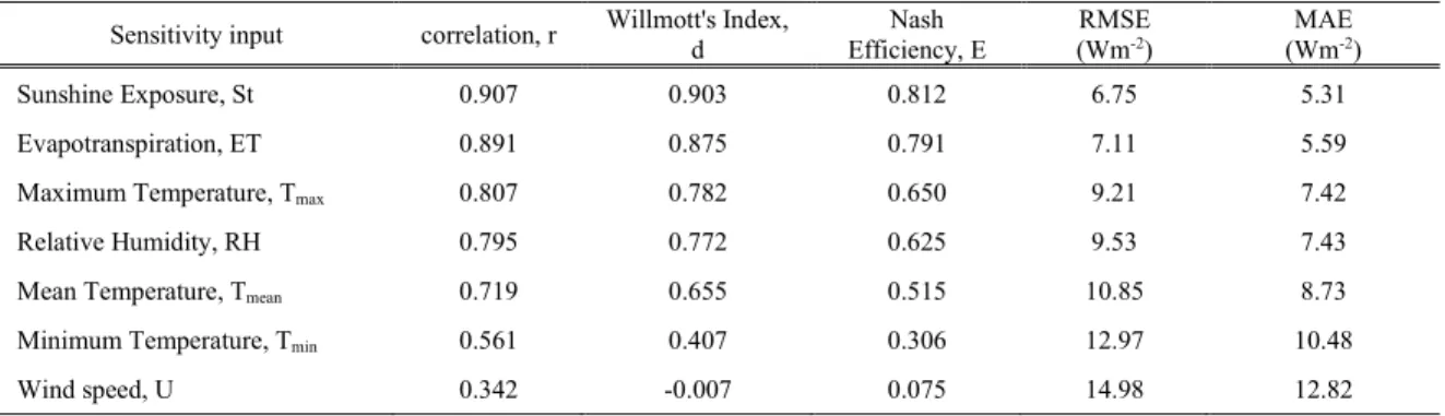
An interesting visualization for the performance of the ELM model should be done through studying the sensitivity analysis of each single predictor toward the G. The sensitivity analysis of ELM performance based on single predictor vari-ables were carried out and ranked by the accuracy of their performance (Table 6). Among the sensitivity inputs, Sun-shine Exposure (St) had the best correlation with value r≈
0.907, higher Willmott’s Index 0.903, higher Nash Efficiency 0.812 with Root Mean Square Error of 6.75 and Mean Abso-lute Error of 5.31. The wind speed showed the least impact variability on prediction with correlation 0.342, very poor Willmott’s Index -0.07 and Nash Efficiency of 0.075 with highest Root Mean Square Error 14.98 and Mean Absolute Error of 12.82. The poor impact is due to the characteristic of obtained data for wind speed which is at the depth of two meters. Hence it is not reliable enough in the phenomena of the incident solar radiation. Table 6 summarizes the ranking of all single predictors.
The three models of ELM, MLR and ARIMA were evalu-ated to determine the model error for predicting peak (max-imum and min(max-imum G) values. It can be noted that the
TABLE 4. ELM, MLR and ARIMA model architecture and parameters with optimal model in boldface.
prediction of the peak values is the most significant concern the energy cell engineering designers. Hence, focusing on this is highly reliable aspect in the analysis. Here again, the results show the significant predictability of ELM perfor-mance in predicting the maximum and minimum values in most instances with lower error values when compared over the MLR and ARIMA models. Table 7 shows the model errors
where the least error in ELM instance is shown in bold red. The statistical values of the predicted G were computed. The values show the absolute difference of the three models with respect to the observed G in the testing period (Table 8).
A graphical evaluation of the developed models’ perfor-mance can be made by plotting the predicted values against the real measured data in the form of scatterplot. As such,
TABLE 5. Evaluation of extreme learning machine (ELM) with multiple linear regression (MLR) and autoregressive integrated moving average (ARIMA) model. Note: Optimal model is boldfaced.
TABLE 6. Sensitivity analysis of extreme learning machine performance based on single predictors variables ranked by the accuracy of performance.
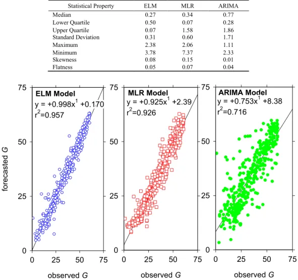
Figure 5 presents the variance diversion from the ideal line 45o (predicted verses measured G values) using ELM, MLR and ARIMA models based on the optimal predictor metrolog-ical information M7 for ELM and MLR and M14 for ARIMA models. The MLR performs better than the ARIMA model with a better correlation. However, it is quite clearly evident
that ELM is the better model with a much higher correlation between predicted and observed values.
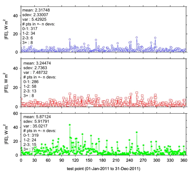
Figure 6 shows the time series of the test point’s data from (1stJan 2011 to 31stDecember 2011). The ELM case shows in the first graph (blue) much better statistical values, standard deviation 2.3307 and variance of 5.42925 when
TABLE 7. Evaluation of model error (Wm−2) for forecasting peak (maximum and minimum G values).
TABLE 8. Statistical properties of predicted global solar radiation (G) (Wm−2) presented as the absolute difference of ELM, MLR and ARIMA models with respect to the observed G in test period.
FIGURE 5. Scatterplots of the observed and predicted global solar radiation (G) over the testing period.
compared with MLR, standard deviation 2.7363 and vari-ance of 7.48732. Whereas, ARIMA model has significantly a higher standard deviation 5.91791 and variance of 35.0217.
Overall, when all performance metrics and general statistical properties shown are considered, ELM exhibit significantly better forecasting ability for global solar radiation.
FIGURE 6. Forecasting error,|FE|in test period for ELM compared with MLR and ARIMA model. In each panel, the error statistic (mean, standard dev, variance and number of points (n) in±n sdev are also shown).
The importance of accurate and precise solar radiation data in many solar energy applications is crucial. These data are imperative in the design of photovoltaic panels, solar drying systems, solar air heaters, furnaces, and many other energy implementations. This study confirms the feasibility and predictability of the ELM as an efficient model for pre-dicting solar radiation modeling. This study can be extended to include for instance natural inspired optimizer for the input variables where the investigation for the correlated attributers toward the G is highly significant to be recognized and par-ticularly for the studied region.
C. MODELING VALIDATION AGAINST THE LITERATURE
To have fair assessment of the proposed predictive ELM model in predicting the global solar radiation, the obtained results are compared with previous conducted researches over Africa region and others. In this manner, a reasonable assess-ment is performed to validate the accuracy of proposed model in predicting the global solar radiation [70]–[75]. Guermoui
and Rabehi [72] evaluated two AI models called Gaussian process regression methodology (GPR) and least square sup-port vector machine (LS-SVM) to predict the global solar radiation over Ghardaia region of Algeria.
To achieve the optimistic model, GPR and two differ-ent LS-SVM models with differdiffer-ent Kernel functions were investigated using same predictive variables. The obtained results of those models showed values of determination of coefficient (R2) in range of [0.87∼0.91]. Sharafatiet al.[70] proposed couple machine learning models such as Ran-dom Forest (RF), RanRan-dom Tree (RT), Reduced Error Prun-ing Trees (REPT), and Random committee integrated with Random Tree reduce (RC) to simulate solar radiation over Burkina Faso. Authors examined combinations of seven pre-dictive variables to achieve the realistic models. Based on the obtained values of error indices, it can be concluded that the R2index of developed models were within the range of [0.66-0.93] and the highest performance attained using RF model (R2=0.93). Taoet al.[71] examined the potential of
a newly hybrid ELM model called self-adaptive evolutionary extreme learning machine (SaE-ELM) to predict daily solar radiation using eight different combinations of input vari-ables over the Burkina Faso region. The results indicated the developed SaE-ELM models have higher accuracy in term of R2within range of 0.49 to 0.947 over different employed stations. In another study, a hybrid between Firefly algorithm and SVM model for stations (Iseyin, Maiduguri: Nageria) has attained results lower than our proposed model in terms of R2=0.795 and R2=0.518 respectively [76]. Fanet al.[73] presented a comparison study between SVM and XGBoost for predicting global solar radiation based air temperature and rainfall within humid ‘‘subtropical climate’’ in China. The researchers found that the best prediction results attained for the testing phase using the SVM model with R2 =0.76 while the best results attained using the XGBoost model achieved R2=0.74. Dahmaniet al.[74] utilized a multi-layer perceptron model for estimating 5-min and hourly horizontal global irradiation from exogenous meteorological data within Algeria. The study conducted based on wide range of input combinations (i.e., 1023). The investigation reported good predictability performance with R2 =0.96 for the incorpo-ration 10 input variables. Although the proposed model was able to attain almost similar to the current research capacity, the developed was integrated with feature selection approach as a filter for the correlated predictors. In addition, the inves-tigated horizon scale (i.e., hourly and 5-min) is different from the present. In other study, the potential of the boosted regression trees (BRT) model for predicting solar irradiance based on fusing spatial and temporal information [75]. The results evidence the capability of the introduced BRT model with magnitude of R2=0.91. Having assessed the conducted researches over the literature, it is evidence that the proposed predictive model and input variables have better performance (R2 =0.956) in predicting global solar radiation compared to literature studies over Africa region and others.
V. CONCLUSION
Over the past couple decades, estimation and predicting future values of solar radiation in various sites was a chal-lenge mission for researchers and scientists. This is due to the fact that solar radiation is highly stochastic climatolog-ical element that is influenced by various other associated parameters. Hence, exploring a reliable predictive modeling strategy is still the passionate of the scholars up to date. This paper has proposed a set of extreme learning predictive model for daily solar radiation scale coordinated in the northern part of Cheliff Basin at the Northwest part of Algeria. Daily mete-orological data over the period 01-Jan-2006 to 31-Dec-2011 were assessed to validate their adequacy in solar radiation modeling. The successful results reported in the paper were accomplished in several steps. The impact on performance metrics upon choosing the input variables into the proposed and the comparable models was investigated in order to gauge the performance of the models. Various input combinations based on multiple meteorological information were used to
compare the performance of the three models. The ELM model has shown an excellent performance against MLR and ARIMA models. Incorporating all the input parameters (7th input combination), the ELM’s best model results are correlation coefficient 0.978, Willmott’s Index 0.977, Nash Efficiency 0.956 with lowest Relative Root Mean Square Error of 9.58% and Relative Mean Absolute Error of 13.52%. In addition, the three models of ELM, MLR and ARIMA were evaluated to determine the model error for predicting the peak magnitudes (maximum and minimum of G). The results also showed that ELM had better predictability for the maximum and minimum values in most instances with lower error values. In conclusion, the modeling strategy approach exhibited a reliable one that can be applied as real time global radiation quantification for Algeria region. The current research can be further extended through including some nature inspired optimization algorithm for input variables selection as prior step for the prediction procedure [77]–[79]. CONFLICTS OF INTEREST
The authors declare no conflict of interest. ACKNOWLEDGMENT
The authors very much thankful for the respected reviewers for their constructive comments. Our appreciation is extended to the editor-in-chief and associate editor for handling our manuscript.
REFERENCES
[1] U. Economic and S. Council, ‘‘Progress towards the sustainable develop-ment goals,’’ New York, NY, USA, Tech. Rep., 2017.
[2] T. Khatib, A. Mohamed, and K. Sopian, ‘‘A review of solar energy modeling techniques,’’ Renew. Sustain. Energy Rev., vol. 16, no. 5, pp. 2864–2869, Jun. 2012.
[3] L. M. Halabi, S. Mekhilef, and M. Hossain, ‘‘Performance evaluation of hybrid adaptive neuro-fuzzy inference system models for predicting monthly global solar radiation,’’Appl. Energy, vol. 213, pp. 247–261, Mar. 2018.
[4] A. K. Yadav and S. Chandel, ‘‘Tilt angle optimization to maximize inci-dent solar radiation: A review,’’Renew. Sustain. Energy Rev., vol. 23, pp. 503–513, Jul. 2013.
[5] A. F. Zobaa and R. C. Bansal,Handbook of Renewable Energy Technology. Singapore: World Scientific, 2011.
[6] A. Voskrebenzev, S. Riechelmann, A. Bais, H. Slaper, and G. Seckmeyer, ‘‘Estimating probability distributions of solar irradiance,’’Theor. Appl. Climatol., vol. 119, nos. 3–4, pp. 465–479, Feb. 2015.
[7] K. Mohammadi, S. Shamshirband, D. Petkovi, and H. Khorasanizadeh, ‘‘Determining the most important variables for diffuse solar radiation prediction using adaptive neuro-fuzzy methodology; case study: City of Kerman, Iran,’’ Renew. Sustain. Energy Rev., vol. 53, pp. 1570–1579, Jan. 2016.
[8] S. Pappas, L. Ekonomou, D. Karamousantas, G. Chatzarakis, S. Katsikas, and P. Liatsis, ‘‘Electricity demand loads modeling using AutoRegressive Moving Average (ARMA) models,’’Energy, vol. 33, no. 9, pp. 1353–1360, Sep. 2008.
[9] S. Mohanty, P. K. Patra, and S. S. Sahoo, ‘‘Prediction and applica-tion of solar radiaapplica-tion with soft computing over tradiapplica-tional and conven-tional approach—A comprehensive review,’’Renew. Sustain. Energy Rev., vol. 56, pp. 778–796, Apr. 2016.
[10] B. Mccune and D. Keon, ‘‘Equations for potential annual direct incident radiation and heat load,’’J. Vegetation Sci., vol. 13, no. 4, pp. 603–606, Aug. 2002.
[11] N. T. Nikolov and K. F. Zeller, ‘‘A solar radiation algorithm for ecosystem dynamic models,’’Ecological Model., vol. 61, nos. 3–4, pp. 149–168, Jun. 1992.
[12] J. Almorox and C. Hontoria, ‘‘Global solar radiation estimation using sunshine duration in Spain,’’ Energy Convers. Manage., vol. 45, nos. 9–10, pp. 1529–1535, Jun. 2004.
[13] A. Angstrom, ‘‘Solar and terrestrial radiation. Report to the international commission for solar research on actinometric investigations of solar and atmospheric radiation,’’Quart. J. Roy. Meteorol. Soc., vol. 50, no. 210, pp. 121–126, Jul. 2010.
[14] R. Benson, M. Paris, J. Sherry, and C. Justus, ‘‘Estimation of daily and monthly direct, diffuse and global solar radiation from sunshine duration measurements,’’Solar Energy, vol. 32, no. 4, pp. 523–535, 1984. [15] J. A. Prescott, ‘‘Evaporation from a water surface in relation to solar
radiation,’’Trans. Roy. Soc. S. Aust., vol. 46, pp. 114–118, 1940. [16] E. O. Falayi, J. O. Adepitan, and A. B. Rabiu, ‘‘Empirical models for the
correlation of global solar radiation with meteorological data for Iseyin, Nigeria,’’Int. J. Phys. Sci., vol. 3, no. 9, pp. 210–216, 2008.
[17] D. W. Medugu and D. Yakubu, ‘‘Estimation of mean monthly global solar radiation in Yola-Nigeria using angstrom model,’’Adv. Appl. Sci. Res., vol. 2, no. 2, pp. 414–421, 2011.
[18] Y. Jiang, ‘‘Estimation of monthly mean daily diffuse radiation in China,’’ Appl. Energy, vol. 86, no. 9, pp. 1458–1464, Sep. 2009.
[19] H. Khorasanizadeh, K. Mohammadi, and M. Jalilvand, ‘‘A statistical com-parative study to demonstrate the merit of day of the year-based models for estimation of horizontal global solar radiation,’’Energy Convers. Manage., vol. 87, pp. 37–47, Nov. 2014.
[20] K. K. Kuok, S. M. Kueh, and P. C. Chiu, ‘‘Bat optimisation neural networks for rainfall forecasting: Case study for Kuching city,’’J. Water Climate Change, vol. 10, no. 3, pp. 569–579, Sep. 2019.
[21] Y. Liu, Y.-F. Sang, X. Li, J. Hu, and K. Liang, ‘‘Long-term streamflow forecasting based on relevance vector machine model,’’Water, vol. 9, no. 1, p. 9, Dec. 2016.
[22] T.-Y. Pan, Y.-T. Yang, H.-C. Kuo, Y.-C. Tan, J.-S. Lai, T.-J. Chang, C.-S. Lee, and K. H. Hsu, ‘‘Improvement of watershed flood forecasting by typhoon rainfall climate model with an ANN-based southwest monsoon rainfall enhancement,’’J. Hydrol., vol. 506, pp. 90–100, Dec. 2013. [23] Z. M. Yaseen, M. Fu, C. Wang, W. H. M. W. Mohtar, R. C. Deo, and
A. El-shafie, ‘‘Application of the hybrid artificial neural network coupled with rolling mechanism and grey model algorithms for streamflow fore-casting over multiple time horizons,’’Water Resour. Manage., vol. 32, no. 5, pp. 1883–1899, Mar. 2018.
[24] M. A. Ghorbani, R. C. Deo, Z. M. Yaseen, M. H. Kashani, and B. Mohammadi, ‘‘Pan evaporation prediction using a hybrid multilayer perceptron-firefly algorithm (MLP-FFA) model: Case study in North Iran,’’ Theor. Appl. Climatol., vol. 133, nos. 3–4, pp. 1119–1131, Aug. 2018.
[25] Z. Abdulelah Al-Sudani, S. Q. Salih, A. Sharafati, and Z. M. Yaseen, ‘‘Development of multivariate adaptive regression spline integrated with differential evolution model for streamflow simulation,’’ J. Hydrol., vol. 573, pp. 1–12, Jun. 2019.
[26] H. Sanikhani, R. C. Deo, P. Samui, O. Kisi, C. Mert, R. Mirabbasi, S. Gavili, and Z. M. Yaseen, ‘‘Survey of different data-intelligent modeling strategies for forecasting air temperature using geographic information as model predictors,’’Comput. Electron. Agricult., vol. 152, pp. 242–260, Sep. 2018.
[27] M. Ali, R. C. Deo, N. J. Downs, and T. Maraseni, ‘‘Multi-stage hybridized Online sequential extreme learning machine integrated with Markov Chain Monte Carlo copula-bat algorithm for rainfall forecasting,’’Atmos. Res., vol. 213, pp. 450–464, Nov. 2018.
[28] S. Naganna, P. Deka, M. Ghorbani, S. Biazar, N. Al-Ansari, and Z. Yaseen, ‘‘Dew point temperature estimation: Application of artificial intelligence model integrated with nature-inspired optimization algorithms,’’Water, vol. 11, no. 4, p. 742, Apr. 2019.
[29] H. Liu, H.-Q. Tian, and Y.-F. Li, ‘‘Four wind speed multi-step forecasting models using extreme learning machines and signal decomposing algo-rithms,’’Energy Convers. Manage., vol. 100, pp. 16–22, Aug. 2015. [30] V. Nikoli, S. Motamedi, S. Shamshirband, D. Petkovi, S. Ch, and
M. Arif, ‘‘Extreme learning machine approach for sensorless wind speed estimation,’’Mechatronics, vol. 34, pp. 78–83, Mar. 2016.
[31] S. S. Abdullah, M. Malek, N. S. Abdullah, O. Kisi, and K. S. Yap, ‘‘Extreme learning machines: A new approach for prediction of reference evapotranspiration,’’J. Hydrol., vol. 527, pp. 184–195, Aug. 2015. [32] O. Kisi and M. Alizamir, ‘‘Modelling reference evapotranspiration using
a new wavelet conjunction heuristic method: Wavelet extreme learning machine vs wavelet neural networks,’’Agricult. Forest Meteorol., vol. 263, pp. 41–48, Dec. 2018.
[33] G.-B. Huang, Q.-Y. Zhu, and C.-K. Siew, ‘‘Extreme learning machine: The-ory and applications,’’Neurocomputing, vol. 70, nos. 1–3, pp. 489–501, Dec. 2006.
[34] L. Zhang, S. Wang, G.-B. Huang, W. Zuo, J. Yang, and D. Zhang, ‘‘Manifold criterion guided transfer learning via intermediate domain generation,’’IEEE Trans. Neural Netw. Learn. Syst., vol. 30, no. 12, pp. 3759–3773, Dec. 2019.
[35] L. Zhang and D. Zhang, ‘‘Robust visual knowledge transfer via extreme learning machine-based domain adaptation,’’IEEE Trans. Image Process., vol. 25, no. 10, pp. 4959–4973, Oct. 2016.
[36] L. Zhang and D. Zhang, ‘‘Evolutionary cost-sensitive extreme learn-ing machine,’’IEEE Trans. Neural Netw. Learn. Syst., vol. 28, no. 12, pp. 3045–3060, Dec. 2017.
[37] M. Şahin, ‘‘Comparison of modelling ANN and ELM to estimate solar radiation over Turkey using NOAA satellite data,’’Int. J. Remote Sens., vol. 34, no. 21, pp. 7508–7533, Nov. 2013.
[38] S. Salcedo-Sanz, C. Casanova-Mateo, A. Pastor-Sánchez, D. Gallo-Marazuela, A. Labajo-Salazar, and A. Portilla-Figueras, ‘‘Direct solar radiation prediction based on soft-computing algorithms including novel predictive atmospheric variables,’’ inProc. Int. Conf. Intell. Data Eng. Automated Learn.Berlin, Germany: Springer, Oct. 2013, pp. 318–325. [39] S. Salcedo-Sanz, C. Casanova-Mateo, A. Pastor-Sánchez, and
M. Sánchez-Girón, ‘‘Daily global solar radiation prediction based on a hybrid coral reefs optimization—Extreme learning machine approach,’’ Solar Energy, vol. 105, pp. 91–98, Jul. 2014.
[40] M. Lazzaroni, S. Ferrari, V. Piuri, A. Salman, L. Cristaldi, and M. Faifer, ‘‘Models for solar radiation prediction based on different measurement sites,’’Measurement, vol. 63, pp. 346–363, Mar. 2015.
[41] S. Shamshirband, K. Mohammadi, H.-L. Chen, G. Narayana Samy, D. Petkovi, and C. Ma, ‘‘Daily global solar radiation prediction from air temperatures using kernel extreme learning machine: A case study for Iran,’’J. Atmos. Solar-Terr. Phys., vol. 134, pp. 109–117, Nov. 2015. [42] S. Shamshirband, K. Mohammadi, P. L. Yee, D. Petkovi, and
A. Mostafaeipour, ‘‘A comparative evaluation for identifying the suitability of extreme learning machine to predict horizontal global solar radiation,’’Renew. Sustain. Energy Rev., vol. 52, pp. 1031–1042, Dec. 2015.
[43] A. Aybar-Ruiz, S. Jiménez-Fernández, L. Cornejo-Bueno, C. Casanova-Mateo, J. Sanz-Justo, P. Salvador-González, and S. Salcedo-Sanz, ‘‘A novel grouping genetic algorithm–extreme learning machine approach for global solar radiation prediction from numerical weather models inputs,’’Solar Energy, vol. 132, pp. 129–142, Jul. 2016. [44] Y. Wu and J. Wang, ‘‘A novel hybrid model based on artificial
neu-ral networks for solar radiation prediction,’’ Renew. Energy, vol. 89, pp. 268–284, Apr. 2016.
[45] Y. Feng, N. Cui, Q. Zhang, L. Zhao, and D. Gong, ‘‘Comparison of artificial intelligence and empirical models for estimation of daily diffuse solar radiation in North China Plain,’’Int. J. Hydrogen Energy, vol. 42, no. 21, pp. 14418–14428, May 2017.
[46] S. H. Hosseini Nazhad, M. M. Lotfinejad, M. Danesh, R. U. Amin, and S. Shamshirband, ‘‘A comparison of the performance of some extreme learning machine empirical models for predicting daily horizontal diffuse solar radiation in a region of southern Iran,’’Int. J. Remote Sens., vol. 38, no. 23, pp. 6894–6909, Dec. 2017.
[47] S. Ghimire, R. C. Deo, N. J. Downs, and N. Raj, ‘‘Self-adaptive differen-tial evolutionary extreme learning machines for long-term solar radiation prediction with remotely-sensed MODIS satellite and Reanalysis atmo-spheric products in solar-rich cities,’’Remote Sens. Environ., vol. 212, pp. 176–198, Jun. 2018.
[48] G. Huang, G.-B. Huang, S. Song, and K. You, ‘‘Trends in extreme learning machines: A review,’’Neural Netw., vol. 61, pp. 32–48, Jan. 2015. [49] N. Acharya, N. A. Shrivastava, B. K. Panigrahi, and U. C. Mohanty,
‘‘Development of an artificial neural network based multi-model ensemble to estimate the northeast monsoon rainfall over south peninsular India: An application of extreme learning machine,’’Climate Dyn., vol. 43, nos. 5–6, pp. 1303–1310, Sep. 2014.
[50] Ö. F. Ertuˇgrul and Y. Kaya, ‘‘A detailed analysis on extreme learning machine and novel approaches based on ELM,’’Am. J. Comput. Sci. Eng., vol. 1, no. 5, pp. 43–50, 2014.
[51] Y. Feng, N. Cui, L. Zhao, X. Hu, and D. Gong, ‘‘Comparison of ELM, GANN, WNN and empirical models for estimating reference evapotran-spiration in humid region of Southwest China,’’J. Hydrol., vol. 536, pp. 376–383, May 2016.
[52] I. Ebtehaj, H. Bonakdari, and S. Shamshirband, ‘‘Extreme learning machine assessment for estimating sediment transport in open channels,’’ Eng. Comput., vol. 32, no. 4, pp. 691–704, Oct. 2016.
[53] Y. Bai, M. Wong, W.-Z. Shi, L.-X. Wu, and K. Qin, ‘‘Advancing of land surface temperature retrieval using extreme learning machine and Spatio-temporal adaptive data fusion algorithm,’’Remote Sens., vol. 7, no. 4, pp. 4424–4441, Apr. 2015.
[54] B. Wang, S. Huang, J. Qiu, Y. Liu, and G. Wang, ‘‘Parallel Online sequen-tial extreme learning machine based on MapReduce,’’Neurocomputing, vol. 149, pp. 224–232, Feb. 2015.
[55] N.-Y. Liang, G.-B. Huang, P. Saratchandran, and N. Sundararajan, ‘‘A fast and accurate Online sequential learning algorithm for feedforward networks,’’IEEE Trans. Neural Netw., vol. 17, no. 6, pp. 1411–1423, Nov. 2006.
[56] Z. M. Yaseen, O. Jaafar, R. C. Deo, O. Kisi, J. Adamowski, J. Quilty, and A. El-Shafie, ‘‘Stream-flow forecasting using extreme learning machines: A case study in a semi-arid region in Iraq,’’ J. Hydrol., vol. 542, pp. 603–614, Nov. 2016.
[57] Z. M. Yaseen, R. C. Deo, A. Hilal, A. M. Abd, L. C. Bueno, S. Salcedo-Sanz , and M. L. Nehdi, ‘‘Predicting compressive strength of lightweight foamed concrete using extreme learning machine model,’’Adv. Eng. Softw., vol. 115, pp. 112–125, Jan. 2018.
[58] M. Hou, T. Zhang, F. Weng, M. Ali, N. Al-Ansari, and Z. Yaseen, ‘‘Global solar radiation prediction using hybrid Online sequential extreme learning machine model,’’Energies, vol. 11, no. 12, p. 3415, Dec. 2018. [59] H. Sanikhani, R. C. Deo, Z. M. Yaseen, O. Eray, and O. Kisi, ‘‘Non-tuned
data intelligent model for soil temperature estimation: A new approach,’’ Geoderma, vol. 330, pp. 52–64, Nov. 2018.
[60] N. R. Draper and H. Smith, Applied Regression Analysis, vol. 326. Hoboken, NJ, USA: Wiley, 1998.
[61] G. Civelekoglu, N. Yigit, E. Diamadopoulos, and M. Kitis, ‘‘Prediction of bromate formation using multi-linear regression and artificial neural networks,’’Ozone, Sci. Eng., vol. 29, no. 5, pp. 353–362, Oct. 2007. [62] M. Şahin, Y. Kaya, and M. Uyar, ‘‘Comparison of ANN and MLR models
for estimating solar radiation in Turkey using NOAA/AVHRR data,’’Adv. Space Res., vol. 51, no. 5, pp. 891–904, Mar. 2013.
[63] D. C. Montgomery, E. A. Peck, and G. G. Vining,Introduction to Linear Regression Analysis, vol. 821. Hoboken, NJ, USA: Wiley, 2012. [64] G. E. P. Box and G. M. Jenkins,Time Series Analysis, Forecasting and
Control, 1st ed. San Francisco, CA, USA: Holden-Day, 1970.
[65] A. E. K. Douaoui, H. Nicolas, and C. Walter, ‘‘Detecting salinity hazards within a semiarid context by means of combining soil and remote-sensing data,’’Geoderma, vol. 134, nos. 1–2, pp. 217–230, Sep. 2006.
[66] D. Saidi, a Douaoui, Y. Le Bissonnais, and C. Walter, ‘‘Sensibilité de la surface des sols des plaines du Chélif à la dégradation structurale,’’Etude Gest. des Sols, vol. 6, no. 1, pp. 15–25, 1999.
[67] C. Walter, A. B. Mcbratney, A. Douaoui, and B. Minasny, ‘‘Spatial predic-tion of topsoil salinity in the Chelif Valley, Algeria, using local ordinary kriging with local variograms versus whole-area variogram,’’Soil Res., vol. 39, no. 2, p. 259, 2001.
[68] ASCE Task Committee on Application of Artificial Neural Networks in Hydrology, ‘‘Artificial neural networks in hydrology. I: Preliminary concepts,’’J. Hydrol. Eng., vol. 5, no. 2, pp. 115–123, 2000.
[69] A. Sharafati, R. Yasa, and H. M. Azamathulla, ‘‘Assessment of stochastic approaches in prediction of wave-induced pipeline scour depth,’’ J. Pipeline Syst. Eng. Pract., vol. 9, no. 4, Nov. 2018, Art. no. 04018024.
[70] A. Sharafati, K. Khosravi, P. Khosravinia, K. Ahmed, S. A. Salman, Z. M. Yaseen, and S. Shahid, ‘‘The potential of novel data mining models for global solar radiation prediction,’’Int. J. Environ. Sci. Technol., vol. 16, no. 11, pp. 7147–7164, Nov. 2019.
[71] H. Tao, I. Ebtehaj, H. Bonakdari, S. Heddam, C. Voyant, N. Al-Ansari, R. Deo, and Z. M. Yaseen, ‘‘Designing a new data intelligence model for global solar radiation prediction: Application of multivariate modeling scheme,’’Energies, vol. 12, no. 7, p. 1365, Apr. 2019.
[72] M. Guermoui and A. Rabehi, ‘‘Soft computing for solar radiation poten-tial assessment in Algeria,’’Int. J. Ambient Energy, vol. 1, pp. 1–10, Aug. 2018.
[73] J. Fan, X. Wang, L. Wu, H. Zhou, F. Zhang, X. Yu, X. Lu, and Y. Xiang, ‘‘Comparison of support vector machine and extreme gradient boosting for predicting daily global solar radiation using temperature and precipitation in humid subtropical climates: A case study in China,’’Energy Convers. Manage., vol. 164, pp. 102–111, May 2018.
[74] K. Dahmani, G. Notton, C. Voyant, R. Dizene, M. L. Nivet, C. Paoli, and W. Tamas, ‘‘Multilayer Perceptron approach for estimating 5-min and hourly horizontal global irradiation from exogenous meteorological data in locations without solar measurements,’’Renew. Energy, vol. 90, pp. 267–282, May 2016.
[75] C. Huang, L. Wang, and L. L. Lai, ‘‘Data-driven short-term solar irradiance forecasting based on information of neighboring sites,’’IEEE Trans. Ind. Electron., vol. 66, no. 12, pp. 9918–9927, Dec. 2019.
[76] L. Olatomiwa, S. Mekhilef, S. Shamshirband, K. Mohammadi, D. Petkovi, and C. Sudheer, ‘‘A support vector machine–firefly algorithm-based model for global solar radiation prediction,’’Solar Energy, vol. 115, pp. 632–644, May 2015.
[77] S. Q. Salih and A. A. Alsewari, ‘‘A new algorithm for normal and large-scale optimization problems: Nomadic People Optimizer,’’Neural Com-put. Appl., pp. 1–28, 2019.
[78] H. A. Abdulwahab, A. Noraziah, A. A. Alsewari, and S. Q. Salih, ‘‘An enhanced version of black hole algorithm via Levy flight for optimization and data clustering problems,’’IEEE Access, vol. 7, pp. 142085–142096, 2019.
[79] S. Q. Salih, ‘‘A new training method based on black hole algorithm for convolutional neural network,’’J. Southwest Jiaotong Univ., vol. 54, no. 3, pp. 1–10, 2019.
TAO HAI received the B.Sc. degree from the Department of Computer and Information Sci-ence, Northwest University of Nationalities, in 2004, the M.S. degree from the School of Mathematics and Statistics, Lanzhou University, in 2009, and the Ph.D. degree from the Faculty of Computer System and Software Engineering, Uni-versity Malaysia Pahang, in 2012. He is currently an Associate Professor with the Baoji University of Arts and Sciences. His current research interests include machine learning, the Internet of Things, and optimization compu-tation.
AHMAD SHARAFATI received the master’s degree in water resources engineering studies from the Sharif University of Technology, in 2005, and the Ph.D. degree in water resources engineering studies from the Iran University of Science and Technology, in 2013. He is currently an Assistant Professor with the Department of Civil Engineer-ing, Science and Research Branch, Islamic Azad University. He has a diverse expertise on catch-ment engineering design and sustainability. He has several skills on the implementation of computer aid and advanced machine learning models.
ACHITE MOHAMMED received the Ph.D. degree in hydrology engineering, water resources engineering, hydrological processes modeling, environmental engineering and climate from the University of Science and Technology of Oran (USTO), Algeria, in 2007. In addition, he has an excellent expertise in artificial neural networks, advanced data analytics, and environmental sci-ences. He is currently a Senior Lecturer and a Senior Researcher in agronomy, environment and hydrology. He has published and presented in international conferences more than 75 articles, with a Google Scholar H-Index of 8, and a total of 347 citations.
SINAN Q. SALIH received the B.Sc. degree in information systems from the University of Anbar, Anbar, Iraq, in 2010, the M.Sc. degree in com-puter sciences from Universiti Tenaga National (UNITEN), Malaysia, in 2012, and the Ph.D. degree in soft modeling and intelligent systems from Universiti Malaysia Pahang (UMP). His cur-rent research interests include optimization algo-rithms, nature-inspired metaheuristics, machine learning, and feature selection problem for real world problems.
RAVINESH C. DEO is currently a Research Leader in predictive modeling with the Univer-sity of Southern Queensland, with proven exper-tise in artificial intelligence, decision-systems with machine learning heuristic and metaheuristic algorithms. He has undertaken knowledge exchange programs in Singapore, Japan, Europe, China, USA, Panama, and Canada, securing inter-national standing to research innovative problems in data-driven models and applications in energy, hydrology, climate, environment, and health sectors. He has more than 160 publications including 120 journals (mostly Scopus Quartile 1) with citations exceeding 2600 times, Google Scholar H-Index as 27, i-10 Index of 56 and Scopus H-Index of 25. He has published Edited Books with Elsevier, Springer Nature and IGI Global. He has supervised more than 10 Ph.D. and master’s Dissertation, and leads a team, to supervise more than 15 projects for the Doctor of Philosophy, Doctor of Applied Science, Master of Science Research, Master of Science dissertations and is the industry internship mentor for doctoral students. He was awarded internationally competitive Queensland Government (U.S.) Smithsonian Fellowship, Australia–China Young Scientist Exchange Award, Japan Society for Pro-motion of Science International Fellowship, Chinese Academy of Science Presidential Fellowship, and Australian Endeavour Fellowship. He received Publication Excellence Awards, Head of the Department Research and Executive Dean’s Teaching Awards, and Gold Medal for Academic Excel-lence (Bachelors), including School Dux of Fiji. He held Visiting Professor Roles at international institutions such as the Chinese Academy of Science, Northwest Normal University, Peking University, The University of Tokyo, Kyoto University, Kyushu University, The University of Alcala, and the National University of Singapore. He held Senior Scientist roles at McGill University and US Smithsonian Tropical Institute. Dr. Deo professionally affiliated at scientific bodies: Institute of Physics, Australian Mathematical Society, and Australasian Association for Engineering Education, Australia Global Alumni, and American Geophysical Union. Through international links, he mentors researchers at the Chinese Academy of Science. He is currently on Editorial Boards ofRemote Sensing & EnergiesSpecial Issue journals and officially serves as American Society for Civil Engineer’s Journal of Hydrologic Engineering.
NADHIR AL-ANSARI received the B.Sc. and M.Sc. degrees from the University of Baghdad, in 1968 and 1972, respectively, and the Ph.D. degree in water resources engineering from Dundee University, in 1976. He worked at Baghdad University, from 1976 to 1995, then at Al-Bayt University, Jordan, from 1995 to 2007. He is currently a Professor with the Department of Civil, Environmental and Natural Resources Engineering, Luleå Technical University, Sweden. He served in several academic administrative post (Dean and the Head of Department). His publications include more than 424 articles in international/national journals, chapters in books and 13 books. He executed more than 60 major research projects in Iraq, Jordan, and U.K. He was awarded several scientific and educational awards, among them is the British Council on its 70thAnniversary awarded him top 5 scientists in Cultural Relations. His one patent is on physical methods for the separation of iron oxides. He supervised more than 66 postgraduate students at Iraq, Jordan, U.K., and Australia universities. His research interests are mainly in geology, water resources, and environment. He is a member of several scientific societies, e.g., International Association of Hydrological Sciences, Chartered Institution of Water and Environment Management, the Network of Iraqi Scientists Abroad, and a Founder and the President of the Iraqi Scientific Society for Water Resources. He is a member of the editorial board of ten international journals.
ZAHER MUNDHER YASEEN received the
master’s and Ph.D. degrees in hydrology, water resources engineering, hydrological processes modeling, environmental engineering and climate from the National University of Malaysia (UKM), Malaysia, in 2017. He is currently a Senior Lec-turer and a Senior Researcher in civil engineer-ing. In addition, he has an excellent expertise in machine learning and advanced data analytics. He has published more than 100 research articles in international journals with a Google Scholar H-Index of 21, and a total of 1422 citations.