The optimal method to make inferences about a
linear combination of proportions
ARTICLE in JOURNAL OF STATISTICAL COMPUTATION AND SIMULATION · JANUARY 2012
Impact Factor: 0.71 · DOI: 10.1080/00949655.2010.530601
CITATIONS 2 DOWNLOADS 29 VIEWS 79 3 AUTHORS, INCLUDING:
Antonio Martín Andrés
Facultad de Medicina
84PUBLICATIONS 580CITATIONS SEE PROFILE
Inmaculada Herranz
Complutense University of Madrid 42PUBLICATIONS 157CITATIONS
SEE PROFILE
Available from: Antonio Martín Andrés Retrieved on: 14 July 2015
A. Martín Andrés1(1), I. Herranz Tejedor(2) and M. Álvarez Hernández(1)
(1)Biostatistics, Faculty of Medicine, Granada University. 18071 Granada. Spain. (2) Biostatistics, Faculty of Medicine, Complutense University. 28040 Madrid. Spain.
ABSTRACT
Asymptotic inferences about a linear combination of K independent binomial
proportions are very frequent in applied research. Nevertheless, until quite recently research had been focused almost exclusively on cases of K2 (particularly on cases of one proportion and the difference of two proportions). This article focuses on cases of K>2, which have recently begun to receive more attention due to their great practical interest.
In order to make this inference, there are several procedures which have not been compared: the score method (S0) and the method proposed by Martín et al. (W3) for adjusted Wald (which is a generalization of the method proposed by Price and Bonett) on the one hand and, on the other hand, the method of Zou et al. (N0) based on the Wilson confidence interval (which is a generalization of the Newcombe method). The article describes a new procedure (P0) based on the classic Peskun method, modifies the previous methods giving them continuity correction (methods S0c, W3c, N0c and P0c respectively) and, finally, a simulation is made to compare the eight aforementioned procedures (which are selected from a total of 32 possible methods). The conclusion reached is that S0c method is the best, although for very small samples (ni 10, i) the W3 method is better. The P0 method would be the optimal method if one needs a method which is almost never too liberal, but this entails using a method which is too conservative and which provides excessively wide confidence intervals. The W3 and P0 methods have the additional advantage of being very easy to apply.
A free programme which allows the application of the S0 and S0c methods (which are the most complex) can be obtained at http://www.ugr.es/local/bioest/Z_LINEAR_K.EXE. KEY WORDS: Confidence interval; linear combination of proportions; Peskun method; score
method; Wald method; Wilson method.
1 Correspondence to: Biostatistics, Faculty of Medicine, Universidad de Granada. 18071 Granada. Spain. E-mail:
1. INTRODUCTION.
Asymptotic inferences about a linear combination (L=ipi) of K independent binomial proportions pi are very frequent in applied research (Tebbs and Roths, 2008). In particular, cases with K2 have received a great deal of attention since many years ago. When
K=1 and 1=1, the objective is to make inferences about one proportion (as in Agresti and Coull, 1998). When K=2, there may be several objectives: the difference between the two proportions if 1=1 and 2=+1 (as in Agresti and Caffo, 2000); the sum of two proportions if 1=+1 and 2=+1 (as in Pham-Gia and Turkkan, 1994); the ratio of two proportions if 1= and 2=+1 (as in Agresti, 2003);or a linear combination of two proportions with 1<0 (as in Phillips, 2003). Cases with K>2 are historically rather less frequent, although in recent years they have received more and more attention due to their great practical interest (Newcombe, 2001; Price and Bonett, 2004; Schaarschmidt et al. 2008; Tebbs and Roths, 2008; Agresti et al., 2008; Zou et al., 2009 and Martín et al., 2010).
On some occasions, the linear combination L is a contrast (i=0); in this case, it is normally interesting to carry out the test for H: L=0 or determine the confidence interval (CI) for L, which can be obtained through inversion of the test for H: L=. This is the case with the
study made by Cohen et al. (1991) referred to by Schaarschmidt et al. (2008) which noted the presence or absence of tumours in four groups of 30 rats given four diets (high or low fat and with or without fiber). Table 1 shows the data and the three contrasts which are interesting to assess the effect of the fiber (L2), the fat (L3) or the interaction between both effects (L1).
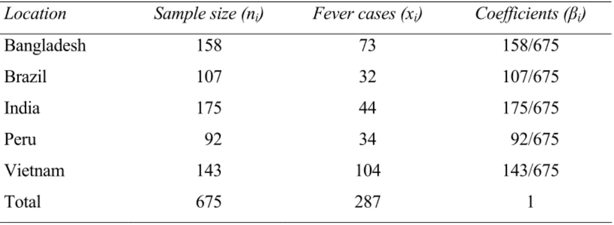
On other occasions, the linear combination L is not a contrast (i0); thus, it is normally interesting to determine a CI for L, which can also be obtained through inversion of the test for H: L=. This is the case with the multicenter clinical trials (Table 2) referred to by
Tebbs and Roth (2008) where the aim was to assess the efficiency of a reduced-salt diet in the treatment of male infants for acute watery diarrhea. One of the characteristics measured was the number of infants who had fever when admitted or during the trial. The aim is to estimate the pooled proportion of subjects who respond to treatment. Since the level of participation is likely to be different depending on the location, a natural estimate of the pooled proportion is the average of the response probabilities from the K=6 sites, i.e. L=βipi with βi=ni/nh
It has been observed that cited asymptotic inferences may refer to the application of a hypothesis test regarding L (H: L= vs. K: L, where is a constant so that
0 0
i i i i
) or to the determination of a CI for L. As the CI can be obtainedthrough inversion of the test and the test can be carried out through the CI, in practice the procedure used is the most comfortable one. Nonetheless, both types of inference will be explained.
Whatever the situation, the inferences about L can be carried out through diverse procedures. Price and Bonett (2004) and Schaarschmidt et al. (2008) improved the classic Wald method through the increase in data of a certain number of successes and failures (adjusted Wald methods). These procedures originate in similar proposals made by Agresti and Coull (1998) in the case of one proportion and by Agresti and Caffo (2000) in the case of the difference between two proportions. Martín et al. (2010) solved the problem through the score method, propose new adjusted Wald methods, justified that all of them are an approach to the score method and, finally, compared the methods obtained. These authors concluded that the score method was the best, closely followed by a modification and generalization of the method proposed by Price and Bonett. Finally, Newcombe (2001) for K=4 and i=0, and Zou et al. (2009) for any value of K and of i, suggest substituting the proportions of the Wald method with the boundaries of Wilson’s CI (1927).
This article has two objectives (both are limited to the relatively unstudied case of
K>2): proposing new methods and comparing them to the best methods proposed in the literature (with the aim of the selecting the best one). In general, we will consider that the best method is the one which gives CIs whose coverage is not normally excessively lower than the nominal one, while also having an average coverage which is close to the nominal one and a small average length (for more details see Section 3.1).
2. METHODS TO PERFORM INFERENCES. 2.1. Generalities regarding the basic test to be used.
Let K be independent binomial random variables xi~B(ni, pi) with i=1, 2,…, K, and let
L=ipi be the parameter of interest (with the proportions pi unknown and the parameters βi known). As the statistic L=Σipi, with pi=xi/ni, is asymptotically normal with a mean
L=ipi and variance i2piqi/ni, where qi=1–pi, then in order to test H: L= vs. K: L
(where 0 0
i i i i
2 2 2 exp i i i i L z p q / n
, (1) with 2 2 /z (where z/2 is the α/2-upper percentile of the typical normal distribution). The inversion of the test, i.e. making 2 2
2
exp /
z z and clearing λ, gives(1–α)-CI (L1; L2) for L. These expressions have no use until the unknown pi proportions are substituted with some of their estimations. From now on, let n=ni, B+=
0 i i
, B–= 0 i i
and B=βi.2.2. Estimation of the unknown proportions pi: the inference procedures involved.
The simplest and most well known option is to substitute pi with pi in expression (1). This leads to the following classic Wald statistics and Wald CI (where qi 1 pi):
2 2 W 2 i i i i L z p q n
, CIW: L± zα/2
i2p q ni i i , (2)thus we obtain what we will now call procedure W.
Another more complicated option is that proposed by Zou et al. (2009), who
theoretically justify and generalize the procedure proposed by Newcombe (1998, 2001) for certain special cases of K=2 and K=4. The procedure (which we will henceforth refer to as the N procedure) consists of substituting the unknown proportions pi with an appropriate limit pi
of the Wilson CI (1927) for the same ones:
(if 0), (if 0) when
(if 0), (if 0) when
i i i i i i i i i u l L p l u L , where 2 2 2 2 2 2 2 2 2 2 2 2 2 2 2 4 2 4 and / / i i / / i i i / i / i i i i i / i / z z x y z z x y x z x z n n l u n z n z ,
and therefore (the CI that follows is not the original expression of Zou et al.):
2 2 2 N 2 2 if if L R L< z L R L> ,
1 2 N 2 2 CI : / / L L z R L L z R , (3) where:
2 2 2 2 0 0 0 0 1 1 1 1 (+) ( ) i i i i i i i i i i i i i i i i i i i i u u l l l l u u R = , R = n n n n
.The two previous procedures are based on estimators of the proportions pi which are not restricted by the null hypothesis H: L=. Martín et al. (2010) proposes substituting the pi with the maximum likelihood estimators ˆpi under H, obtaining the CI through inversion of the test. This leads to the procedure S (since, as the aforementioned authors have demonstrated, the method is equivalent to the score method), and it consists of solving the equation:
y=n+(B–2λ)C–Ri=0 where C=zS2/(L–λ) (4)
with 2 2 2 2 2
i i i i i i
R n C n b C and bi=1–2 pi. When the objective is to carry out the test (in which case λ is known) and L≠λ, then 2
S
z is the only solution 2 S
z ≠0 for equation (4); when
L=λit is assumed that 2 S
z =0. When the objective is to obtain the CI L1<L<L2 (in which case
2 S z = 2
2
/
z is known), then Li are the only two solutions i for equation (4).
The argumentation which now follows -which is based on the criteria of Sterne (1954) and was used by Peskun (1993) in the case of the difference in proportions- gives the new procedure P based on a new estimation pi of the proportions pi subject to H (see the appendix). The score test for H: ipi= will be significant if zS2z2/2 in all of the pi values so that βipi=λ. Consequently, the objective should be to determine the minimum value of zS2, i.e. the maximum value of V= 2
i
piqi/ni, subject to the condition βipi=λ. In the appendix, it is demonstrated that the new statistic and the new CI are, respectively:
2 2 2 2 4 2 P i i L z B n n
,
2 2 2 2 2 2 2 P 2 2 2 CI : 2 2 / / / i / i B L n Bz z n z L n z n n n n
. (5)2.3. Original data and increased data.
Price and Bonett (2004), encouraged by the results of Agresti and Coull (1998) and Agresti and Caffo (2000) in the case of one proportion and the difference in proportions respectively, found that the Wald CI improves substantially if expression (2) is obtained based on the data xi+hi, yi+hi y ni+2hi, where hi=2/K, i.e. if we add to the original data 2/K successes and 2/K failures. This leads to the adjusted Wald method W1 in contrast to the original Wald method W0. More recently, Martín et al. (2010) found that best option for the adjusted Wald method is given by the method W3, which is obtained developing in a Maclaurin series expression (4), in which:
2 2 2 2 1 if 0 and 0 or 1 and 0 (1 ) if 0 otherwise 2 where (1 ) 1 if 0 and 0 or 1 and 0 if 2 0 otherwise i i i i / i i i / i i i i i i p p z I K I L K h z S K p p L S K , (6)although a good alternative is method W2 based on hi=z2/2 / K2 . It can be observed that when 0<xi<ni (i) then W2=W3, and if =5% is chosen then z2/2/ K2 2/K and W1W2=W3. When xi=0 or xi=ni in any value of i (i.e. when some observed data is found on the bound of the sample space), the calculations of method W3 become complicated since in this case the value of hi is different depending on if we are going to determine the lower bound L1 (when L ) or the upper bound L2 (whenL).
It can be observed that procedure W gives four methods (W0, W1, W2 and W3) based on the increases hi=0, 2/K, z2/2 / K2 and the one indicated in expression (6), respectively. The same can be done with the other three procedures (S, N and P), thus obtaining 16 methods W0,..., W3, S0,..., S3, N0,..., N3, P0,... and P3 which are going to be compared in this article.
3. SIMULATION STUDY. 3.1. Selection of the best methods.
The initial objective of this section is to compare the 16 methods proposed Wx, Zx, Sx, Px, where x=0, 1, 2 or 3. The comparison can be made from a double perspective: from the perspective of hypothesis tests or from the perspective of the CIs. As the evaluations are equivalent (if both are carried out to the same nominal error of α), in this section the comparison will be made from the perspective of the CIs (as they are the most habitual inferences in this context). In this sense, it is necessary to take into account the fact that in order to assess a CI, it is normal to use the parameters of real coverage and mean length, and to assess a test, it is normal to use the parameters of real error and power. As the real coverage and the real error add up to 1 and, moreover, the greater the power of the test the lower the length of the CI which is obtained through inversion, the consequence is that both evaluations are equivalent.
For the 100(1)% CI, the actual probability of coverage R and the expected interval length l for fixed pi values are defined by:
1 2 1 2 1 2 0 0 0 1 K i i i K n n n K i x n x i i K x x x i i n R ... p q I x ,x ,...,x x
and 1 2
1 0 2 0 0 1 K i i i K n n n K i x n x i i S I x x x i i n l ... p q L L x
where I(x1, x2, ..., xK)=1 if the CI (LI, LS) which causes the observations (x1, x2, ..., xK) contains
L=ipi and I(x1, x2, ..., xK)=0 in another case. For each set of values (ni, i) of Tables 3 (K=3 and =5%) and 4 (K=4 and =5%), 10,000 sets of pi´s were randomly generated from the uniform [0, 1] distribution, and those of the previous methods were used to compute l and R. The mean of
R (Rmean) and l (lmean) and the percentage of R that fell below 93% (R<93) in the 10,000 sets of pi´s were computed for 1=95%. The selection of the optimal method will be made based on the following rules (listed in order of importance): (i) the method must have few liberal “failures” (i.e. its R<93 value must be as small as possible); (ii) the method must have an Rmean
as near as possible to 95% (the method will be conservative if Rmean>95%, and liberal if
Rmean< 95%); (iii) the method must have an lmean which is as small as possible. These rules must not be applied in an excessively strict manner since, in an extreme case, it is of no use if the method gives an R<93 value equal to zero if its Rmean=100%.
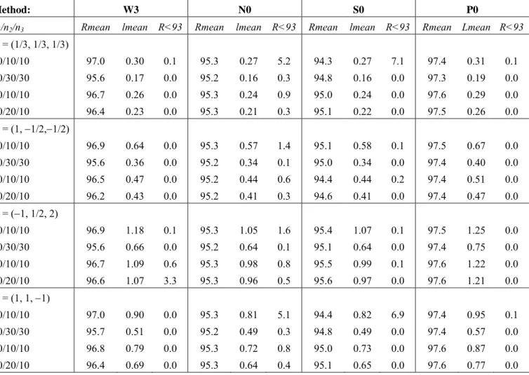
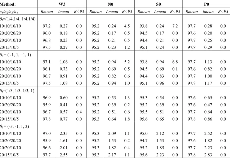
Tables 3 and 4 show the results for the best method of each family (the four methods W3, N0, S0 and P0) and for a confidence of 95%. The rest of the data can be requested from the authors. It is observed that:
(1) The N0 method has Rmean values which are very close to the nominal 95% (on average it is slightly conservative), but it fails a great deal and in all circumstances (since its R<93
values are usually too large) and, therefore, it must be rejected.
(2) The P0 and W3 methods are both very conservative (the Rmean values are much greater than 95%) and very imprecise (high lmean values), although the W3 method is less extreme in these two aspects. Both methods fail very little (their R<93 value is small), although the P0 method fails somewhat less. Therefore, in overall terms, the W3 method is preferable to the P0 method.
(3) The S0 method has the best Rmean values (they are the most balanced around 95%) and
lmean values (they are the smaller than those of the P0 and W3 methods) and only fails too much on some occasions in which ni=10 (i), and thus it can be deduced that it is the best method when the samples are not excessively small.
Therefore, it is deduced that S0 is the best method, although if the samples are very small (ni 10, i) the W3 method is the best. It is also observed that the W3 method is a much simpler alternative to the S0 method, although it is somewhat conservative, with some mistakes and it leads to wider CIs than those of the S0 method. Finally, the P0 method would be the optimal method if we require a method that almost never fails, although this implies using a method that is too conservative and that leads to excessively wide CIs. These conclusions also hold in
general for confidences of 90% and 99% (the data can be requested from the authors), although the W3 and P0 methods are now very similar when K=4. It can also be observed that the same conclusions hold in the case of a contrast (i=0), and the only difference is that now the W3 method practically never fails.
3.2. Continuity correction methods.
The second objective of this article is to check whether continuity correction (‘cc’ from now on) manages to improve the performance of the methods selected in the previous section (W3, S0 and P0). It is well known (Cox, 1970) that it is useful to make a cc when the distribution of a discrete random variable (such as the variable xi) is approximated through a continuous variable (such as the normal variable). Haber (1980) proposed that a cc should consist of adding to or subtracting from the variable half of its average jump. In our case, the variable is L (the contrast statistic) and, as B L B (since 0
i
p 1), its total jump will be
i and half of its average jump, i.e. the cc, will be c
i
/ 2
N1
, with
i 1
N n , since N is the total number of points (x1, ... , xK) of the sample space. In the case of one proportion, the classic cc c=1/2n is obtained. In the case of the difference between two proportions, c=1/(n1n2+n) is obtained, which is the cc of Martín and Herranz (2004).
In order to determine the 2
exp
z statistic of expression (1) with cc it is sufficient to redefine it in the following way: 2
c
z =0 if L c and 2 2
2
2c exp
z z L c / L if
L c. This gives rise to the new statistics 2
Wc
z , 2
Nc
z and 2
Pc
z obtained through expressions (2), (3) and (5), respectively. In the case of the score test, the statistic 2
Sc
z is obtained changing the 2
S
z value of expression (4) for the value 2
2Sc
z L / L c , when 2
Sc
z is the unknown quantity of said equation. In a similar way, in order to determine the CI of expression (1) with cc, it is sufficient to add to it the term ±c. This gives rise to the new intervals CIWc, CINc and CIPc obtained through expressions (2), (3) and (5) respectively. In the case of the CISc of the scores, it is sufficient to change the zS2 value of expression (4) for
22 2
/
z L / L c and to determine its two i solutions with B1 L c and 2
L c B. Whatever the case (CI or test), the introduction of the cc leads to four new procedures Wc, Nc, Sc y Pcand 16 new methods Wxc, Nxc, Sxc and Pxc, withx=0, 1, 2 y 3.
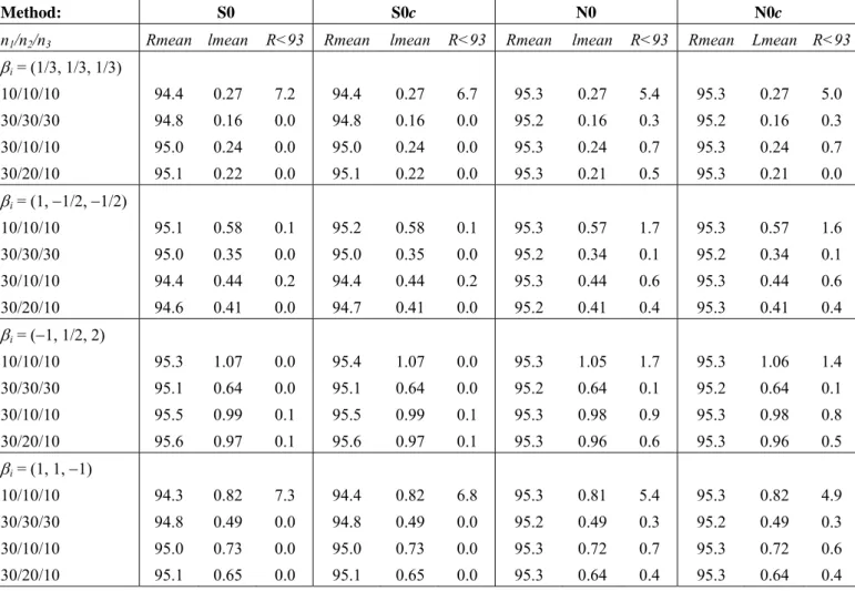
It is clear that cc is not useful in the case of the W and P procedures since, as the cc causes the p-value to decrease, the Wc and Pc procedures will be even more conservative and more imprecise than the originals. Therefore, Table 5 (for K=3 and =5%) only considers the
N0, N0c, S0 and S0c methods. It must be taken into consideration that, in the interests of comparability, this new table has been obtained for a different sequence of 10,000 sets of pi´s; therefore, the data for S0 and N0 are not exactly the same as in Tables 3 and 5. Observing Table 5 it is deduced that:
(1) As was to be expected, in all cases the S0c and N0c methods have a lower or equal number of failures than those of the S0 and N0 methods respectively.
(2) The S0 and S0c methods are the same in all of the parameters, except when ni=10 (i) in which S0c is somewhat better than S0 as it has fewer failures. Nevertheless, in this last case, S0c is still not competitive in relation to the W3 method selected in the previous evaluation.
(3) The N0c method is slightly better than the N0 method in regard to the number of failures, although this is in exchange that N0 is slightly better than N0c in terms of Rmean and
lmean. As this does not imply that N0 improves its performance in order to be competitive with the optimal methods S0c and W3, it is deduced that the cc has no interest in this case. Thus, it can be observed that, when K=3, cc is only useful to slightly improve the S method when the samples are small. As the cc decreases sharply with K, it is deduced that its interest will be even greater in the case of K>3.
3.3. Final selection.
From the aforementioned information, it is deduced that: (1) if ni 10 (i), W3 is the best method; (2) in another case, S0 is the best, but a much simpler alternative is method W3 (although is rather conservative, has some failures and causes CIs which are broader than S0); (3) if we need a method which never fails, we can choose the method P0 (but it is too conservative and gives excessively broad CIs); (4) if we need to use the same method, the best option is method S0c.
4. EXAMPLES.
For the data in Table 1, the Sc method applied to the contrasts L1, L2 and L3 provides the values zSc = 0.412, 2.424 and +2.803, respectively, which indicates that the effects of fiber and fat are significant but there is no interaction between them. In order to quantify the
magnitude of the effects of L2 and L3, it is necessary to determine the CI for each one of them. Alternatively, the aforementioned tests can be carried out through the CI for L1, L2 and L3 (as in the next paragraph).
Table 6 contains the 95%-CIs for all of the contrasts in Table 1 and the combination of that of Table 2 made by the methods selected in the previous section (S0c, W3 and P0) and through the N0 method. It can be observed that all of the methods indicate that the contrasts
L2 and L3 are significant to an error of 5% (since its CIs do not contain the value 0), but that the contrast L1 is not (since its CIs contain the value 0). Nevertheless, in the evaluation of the magnitude of the different values of L there are some differences between the methods. It is observed that the N0 method gives narrower CIs than those of the other methods, although the advantage is only apparent: the simulation study indicated that the N0 method had many failures (it is excessively liberal on too many occasions). It is also observed that the P0 method provides excessively wide CIs, except when the sample sizes are large (as in the case of L). Finally, it is observed that the W3 method provides CIs of a similar width to that of the S0c method, although its centers are rather different (except in the case of L, once again due to the high values of ni).
5. CONCLUSIONS.
Asymptotic inferences (tests or CIs) about a linear combination (L=ipi) of K independent binomial proportions pi are very frequent in applied research (Tebbs and Roths, 2008). Historically, literature in this field has paid special attention to the case of K2 (which contains the cases with one proportion and the difference or ratio for two proportions), but there is increasing interest in the case of K>2 (Newcombe, 2001; Price and Bonett, 2004; Schaarschmidt et al. 2008; Tebbs and Roths, 2008; Agresti et al., 2008; Zou et al., 2009 and Martín et al., 2010). The linear combination L may be a contrast (i=0), in which case it is usually interesting to carry out the test for H: L=0 or to determine a confidence interval for L, or may not be (i0), in which case it is usually interesting to determine a CI for L; therefore this article has concentrated on the diverse procedures to carry out the test H: L= vs.K: L or to obtain a CI for L through inversion of the previous test.
In order to make the previous inferences, there are various procedures that have not been compared with each other: the S0 score method and the W3 Wald adjusted method defined by Martín et al. (2010) on the one hand, and the N0 method defined by Zou et al.
(1993), which is given by expressions (5). Additionally, the article modifies the previous methods giving them cc (the S0c, W3c, N0c and P0c methods, respectively) and demonstrates that the previous methods, which are different to those based on the Wald statistic, do not improve because of increasing the successes and failures in determined quantities. Finally, in the article, a simulation experiment is performed to compare the eight cited procedures (S0, W3, N0, P0, S0c, W3c, N0c and P0c) and it is concluded that S0c is the best method, although for very small samples (ni 10, i), the W3 method is the best. The P0 method would be the best if we need a method that almost never fails, but is also an excessively conservative method and provides CIs that are too wide. The W3 and P0 methods have the
additional advantage of being very easy to apply. The optimal S0c method has the
disadvantage of requiring an iterative process; at http://www.ugr.es/local/bioest/Z_LINEAR_ K.EXE a free programme can be obtained for the S0 and S0c methods.
6. ACKNOWLEDGEMENTS.
This research was supported by the Spanish Ministry of Education and Science, grant number MTM2009-08886 (co-financed by the European Regional Development Fund) and by the Department of Innovation, Science and Business of the Autonomous Government of Andalusia, Spain, grant number FQM-01459.
APPENDIX: Obtaining the Sterne-Peskun procedure
For what follows the following inequalities will be useful (where B=i):
–|βi| ≤B–2λ, B–2L ≤ +|βi| (A1) which are because
0 0 i i B , L B i i
since λ=βipi, L=βipi and 0≤ pi,pi≤+1.As was indicated in Section 2.2, the objective is to determine the maximum value of
V= 2
i
piqi/ni subject to the condition λ=βipi. The condition implies that dpK/dpi=–βi/βK (i≠K), so that Vi= dV/dpi = (∂V/∂pi)–(βi/βK)(∂V/∂pK) = βi{βi(1–2pi)/ni–βK(1–2pK)/nK}=0 (iK) when βi(1–2pi)/ni=γ (i), with γ a constant that has yet to be determined. As niγ= βi– 2βipi, then adding in i it holds that nγ=B–2λ, where |B–2λ|≤|βi| through expression (A1). Therefore, V reaches a bound in:
0 1 1 where 2 and 2 i i i i i | | n B p p | | n n
(A2)This bound is a maximum since d2V/d 2
i
p =(∂V′/∂pi)–(βi/βK)(∂V′/∂pK) = –2i2(1/ni+1/nK)<0, and its value will be V0= i2pi0qi0/ni= {i2/ni–nγ
2}/4, with q
i0=1–pi0. This leads to the first expression (5).
In order for V0 to be a valid value it is necessary for V0≥0. In order to see this, let
f=4V0=i2/ni–nγ2. As df/dβi = 2βi/ni–2γ = 0 when βi/ni=γ and as d2f /di2=2(nni)/nni>0, then f reaches a minimum when βi=niγ (i) and therefore f ≥minif= 0.
In order for the inference to be coherent, it is necessary for the statistic 2
P
z to be decreasing (increasing) in λ when λ<L (λ>L) so that the p-value is increasing (decreasing) in
λ. As d 2
P
z /dλ = –(L–λ)g/(2 2 0
V ), with g = 4V0+2(L–λ)γ = i2/ni–(B–2L)(B–2λ)/n, the condition demanded will be verified if g≥0. When (B–2L) and (B–2λ) has different signs,
g≥0 without doubt. In another case, g = 2
i
/ni–|B–2L||B–2λ|/n ≥ i2/ni–(|βi|)2/n = h for expression (A1). Deriving h in |βi| it is observed that h reaches a minimum when |βi| =
ni(|βi|)/n (i). As this minimum is 0, then h≥0.
Expression (5) is based on the pi0 values of expression (A1), values that will be legitimate if 0≤ pi0≤1, i.e. if |γ| ≤ |βi|/ni or, equivalently if:
1 2 i i | | B n (A3)
When pi0<0 o pi0>1, it seems appropriate to substitute them for pi0=0 or pi0=1, respectively. If this is done so, pi0qi0=0 and those terms do not contribute to the V0 value. This provides the new statistic (which is just as simple as the previous one):
2 2 2 0 0 1 where and 4 i i i P I i I i L | | z V n I i | | V n n
(A4) Making 2 2 2 / Pz z and clearing λ, the (1–α)-CI is obtained for L: 2 2 2 2 2 2 2 2 2 2 2 2 P 2 2 CI : 2 2 / / / / n nz B z n nz B L L S n n nz n n n (A5) with i I n
n and 2 i i IS
/ n . It should be observed that expression (A5) contains the first expression (5). The problem with this new CI is that its determination may require theapplication of expression (A5) several times. In order to obtain the previous CI , it is P necessary to carry out the following steps: (i) Make I={1, 2, …, K} and obtain the two λI and
λS values which provide expression (A5); (ii) If λI and λS verify expression (A3) iI, the process finishes; (iii) In another case, the bound that has failed must be obtained again for a new I set which is obtained eliminating from the previous one all of the r values so that |βr|/nr = MiniI |βi|/ni; (iv) This must be done successively until the process finishes, i.e. until λI and
λS verify expression (A3) all of the iI values, when I is the set associated with the λI or λS value considered. In this article, the current P procedure is discarded since, as it is more complicated than the P procedure, it does not improve the results (data can be requested from the authors).
References
Agresti, A. (2003). Dealing with discreteness: making ‘exact’ confidence intervals for proportions, differences of proportions, and odds ratios more exact. Statistical Methods in Medical Research12, 3-21. DOI:10.1191/0962280203sm311ra.
Agresti, A. and Caffo, B. (2000). Simple and effective confidence intervals for proportions and difference of proportions result from adding two successes and two failures. The American Statistician 54 (4), 280-288.
Agresti, A. and Coull, B. A. (1998). Approximate Is Better than "Exact" for Interval Estimation of Binomial Proportions. The American Statistician 52 (2), 119-126.
Agresti, A.; Bini, M.; Bertaccini, B. and Ryu, E. (2008). Simultaneous confidence intervals for comparing binomial parameters. Biometrics 64, 1270-1275. DOI: 10.1111/j.1541-0420.2008.00990.x.
Cohen, L. A.; Kendall, M. E.; Zang, E.; Meschter, C. and D. P. Rose (1991). Modulation of N-Nitrosomethylurea-Induced Mammary Tumor Promotion by Dietary Fiber and Fat.
Journal of National Cancer Institution 83, 496-501. DOI: 10.1093/jnci/83.7.496.
Cox, D.R. (1970). The continuity correction. Biometrika 57, 217-219. DOI: 10.1093/biomet/ 57.1.217.
Haber, M. (1980). A comparison of some continuity corrections for the chi-squared test on 22 tables. Journal of the American Statistical Association 75, 510-515.
Martín Andrés, A., Álvarez Hernández, M. and Herranz Tejedor, I. (2010). Inferences about a linear combination of proportions. Statistical Methods in Medical Research. Prepublihed March 11, 2010, DOI: 10.1177/0962280209347953.
Martín Andrés, A. and Herranz Tejedor, I. (2004). Asymptotical tests on the equivalence, substantial difference and non-inferiority problems with two proportions. Biometrical Journal 46 (3), 305-319. DOI: 10.1002/bimj.200310041.
Newcombe, R.G. (1998). Interval estimation for the difference between independent proportions:
comparison of eleven methods. Statistics in Medicine 17, 873-890. DOI:
10.1002/(SICI)1097-0258(19980430).
Newcombe, R.G. (2001). Estimating the difference between differences: measurement of additive scale interaction for proportions. Statistics in Medicine 20 (19), 2801-2994. DOI: 10.1002/sim.925.
Peskun, P.H. (1993). A new confidence interval method based on the normal approximation for the difference of two binomial probabilities. Journal of theAmerican Statistical Association 88 (422), 656-661.
Pham-Gia, T. and Turkkan, N. (1994). Reliability of a standby system with beta-distributed component lives. IEEE Transactions on Reliability 43(1), 71-75.
Phillips, K.F. (2003). A new test of non-inferiority for anti-infective trials. Statistics in Medicine 22, 201-212. DOI: 10.1002/sim.1122.
Price, R. M. and Bonett, D. G. (2004). An improved confidence interval for a linear function of binomial proportions. Computational Statistics & Data Análisis 45 (3), 449-456. DOI :
10.1016/S0167-9473(03)00007-0.
Schaarschmidt, F.; Sill, M. and Hothorn, L.A. (2008). Approximate Simultaneous Confidence Intervals for Multiple Contrasts of Binomial Proportions. Biometrical Journal, 50 (5), 782-792. DOI: 10.1002/bimj.200710465.
Sterne, T.E. (1954). Some remarks on confidence of fiducial limits. Biometrika 41 (1/2), 275-278.
Tebbs, J. M. and Roths, S. A. (2008). New large-sample confidence intervals for a linear combination of binomial proportions. Journal of Statistical Planning and Inference 138 (6), 1884-1893. DOI: 10.1016/j.jspi.2007.07.008.
Wilson, E.B. (1927). Probable inference, the law of succession, and statistical inference. Journal of the American Statistical Association 22, 209-212.
Zou, G.; Huang, W. and Zhang, X. (2009). A note on confidence interval estimation for a linear function of binomial proportions. Computational Statistics & Data Analysis 53, 1080-1085. DOI: 10.1016/j.csda.2008.09.033.
Table 1: Diet and tumor study
Fiber No Fiber
High Fat Low Fat High Fat Low Fat
Sample size (ni) 30 30 30 30
Rats showing cancer (xi) 20 14 27 19
Effect Β1 Β2 β3 β4
L1=Fiber×Fat +1 –1 –1 +1
L2=Fiber +1 +1 –1 –1
L3=Fat +1 –1 +1 –1
Table 2: Multicenter clinical trial data
Location Sample size (ni) Fever cases (xi) Coefficients (βi) Bangladesh Brazil India Peru Vietnam Total 158 107 175 092 143 675 73 32 44 34 104 287 158/675 107/675 175/675 092/675 143/675 1
Table 3: Mean coverage values (Rmean), mean length values (lmean) and percentage of coverages which are lower than 93% (R<93) for 95%-CI obtained through the W3, N0, S0 and P0 methods (K=3).
Method: W3 N0 S0 P0
n1/n2/n3 Rmean lmean R<93 Rmean lmean R<93 Rmean lmean R<93 Rmean Lmean R<93
i = (1/3, 1/3, 1/3) 10/10/10 30/30/30 30/10/10 30/20/10 97.0 95.6 96.7 96.4 0.30 0.17 0.26 0.23 0.1 0.0 0.0 0.0 95.3 95.2 95.3 95.3 0.27 0.16 0.24 0.21 5.2 0.3 0.9 0.3 94.3 94.8 95.0 95.1 0.27 0.16 0.24 0.22 7.1 0.0 0.0 0.0 97.4 97.3 97.6 97.5 0.31 0.19 0.29 0.26 0.1 0.0 0.0 0.0 i = (1, 1/2,1/2) 10/10/10 30/30/30 30/10/10 30/20/10 96.9 95.6 96.5 96.2 0.64 0.36 0.47 0.43 0.0 0.0 0.0 0.0 95.3 95.2 95.2 95.2 0.57 0.34 0.44 0.41 1.4 0.1 0.6 0.3 95.1 95.0 94.4 94.6 0.58 0.34 0.44 0.41 0.1 0.0 0.2 0.0 97.5 97.4 97.4 97.4 0.67 0.40 0.51 0.47 0.0 0.0 0.0 0.0 i = (1, 1/2, 2) 10/10/10 30/30/30 30/10/10 30/20/10 96.9 95.6 96.7 96.6 1.18 0.66 1.09 1.07 0.1 0.0 0.6 3.3 95.3 95.2 95.3 95.3 1.05 0.64 0.98 0.96 1.6 0.1 0.8 0.5 95.4 95.1 95.5 95.6 1.07 0.64 0.99 0.97 0.1 0.0 0.1 0.0 97.5 97.4 97.6 97.6 1.25 0.75 1.22 1.21 0.0 0.0 0.0 0.0 i = (1, 1, 1) 10/10/10 30/30/30 30/10/10 30/20/10 97.0 95.7 96.8 96.4 0.90 0.51 0.79 0.69 0.0 0.0 0.0 0.0 95.3 95.2 95.3 95.3 0.81 0.49 0.72 0.64 5.1 0.3 0.8 0.4 94.4 94.8 95.0 95.1 0.82 0.49 0.73 0.65 6.9 0.0 0.0 0.0 97.4 97.4 97.6 97.6 0.95 0.57 0.87 0.77 0.1 0.0 0.0 0.0
Table 4: Mean coverage values (Rmean), mean length values (lmean) and percentage of coverages which are lower than 93% (R<93) for 95%-CI obtained through the W3, N0, S0 and P0 methods (K=4).
Method: W3 N0 S0 P0
n1/n2/n3/n4 Rmean lmean R<93 Rmean Lmean R<93 Rmean Lmean R<93 Rmean lmean R<93
I=(1/4,1/4, 1/4,1/4) 10/10/10/10 20/20/20/20 20/20/10/10 20/15/10/5 97.2 96.0 96.8 97.5 0.27 0.18 0.23 0.27 0.0 0.0 0.0 0.0 95.2 95.2 95.2 95.2 0.24 0.17 0.21 0.23 4.5 0.5 0.5 1.2 93.8 94.5 94.4 95.1 0.24 0.17 0.21 0.24 7.2 0.0 0.0 0.0 97.7 97.6 97.7 97.8 0.28 0.20 0.25 0.29 0.0 0.0 0.0 0.0 i = ( -1, 1, 1, 1) 10/10/10/10 20/20/20/20 20/20/10/10 20/15/10/5 97.1 96.1 96.7 97.5 1.06 0.73 0.91 1.08 0.0 0.0 0.0 0.0 95.2 95.2 95.2 95.2 0.94 0.69 0.82 0.94 5.2 0.5 0.6 1.0 93.8 94.5 94.4 95.1 0.94 0.69 0.83 0.96 6.8 0.1 0.0 0.0 97.7 97.6 97.7 97.8 1.13 0.82 1.00 1.17 0.0 0.0 0.0 0.0 I=(1/3, 1/3, 1/3, 1) 10/10/10/10 20/20/20/20 20/20/10/10 20/15/10/5 96.9 95.9 96.7 97.8 0.60 0.41 0.57 0.77 0.0 0.0 0.4 0.0 95.2 95.2 95.2 95.3 0.53 0.39 0.51 0.64 1.3 0.2 0.6 1.8 95.3 95.2 95.5 95.6 0.54 0.39 0.51 0.65 0.0 0.0 0.0 0.0 97.6 97.6 97.7 97.8 0.65 0.47 0.64 0.86 0.0 0.0 0.0 0.0 i = (-3, -1, 1, 3) 10/10/10/10 20/20/20/20 20/20/10/10 20/15/10/5 97.0 95.9 96.6 97.7 2.35 1.61 2.01 2.55 0.0 0.0 0.0 0.0 95.3 95.2 95.3 95.3 2.09 1.53 1.82 2.17 1.1 0.2 0.4 1.1 95.0 94.7 95.2 95.6 2.12 1.53 1.85 2.23 0.0 0.0 0.0 0.0 97.7 97.6 97.7 97.8 2.52 1.82 2.23 2.83 0.0 0.0 0.0 0.0
Table 5: Mean coverage values (Rmean), mean length values (lmean) and percentage of coverages which are lower than 93% (R<93) for 95%-CI obtained through the S0, S0c, N0 and N0c methods (K=3). Method: S0 S0c N0 N0c
n1/n2/n3 Rmean lmean R<93 Rmean lmean R<93 Rmean lmean R<93 Rmean Lmean R<93
i = (1/3, 1/3, 1/3) 10/10/10 30/30/30 30/10/10 30/20/10 94.4 94.8 95.0 95.1 0.27 0.16 0.24 0.22 7.2 0.0 0.0 0.0 94.4 94.8 95.0 95.1 0.27 0.16 0.24 0.22 6.7 0.0 0.0 0.0 95.3 95.2 95.3 95.3 0.27 0.16 0.24 0.21 5.4 0.3 0.7 0.5 95.3 95.2 95.3 95.3 0.27 0.16 0.24 0.21 5.0 0.3 0.7 0.0 i = (1, 1/2, 1/2) 10/10/10 30/30/30 30/10/10 30/20/10 95.1 95.0 94.4 94.6 0.58 0.35 0.44 0.41 0.1 0.0 0.2 0.0 95.2 95.0 94.4 94.7 0.58 0.35 0.44 0.41 0.1 0.0 0.2 0.0 95.3 95.2 95.3 95.2 0.57 0.34 0.44 0.41 1.7 0.1 0.6 0.4 95.3 95.2 95.3 95.3 0.57 0.34 0.44 0.41 1.6 0.1 0.6 0.4 i = (1, 1/2, 2) 10/10/10 30/30/30 30/10/10 30/20/10 95.3 95.1 95.5 95.6 1.07 0.64 0.99 0.97 0.0 0.0 0.1 0.1 95.4 95.1 95.5 95.6 1.07 0.64 0.99 0.97 0.0 0.0 0.1 0.1 95.3 95.2 95.3 95.3 1.05 0.64 0.98 0.96 1.7 0.1 0.9 0.6 95.3 95.2 95.3 95.3 1.06 0.64 0.98 0.96 1.4 0.1 0.8 0.5 i = (1, 1, 1) 10/10/10 30/30/30 30/10/10 30/20/10 94.3 94.8 95.0 95.1 0.82 0.49 0.73 0.65 7.3 0.0 0.0 0.0 94.4 94.8 95.0 95.1 0.82 0.49 0.73 0.65 6.8 0.0 0.0 0.0 95.3 95.2 95.3 95.3 0.81 0.49 0.72 0.64 5.4 0.3 0.7 0.4 95.3 95.2 95.3 95.3 0.82 0.49 0.72 0.64 4.9 0.3 0.6 0.4
Table 6: Analysis of the data in Tables 1 and 2
CI (Tables 1 and 2) = center (first entry) ± radius (second entry)
Method L1 L2 L3 L
S0c .0719 .3164 .3934 .3162 .4581 .3161 .4256 .0349
W3 .0646 .3162 .3876 .3162 .4522 .3162 .4256 .0348
N0 –.0702 .3088 –.3834.3084 .4465 .3082 .4261 .0345